Interactive Markov Models of Evolutionary Algorithms

Cleveland State University

EngagedScholarship@CSU

Electrical Engineering & Computer Science Faculty

Publications

Electrical Engineering & Computer Science

Department

2015

Interactive Markov Models of Evolutionary

Algorithms

Haiping Ma

Shanghai University

Daniel J. Simon

Cleveland State University, [email protected]

Minrui Fei

Shanghai University

Hongwei Mo

Harbin Engineering University

Follow this and additional works at:

https://engagedscholarship.csuohio.edu/enece_facpub

Part of the

Electrical and Computer Engineering Commons

How does access to this work benefit you? Let us know!

Publisher's Statement

(c) 2016 IEEE. Personal use is permitted, but republication/redistribution requires IEEE

permission. See http://www.ieee.org/publications_standards/publications/rights/index.html for

more information. This article has been accepted for publication in a future issue of this journal, but

has not been fully edited. Content may change prior to final publication.

Repository Citation

Ma, Haiping; Simon, Daniel J.; Fei, Minrui; and Mo, Hongwei, "Interactive Markov Models of Evolutionary Algorithms" (2015).Electrical Engineering & Computer Science Faculty Publications. 390.

https://engagedscholarship.csuohio.edu/enece_facpub/390

This Article is brought to you for free and open access by the Electrical Engineering & Computer Science Department at EngagedScholarship@CSU. It has been accepted for inclusion in Electrical Engineering & Computer Science Faculty Publications by an authorized administrator of

EngagedScholarship@CSU. For more information, please [email protected].

Original Citation

H. Ma, D. Simon, M. Fei and H. Mo, "Interactive Markov Models of Optimization Search Strategies," IEEE Transactions on Systems, Man, and Cybernetics: Systems, vol. PP, pp. 1-18, 2015.

Interactive Markov Models of Optimization

Search Strategies

Haiping Ma, Dan Simon, Senior Member, IEEE, Minrui Fei, and Hongwei Mo

Abstract—This paper introduces a Markov model for

evolu-tionary algorithms (EAs) that is based on interactions among individuals in the population. This interactive Markov model has the potential to provide tractable models for optimization prob-lems of realistic size. We propose two simple discrete optimization search strategies with population-proportion-based selection and a modified mutation operator. The probability of selection is lin-early proportional to the number of individuals at each point of the search space. The mutation operator randomly modifies an entire individual rather than a single decision variable. We exactly model these optimization search strategies with interac-tive Markov models. We present simulation results to confirm the interactive Markov model theory. We show that genetic algo-rithms and biogeography-based optimization perform better with the addition of population-proportion-based selection on a set of real-world benchmarks. We note that many other EAs, both new and old, might be able to be improved with this addition, or modeled with this method.

Index Terms—Evolutionary algorithm (EA), interactive Markov model, Markov model, optimization search strategy, population-proportion-based selection.

I. INTRODUCTION

E

VOLUTIONARY algorithms (EAs) and swarm intelli-gence (SI) algorithms have received much attention over the past few decades due to their ability as global optimization search methods for real-world applications [1]–[3]. Some pop-ular EAs include the genetic algorithm (GA) [4], [5], evolu-tionary programming [6], differential evolution (DE) [7]–[10], Manuscript received June 23, 2015; accepted September 1, 2015. This work was supported in part by the National Science Foundation (NSF) under Grant 1344954, in part by the National Natural Science Foundation of China under Grant 61305078 and Grant 61533010, and in part by the Shaoxing City Public Technology Applied Research Project under Grant 2013B70004. The work of D. Simon was supported in part by the NASA Glenn Research Center, in part by the Cleveland Clinic, in part by the NSF, and in part by the several industrial organizations. The work of H. Ma and M. Fei was supported in part by the NSF, and in part by several industrial organizations. This paper was recommended by Associate Editor M. K. Tiwari.

H. Ma was with the Department of Electrical Engineering, Shaoxing University, Shaoxing 312000, China. He is now with the Shanghai Key Laboratory of Power Station Automation Technology, School of Mechatronic Engineering and Automation, Shanghai University, Shanghai 200072, China (e-mail:[email protected]).

D. Simon is with the Department of Electrical Engineering and Computer Science, Cleveland State University, Cleveland, OH 44115 USA (e-mail: [email protected]).

M. Fei is with the Shanghai Key Laboratory of Power Station Automation Technology, School of Mechatronic Engineering and Automation, Shanghai University, Shanghai 200072, China (e-mail:[email protected]).

H. Mo is with the Department of Automation, Harbin Engineering University, Harbin 150001, China (e-mail:[email protected]).

Digital Object Identifier 10.1109/TSMC.2015.2507588

evolution strategy (ES) [11], biogeography-based opti-mization (BBO) [12], [13]. SI algorithms include ant colony optimization (ACO) and particle swarm optimiza-tion (PSO) [14]–[16]. Inspired by natural processes, EAs and SI are search methods that are fundamentally different than traditional, analytic optimization techniques. EAs are based on the collective learning process of a population of candi-date solutions to an optimization problem. In this paper, we often use the shorthand term individual to refer to a candidate solution.

The population in an EA is usually randomly initialized, and each iteration (also called a generation) evolves toward better and better solutions by selection processes (which can be either random or deterministic), mutation, and recombi-nation (which is omitted in some EAs). The environment delivers quality information about individuals (fitness values for maximization problems, and cost values for minimization problems). Individuals with high fitness are selected to repro-duce more often than those with lower fitness. All individuals have a small mutation probability to allow the introduction of new information into the population.

Each EA and SI algorithm works on principles of different natural phenomena. For example, the GA is based on survival of the fittest, DE is based on vector differences of candi-date solutions, ES uses self-adaptive mutation rates, PSO is based on the flocking behavior of birds, ACO is based on the behavior of ants seeking food, and BBO is based on migration behavior. EAs all have certain features in common and proba-bilistically share information between candidate solutions to improve solution fitness. EAs have been applied to many optimization problems and have proven effective for solving various kinds of problems, including unimodal, multimodal, deceptive, constrained, dynamic, noisy, and multiobjective problems [17].

A. Evolutionary Algorithm Models

Although EAs have shown good performance on various problems, it is still a challenge to understand the kinds of problems for which each EA is most effective, and why. The performance of EAs depends on the problem representation and the tuning parameters. For many problems, when a good representation is chosen and the tuning parameters are set to appropriate values, EAs can be very effective. When poor choices are made for the problem representation or the tun-ing parameters, an EA might perform no better than random search. If a mathematical model could predict the improvement

in fitness from one generation to the next, it could be used to find optimal values of the problem representation or the tuning parameters.

For example, consider a problem with very expensive fitness function evaluations. For some problems we may even need to perform long, tedious, expensive physical experiments to eval-uate fitness. If we can find a model that reduces the number of required fitness function evaluations in an EA, we can use the model during the early generations to adjust the EA tun-ing parameters, or to find out which EAs will perform the best. A mathematical model of the EA could be useful to develop effective algorithmic modifications. More generally, an EA model could be useful to produce insights to how the algorithm behaves, and under what conditions it is likely to be effective.

There has been significant research in obtaining mathe-matical models of EAs. One of the earliest approaches was schema theory, which analyzes the growth and decay over time of various bit combinations in discrete EAs [4]. It has several disadvantages, including the fact that it is only approx-imate. Perhaps the most widely developed EA model is based on Markov theory [18]–[20], which has been a valuable theo-retical tool that has been applied to several EAs, including GAs [21] and simulated annealing [22]. Infinite population size Markov models are discussed in detail in [23], and exact finite population size Markov models are discussed in [24].

In Markov models, a Markov state represents an EA popu-lation distribution. Each state describes how many individuals there are at each point of the search space. The Markov model reveals the probability of arriving at any population given any starting population, in the limit as the genera-tion count approaches infinity. But the size of Markov model increases drastically with the population size and search space cardinality. These computational requirements restrict the application of the Markov model to very small problems, as we discuss in more detail in Section II.

B. Overview of the Paper

The first goal of this paper is to present a Markov model of EAs which is based on interactions among individuals. The standard EA Markov model applies to the population as a whole; that is, it does not explicitly model interac-tions among individuals. This approach is extremely limiting and leads to intractable Markov model sizes, as we show in Section II. In interactive Markov models we define the states as the possible values of each individual. This gives a separate Markov model for each individual in the population, but the separate models interact with each other. The transition prob-abilities for each Markov model are functions of the states of other Markov models, which is a natural and powerful exten-sion of the standard Markov model. This method can lead to a better understanding of EA behavior on problems with more realistic sizes.

The standard Markov model has a state space whose dimension grows factorially with search space cardinality and population size, while the interactive Markov model presented here has a state space whose dimension is independent of

population size and grows linearly with the cardinality of the search space. The interactive Markov model presented here is limited to EAs with a discrete search space and is still limited to relatively small problems, but is not nearly as limited as the standard Markov model, as we will see in Section II.

The second goal of this paper is to propose two sim-ple optimization strategies that use population-based selection probabilities. We call these strategies “population-proportion-based EAs.” We use a modified mutation operator in the EAs. The modified mutation operator randomly modifies (replaces) an entire individual rather than modifying a single decision variable. We exactly model these EAs with interactive Markov models. We confirm the interactive Markov model with simu-lation on a set of test problems. We then empirically compare standard GA and BBO with population-proportion-based GA and BBO on a set of real-world benchmarks to show the performance improvement that is possible.

Section II introduces the preliminary foundations of inter-active Markov models, presents two simple EAs, models them using an interactive Markov model, uses interactive Markov model theory to analyze their convergence, and discusses their computational complexity. Section III discusses the similari-ties and differences between our two simple EAs and standard, well-established EAs, including GA and BBO. Section IV explores the performance of the proposed optimization search strategies using both Markov theory and simulations, and shows that the inclusion of population-proportion-based selec-tion significantly improves both GA and BBO performance on real-world benchmarks. Section V presents some concluding remarks and recommends some directions for future work.

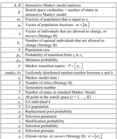
Notation: The symbols and notations used in this paper are

summarized in TableI.

II. INTERACTIVEMARKOVMODELS

Section II-A presents the foundation for interactive Markov models. Section II-B presents two proportion-selection-based EAs, and Section II-C discusses their convergence properties. Section II-D analyzes the interactive Markov model transi-tion matrix of the two EAs, and Sectransi-tion II-E discusses their computational complexities.

A. Fundamentals of Interactive Markov Models

A standard, noninteractive Markov model is a random pro-cess with a discrete set of possible states si(i = 1, . . . ,K),

where K is the number of possible states, also called the car-dinality of the state space. The probability that the system transitions from sj to si is given by the transition probabil-ity pij. The K×K matrix P=[pij] is the transition matrix. In standard noninteractive Markov models of EAs, pijis the prob-ability that the population transitions from the jth population distribution to the ith population distribution in one genera-tion. The standard Markov model assumes that the transition probabilities apply to the entire population rather than to indi-viduals. That is, individual behavior is not explicitly modeled; it is only the population as a whole that is modeled.

To illustrate this point, consider an EA search space with a cardinality of K≥2; that is, there are K points in the search

TABLE I SYMBOLS ANDNOTATION

space, denotes as {x1,x2, . . . ,xK}. Suppose m(t)=[mi(t)] is the K-element column vector containing the fraction of the population that is equal to each point at generation t; that is,

mi(t)is the fraction of the population that is equal to xiat gen-eration t. Then the equation m(t+1)=Pm(t)describes how the fractions of the population change from one generation to the next. However, this equation assumes that the transi-tion probabilities P =[pij] do not depend on the population distribution m(t).

Interactive Markov models deal with cases, where P is a function of m(t), so transition probabilities are functions of the Markov states. P is written as a function of m(t); that is,

P=P[m(t)], and the Markov model is interactive

m(t+1)=P[m(t)]m(t). (1) A standard Markov model with constant P can model an EA. Given K points in search space and N individuals in the population, there are T =

K+N−1

N

possible states for the population, and we can define a T ×T transition matrix

that contains transition probabilities between each population distribution [19]. However, this idea is not useful in practice because there is not a tractable way to handle the prolifera-tion of states. For instance, for a problem with K =100 and

N=20, T is on the order of 1022. For a larger problem with

K=200 and N =30, T is on the order of 1037.

In contrast, interactive Markov models in the form of (1) are tractable for larger search spaces and populations. For instance, if K=100, then the interactive Markov model consists of only

100 states, regardless of the population size. The challenge that we address in this paper is how to define the interactive Markov model for an EA, and how to obtain theoretical results based on the interactive model.

The interactive Markov model is a fundamentally different modeling approach than the standard (noninteractive) Markov model. The states of the standard Markov model consist of population distributions, while the states of the interactive Markov model consist of fractions of each individual in the search space. The standard Markov model transition matrix is larger (T states) but with a simple form, while the interactive Markov model transition matrix is smaller (K states) but with a more complicated form. Both the standard and the interac-tive Markov models are exact; no approximations are involved. However, due to their fundamentally different approaches to the definition of state, neither one is a subset of the other (in general), so neither one can be derived from the other.

For standard Markov models, many theorems exist for sta-bility and convergence. But for interactive Markov models such results do not come easily because of the immense variety of possible forms of P(·). Conlisk [25] discussed a particular class of P(·)defined as follows for a K-state system:

pij(m)= aij+bijmi k akj+bkjmk for all(i,j)∈[1,K]

where aij≥0,bij≥ −aij for all(i,j)∈[1,K] min m k akj+bkjmk >0 for all j∈[1,K] (2) where the summations go from 1 to K, and m(t) = [mi(t)] is abbreviated to m=[mi]. Values for the matrices A=[aij] and B=[bij] specify the interactive Markov model. P is the transition matrix of the interactive model because it defines the transition probabilities of (1). Matrices A and B in (2) are intermediate matrices used to simply the expression for P.

Equation (2) specifies the transition matrix P(m), and the evolution of m(t) from any initial value m(0) is determined by (1). In a standard Markov model the probability pij(m)

of a transition from state j to i would be constant; that is, pij(m)=aij. But in an interactive Markov model, pij(m)

depends on m. The transition probability pij(m)is a measure of the attractive power of the ith state. In (2), if bij > 0 then crowding in the ith state makes it more attractive, and if bij < 0 then crowding in the ith state makes it less attractive.

Since the columns of P(m) = [pij(m)] must each sum to one, pij(m) must be normalized. The division in (2) of each column of the matrix [aij+bijmi] by the corresponding column sum_k(akj+bkjmk)provides the desired normalization.

B. Optimization Search Strategies

In this section, we modify two previously-published mod-els of social processes to obtain two simple EAs that use population-based selection. We will see that these EAs have interactive Markov models of the form of (2).

1) Strategy A: The first EA adaptation, which we call

strategy A, is based on a social process model [25, Example 1]. Strategy A involves the replacement of individuals with

TABLE II

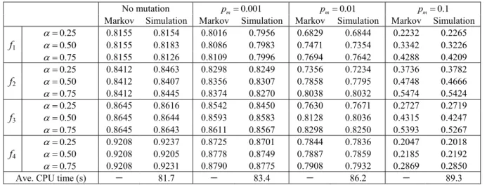
STRATEGYA RESULTS FORTESTPROBLEMSWITHβ=0.25ANDDIFFERENTMUTATIONRATES. THENUMBERS IN THETABLESHOW THEPROPORTION OFOPTIMALINDIVIDUALS IN THEPOPULATION; THATIS,THEFRACTION OF THEPOPULATIONTHAT ISOPTIMAL

randomly-selected individuals. Strategy A does not include recombination or mutation, although it could be modified to include these features. The population of strategy A evolves according to the following two rules.

1) Denote α ∈ [0,1] as the replacement pool probability. Randomly choose round(αN) individuals, where N is the population size. Denoteλj∈[0,1] as the modifica-tion probability. λj is typically chosen as a decreasing function of fitness; that is, good individuals should have a smaller probability of replacement than poor individuals.

2) The jth individual chosen in the previous step, where

j ∈ [1,round(αN)], has a probability of λj of being replaced with one of K individuals from the search space (recall that K is the cardinality of the search space, and {xi : i =1, . . . ,K} is the search space). The probabil-ity of selecting the ith individual xi as a replacement is denoted asμiand is composed of two parts: a)β∈[0,1] is assigned to each individual equally and b) the remain-ing probability 1−βis assigned among the xiindividuals in the proportions (m1, . . . ,mK), where mi is the pro-portion of the xi individuals in the population; that is,

mi is the number of xi individuals in the population divided by the population size. So the probability of selecting xi as a replacement isμi=β/K+(1−β)mi. Note that K_i=1μi = 1. If the selection probability is independent of mi, that is, β = 1, then the prob-ability of selecting xi as a replacement is μi = 1/K for all i.

Algorithm 1 shows an EA that operates according to strategy A. We see from Algorithm 1 that strategy A has four tuning parameters: 1) N (population size); 2) α (replacement pool probability); 3) β (the constant component of the selec-tion probability); and 4) λ(modification probability, which is a function of fitness).

Note that strategy A (Algorithm 1) is not an EA when β = 1; in this case the algorithm is equivalent to a Monte Carlo search strategy in which random candidate

Algorithm 1 EA Based on Strategy A. α and β are Tuning Parameters in the Range [0, 1], λ is a Decreasing Function of Fitness, and K is the Cardinality of the Search Space. The Interactive Markov Model for this Algorithm will be Shown in Section II-D1. The Equilibrium Population of this Algorithm will be Established in Theorem 1

Generate an initial population of individuals Y= {yk: k=1,· · ·,N}

While not (termination criterion)

Randomly choose round(αN)parent individuals

For each chosen parent individual yj( j=1,· · ·,round(αN))

Use modification probability λj to probabilistically

decide whether to replace yj

If replacing yjthen

Select one of the xi(i = 1,· · ·,K), each with

probability [β/K+(1−β)mi]

yj←xi

End replacement Next individual: j←j+1 Next generation

solutions are evaluated. As β → 0 the algorithm becomes more and more evolutionary in the sense that individual fit-ness implicitly drives the algorithm more strongly. TablesII–V show that strategy A performs better asβ →0.

2) Strategy B: The second EA adaptation that we

intro-duce, which we call strategy B, is based on a social process model [25, Example 6]. Strategy B is similar to strategy A in its selection of random individuals from the search space, and the replacement of individuals with those randomly-selected individuals. However, strategy B includes elites. The population of strategy B evolves according to the following two rules.

1) For each individual ykin the population, if yk is the best individual in the search space, there is a probability σ1 that it will be classified as elite, where σ1 ∈ [0,1] is a user-defined tuning parameter.

2) If yk is not classified as elite, use λk to probabilisti-cally decide whether to modify yk. If yk is selected for modification, it is replaced with xi with a probability

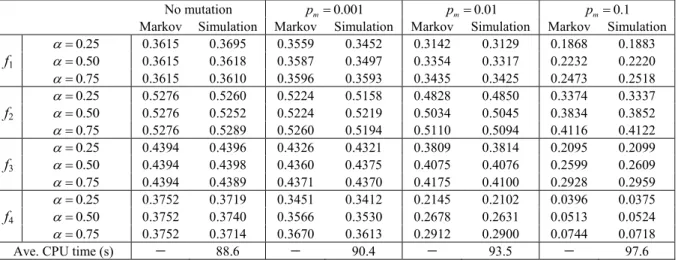
TABLE III

STRATEGYA RESULTS FORTESTPROBLEMSWITHβ=0.5ANDDIFFERENTMUTATIONRATES. THENUMBERS IN THETABLESHOW THEPROPORTION OFOPTIMALINDIVIDUALS IN THEPOPULATION; THATIS,THEFRACTION OF THEPOPULATIONTHATISOPTIMAL

TABLE IV

STRATEGYA RESULTS FORTESTPROBLEMSWITHβ=0.75ANDDIFFERENTMUTATIONRATES. THENUMBERS IN THETABLESHOW THEPROPORTION OFOPTIMALINDIVIDUALS IN THEPOPULATION; THATIS,THEFRACTION OF THEPOPULATIONTHATISOPTIMAL

proportional toα+βmi, where mi is the fraction of the population that is comprised of xi individuals. Recall that {xi : i=1, . . . ,K} is the search space.

Similar to strategy A, strategy B does not include recombi-nation or mutation, although it could be modified to include these features. Algorithm 2 illustrates an EA that operates according to strategy B. We see from Algorithm 2 that strat-egy B has the same four tuning parameters as stratstrat-egy A: 1) N (population size); 2) α (replacement pool probability); 3) β (selection constant); and 4) λ (modification probabil-ity, which is a function of fitness). However, note that α and β are used differently in strategies A and B (that is, in Algorithms 1 and 2).

Note that strategy B (Algorithm 2) is purely random when β = 0. In this case the only role of the fitness values is to decide which individuals to replace. The fitness values do not guide the formation of new individuals since the individu-als that are kept are essentially useless. The same outcome would be provided with a population of a single individual

being replaced every generation by a randomly chosen indi-vidual from the search space. As β → 1 the algorithm becomes more and more evolutionary in that individual fit-ness implicitly drives the algorithm more strongly. Later in the paper, TableVIwill show that strategy B performs better as β→1.

The selection probability of xi in strategy B is

μi≡Pr(yk ←xi)=α+βmi (3) for i∈[1,K]. Equation (3) is the probability that ykis replaced by xi, and this probability is a linear function of mi, which is the proportion of xi individuals in the population. Note that (3) holds for all k∈ [1,N] for which yk is selected for replacement.

3) Selection Pressure in Strategies A and B: The selection

probabilities in strategies A and B are both linear with respect to the fraction of xiindividuals in the population. Fig.1depicts the selection probability.

TABLE V

STRATEGYA RESULTS FORTESTPROBLEMSWITHβ=1ANDDIFFERENTMUTATIONRATES. THENUMBERS IN THETABLESHOW THE PROPORTION OFOPTIMALINDIVIDUALS IN THEPOPULATION; THATIS,THEFRACTION OF THEPOPULATIONTHATISOPTIMAL

Algorithm 2 EA Based on Strategy B. α andβ Are Tuning Parameters in the Range [0, 1], λ is a Decreasing Function of Fitness, and K is the Cardinality of the Search Space. The Interactive Markov Model for This Algorithm Will be Shown in Section II-D2. The Equilibrium Population of this Algorithm will be Established in Theorem 2.

Generate an initial population of individuals Y = {yk: k=1,· · ·,N}

While not (termination criterion) For each individual yk

If ykis not the best individual in the search space then

Use replacement probability λk to decide whether

to replace yk

If replacing ykthen

Select one of the xi(i = 1,· · ·,K), each

with probability [α+βmi] y_k←xi End replacement End if Next individual: k←k+1 Next generation

If the search space cardinality K is greater than the popula-tion size N in Fig. 1, as in practical EA implementations, then min(mi) = 0. This is because there are not enough individuals in the population to cover the search space, so there are some search space individuals xi that are not in the population Y.

If selection is overly-biased toward populous individuals, the EA may converge quickly to a uniform population while not widely exploring the search space. If selection is not biased strongly toward populous individuals, the population will be more scattered with fewer good individuals. Note that the most populous individuals will be the ones with highest fitness if we define modification probability λk as a decreas-ing function of fitness. We will see this effect in our results in Section IV.

A useful metric for quantifying the difference between various selection methods is selection pressure φ, which is

Fig. 1. Selection probability in strategies A and B. The min and max oper-ators are taken over i ∈ [1,K], where K is the cardinality of the search space.

defined as follows [4, p. 34]:

φ= max(Pr(selection))

average(Pr(selection)) (4) where Pr(selection) is the probability that an individual is selected to replace another individual.

The most populous individual has the fraction max(mi) individuals, which we denote as mmax. Since selection prob-ability is affine (Fig. 1), average selection probability is an affine function of (max(mi)+min(mi))/2 =mmax/2, assum-ing K > N, as discussed earlier. In this case the selection

pressure of strategy B can be calculated from (4) as φ= α+βmmax

α+βmmax/2

. (5)

If we normalize the selection probabilities to sum to 1, we get K i₌1 Pr(yk←xi)= K i₌1 (α+βmi) =Kα+β K i=1 mi=Kα+β=1 (6)

TABLE VI

STRATEGYB RESULTS FORTESTPROBLEMf1. THENUMBERS IN THETABLESHOW THEPROPORTION OFOPTIMAL INDIVIDUALS IN THEPOPULATION; THATIS,THEFRACTION OF THEPOPULATIONTHATISOPTIMAL

where we used the fact thatK_i=1mi=1 since the sum of the fractions must equal 1. If we desire a given selection pressure we can solve (5) and (6) forα andβ to obtain

α= mmax(2−φ)

Kmmax(2−φ)+2(φ−1)

β = 2(φ−1)

Kmmax(2−φ)+2(φ−1).

(7)

Note that (7) also holds for strategy A (Algorithm 1) ifα is replaced with β/K, and β is replaced with(1−β).

C. Convergence

We begin this section with a preliminary theorem of the convergence conditions of interactive Markov models.

Theorem 1: Consider an interactive Markov model in the

form of (1). If there exists a positive integer R such that

R

t=1P[m(t)] is positive definite for all m(t) ≥ 0 such that

K

i=1mi(t) = 1, where t = 1,2, . . . ,R, then

R

t=1P[m(t)] converges as R→ 8 to a steady state which has all nonzero entries.

Proof: See [26] for a proof and discussion.

Later in this section, we will use Theorem 1 to show that there is a unique limiting distribution for the states of the interactive Markov models in strategies A and B. We will also show that the probability of each state of the model is nonzero at all generations after the first one. Theorem 1 will show that Algorithms 1 and 2 have a unique limiting distribution with nonzero probabilities for each point in the search space. This implies that Algorithms 1 and 2 will both eventually find the globally optimal solution to a discrete optimization problem.

D. Interactive Markov Model Transition Matrices

The previous sections presented two simple EA adapta-tions and showed that they both have a unique population distribution as the generation count approaches infinity. Now we analyze their interactive Markov models in more detail and find explicit solutions to the steady-state population distributions. Firstly, we discuss strategy A.

1) Interactive Markov Model for Strategy A:

a) Selection: We can use [25, Example 1] to obtain the

following interactive Markov model of strategy A:

pij= ( 1−α)+α1−λj +λj β/K+(1−β)mj if i=j αλj(β/K+(1−β)mi) if i=j (8) for (i, j)∈[1, K]. pij is the probability that a given individual in the population transitions from xj to xi in one generation.

The first equality in (8), when i=j, denotes the probability

that an individual does not change from one generation to the next. This probability is composed of three parts.

1) The first term, 1−α, is the probability that the individual is not selected for the replacement pool.

2) The first part of the second term is the product of the probability that the individual is selected for the replace-ment pool (α), and the probability that the individual is not selected for modification (1−λj).

3) The second part of the second term is the product of the probability that the individual is selected for the replacement pool (α), the probability that the individual is selected for modification (λj), and the probabil-ity that the selected individual is replaced with itself (β/K+(1−β)mj).

The second equality in (8), when i=j, is the probability that

an individual is changed from one generation to the next. This probability is similar to the second part of the second term of the first equality as discussed in 3) above, the difference being that mi is used instead of mj because the selected individual is changed from xj to xi.

b) Mutation: Next we add mutation to the interactive

Markov model of strategy A. Typically EA mutation is imple-mented by probabilistically complementing each bit in each individual. Then the probability that xi mutates to xk can be written as

pki=Pr(xi→xk) =pmHik(1−pm)q−Hik (9) where pm ∈ (0, 1) is the mutation rate, q is the number of bits in each individual, and Hij is Hamming distance between

pkj= i pkipij = ⎧ ⎪ ⎪ ⎪ ⎪ ⎨ ⎪ ⎪ ⎪ ⎪ ⎩ 1−(K−1)pm K (1−α)+α 1−(K−1)pm K 1−λj +λj 1−(K−1)pm K β K+ (K−1)pm K2 β+ pm K(1−β)+(1−β)(1−pm)mj if k=j pm K(1−α)+α pm K 1−λj +λj 1−(K−1)pm K β K + (K−1)pm K2 β+ pm K(1−β)+(1−β)(1−pm)mk if k=j (11) akj= ⎧ ⎪ ⎪ ⎪ ⎨ ⎪ ⎪ ⎪ ⎩ 1−(K−1)pm K (1−α)+α 1−(K−1)pm K 1−λj +λj 1−(K−1)pm K β K+ (K−1)pm K2 β+ pm K(1−β) if k=j pm K(1−α)+α pm K 1−λj +λj 1−(K−1)pm K _β K + (K−1)pm K2 β+ pm K(1−β) if k=j bkj=αλj(1−β)(1−pm) (12)

But with single-bit mutation, the transition matrix elements

pkj =

ipkipij would not satisfy the form of (2) and (8). So we use a modified mutation operator that randomly replaces an entire individual rather than a single bit of an individual. Mutation of the jth individual is implemented as follows.

For each individual yj If rand(0, 1)<pm

yj←rand(L, U) End if

Next individual

In the above mutation (replacement) logic, rand(L, U) is a uniformly distributed random number between L and U, and L and U are the lower and upper bounds of the search space. The above logic replaces each individual with prob-ability pm. The descriptions of strategies A and B with mutation are the same as Algorithms 1 and 2 except that we add the above replacement logic at the end of each gener-ation. Note that replacement acts equally on all individuals

Y = {yk : k=1, . . . ,N}. In strategy B, we use elitism to prevent selection but not to prevent replacement.

The transition probability of the modified mutation (replace-ment) operator is described as follows:

pki = (1−pm)+pm/K if k=i

pm/K if k=i. (10)

Then the transition probability of strategy A with mutation, and the corresponding A and B matrices in (2) can be written as (11) and (12), shown at the top of this page.

The derivation of (11) and (12) is in the Appendix. Now we are in a position to state the main result of this section.

Theorem 2: The K×1 equilibrium population fraction vector

m* of Algorithm 1, which is exactly modeled by the

interac-tive Markov model of (1) and (11), is equal to the dominant eigenvector (normalized so its elements sum to one) of the matrix A0 =akj/(bj+K_i=1aij), where akj is given by (12), and bj is shorthand notation for bkj in (12) since all the rows of B are the same.

Proof: This theorem derives from [25, Th. 1]. We provide

the proof in the Appendix.

Next we consider the special caseμi=1/K in Algorithm 1. In this case the transition probability of (11) is written as

pkj= ⎧ ⎪ ⎪ ⎪ ⎪ ⎨ ⎪ ⎪ ⎪ ⎪ ⎩ 1−(K−1)pm K (1−α)+α 1−(K−1)pm K 1−λj +λj K if k=j pm K(1−α)+α _p m K 1−λj +λj K if k=j (13) which is independent of mi; that is, the interactive Markov model reduces to a standard noninteractive Markov model. In this case we can use [25, Th. 1] or standard noninterac-tive Markov theory [18] to obtain the equilibrium population fraction vector m*.

2) Interactive Markov Model for Strategy B: Before

dis-cussing the interactive Markov model of strategy B, we define some notation. Suppose thatσ =[σk] denotes the fraction of individuals that always remain equal to xkfor each k∈[1, K]. Thenkσkis the fraction of all individuals that never change. We call these individuals stayers. In an EA, the stayers are comprised of a user-specified fraction of the best individu-als in the population. Vector n=[n1, . . . ,nK] consists of the fractions of all individuals that are allowed to change, and we call these individuals movers. m =[m1, . . . ,mK] is the frac-tion of all individuals in the populafrac-tion. The fracfrac-tion of xj individuals thus includes two parts: 1) σj, which is the frac-tion of all xj individuals that are not allowed to change and 2)(1−K_k=1σk)nj, which is the fraction of all xjindividuals that may change in future generations. So the fraction vector

m is given by m=σ+ 1− K k=1 σk n. (14)

Theσ vector is related to EA elitism since it defines the pro-portion of individuals in the population that are not allowed to change in subsequent generations. One common approach to elitism is to prevent only optimal-enough individuals from changing in future generations [17]. That is, σ1>0 (assum-ing without loss of generality that x1 is the optimal point in the search space), andσk=0 for all k >1. In this case (14) becomes

mi= ₍σ1+(1−σ1)n1 for i=1, the optimal state 1−σ1)ni for i=1, nonoptimal states. (15)

pij = ⎧ ⎪ ⎪ ⎨ ⎪ ⎪ ⎩

(1−λ1)+λ1[α+β(σ1+(1−σ1)n1)] if i=j=1,which is the best state

λj[α+β(σ1+(1−σ1)n1)] if i=1 and j=1 1−λj +λj[α+β(1−σ1)ni] if i=j=1 λj[α+β(1−σ1)ni] if i=j,and i=1 (16)

Strategy B elitism is a little different than standard EA elitism. In strategy B we assume that we know whether or not an individual has acceptable performance in the judgment of the decision maker. This is not always the case in practice, but it may be the case for certain problems. For example, suppose we are trying to solve a state estimation problem. In this case, the Cramer–Rao bound gives a lower bound on the estimation error, along with conditions that tell us if such an estima-tor exists, but does not tell us what estimaestima-tor achieves the lower bound [27]. An engineer may also know ahead of time the acceptable performance for an estimator, regardless of the Cramer–Rao bound. The same situations arise with the per-formance bounds and design of H2 and H∞controllers [28]. As another example, if the fitness of a product design is mea-sured by the qualitative judgments of test subjects, we might know ahead of time that a rating of 9 out of 10 is accept-ably optimal, although we might not know how to achieve that rating.

If S individuals at the global optimum are retained as elites, then σ1 = S/N (this quantity could change from one gener-ation to the next). If N1 individuals at the global optimum are allowed to change, then n1=N1/(N−S). Multiple indi-viduals at the global optimum could mean that there are duplicate individuals in the population, or it could mean that there are multiple solutions to the optimization problem. If an individual is not globally optimal, then we must always allow it to change—that is, we can implement elitism only for individuals that are globally optimal. Even if we have globally optimal individuals in the population, we may want to continue the search. This is because other solutions near (but not at) the global optimum may have desirable proper-ties. To return to our previous example, an estimator with an error larger than the lower bound may be more desirable than one at the lower bound if the first estimator is more robust. Similarly, a product rating less than perfect might be more desirable than one with a perfect rating because of other factors.

Example: To clarify the relationships betweenσ, n, and m, we present a simple example. Suppose we have a population of 14 individuals, and the search space size is 3; that is, N=14 and K=3. Then:

1) two individuals in state 1 are stayers (they will never leave state 1);

2) three individuals in state 1 are movers (they may transition out of state 1);

3) four individuals are in state 2, and they are all movers; 4) five individuals are in state 3, and they are all movers. Therefore:

1) n1=3/12 (fraction of movers that are in state 1); 2) σ1 = 2/14 (fraction of population that are stayers in

state 1);

3) n2=4/12 (fraction of movers that are in state 2); 4) n3=5/12 (fraction of movers that are in state 3). In this example, we have assumed that the engineer has specified that the best 2/14 of the population will be stayers and that the rest of the population will be movers. We sub-stitute these values in (15) and obtain m1 = 5/14 (fraction of individuals that are in state 1), m2 = 4/14 (fraction of individuals that are in state 2), and m3 = 5/14 (fraction of individuals that are in state 3), which are the same as the distributions stated at the beginning of this example.

a) Summary of the interactive Markov model for strategy B: Now we use [25, Example 6], combined with (6) above, to obtain the following interactive Markov model of strategy B selection.

Equation (16), as shown at the top of this page, can be explained as follows. For the first equality, when i= j =1, which is the best state, the transition probability includes two parts: 1) the first term, which denotes the probability that the individuals is not changed (1−λ1) and 2) the second term, which denotes the probability that the individual is changed to itself, and which is the product of the probability that the individual is changed (λ1), and the probability that the selected

xiterm is equal toλ1(μ1/

K

k=1μk). This second term can be written as λ1_Kμ1 k=1μk =λ1 α+β m1 K k=1(α+βmk) =λ1α+β(σ 1+(1−σ1)n1) Kα+β =λ1(α+β(σ1+(1−σ1)n1)). (17) The third equality in (16), for i=j=1, is the same as the first equality, except thatσ1+(1−σ1)njis replaced with(1−σ1)nj as indicated by (15). In the second equality in (16), when i=1 (corresponding to the best state) and j=1 (corresponding to a suboptimal state), the transition probability only includes the probability that the individuals is changed, which is the same as the second term in the first equality. Finally, the fourth equality in (16) is the same as the second equality, except that σ1+(1−σ1)njis replaced with(1−σ1)njsince i=1 (that is,

xi is not the best state), as indicated by (15).

By incorporating the modified mutation probability described in (10), we obtain the transition probability of strat-egy B with mutation. The A and B matrices shown in (2) can be derived as shown in the Appendix and can be written as (18) and (19), shown at the top of next page.

Theorem 3: Assume that the search space has a single global

optimum. Then the K×1 equilibrium fraction vector of movers

n* of Algorithm 2, which is exactly modeled by the interactive

Markov model of (1) and (18), is equal to the dominant eigen-vector (normalized so its elements sum to one) of the matrix

pkj = i pkipij = ⎧ ⎪ ⎪ ⎪ ⎪ ⎨ ⎪ ⎪ ⎪ ⎪ ⎩

pm/K+(1−pm)[(1−λ1)+λ1(α+β(σ1+(1−σ1)n1))] if k=j=1, which is the best state

pm/K+(1−pm) λj(α+β(σ1+(1−σ1)n1)) if k=1 and j=1 pm/K+(1−pm) 1−λj +λj(α+β(1−σ1)nk) if k=j=1 pm/K+(1−pm) λj(α+β(1−σ1)nk) if k=j, and k=1 (18) akj = ⎧ ⎪ ⎪ ⎪ ⎪ ⎨ ⎪ ⎪ ⎪ ⎪ ⎩

pm/K+(1−pm)[(1−λ1)+λ1(α+βσ1)] if k=j=1, which is the best state

pm/K+(1−pm) λj(α+βσ1) if k=1 and j=1 pm/K+(1−pm) 1−λj +λjα if k=j=1 pm/K+(1−pm) λjα if k=j, and k=1 bkj =(1−pm)λjβ(1−σ1) (19)

shorthand notation for bkj in (19) since all the rows of B are the same. Furthermore, the equilibrium fraction vector m* is obtained by substituting n* in (15).

Proof: The proof of Theorem 3 is analogous to that of

Theorem 2, which is given in the Appendix.

E. Computational Complexity

The computational cost of Algorithms 1 and 2, like most other EAs, is dominated by the computational cost of the fitness function, which is computed for each individual in the population once per generation. Therefore, the compu-tational costs of Algorithms 1 and 2 are of the same order as any other EA that uses a typical selection–evaluation-recombination strategy. Algorithms 1 and 2 also require a roulette-wheel process to select the replacement individ-ual (xi in Algorithms 1 and 2), which requires effort of the order K2, but that computational cost can be greatly reduced by using linear ranking [17, Sec. 8.7.5].

The computational cost of the interactive Markov model calculations requires the formation of the transition matrix components, which is (12) for Algorithm 1 and (19) for Algorithm 2. After the transition matrix is computed, the dominant eigenvector of a certain matrix needs to be com-puted to calculate the equilibrium population, as stated in Theorems 2 and 3. There are many methods for calculating eigenvectors, most of which have a computational cost of the order K3, where K is the order of the matrix and is equal to the cardinality of the search space.

In summary, using the interactive Markov chain model to calculate an equilibrium population requires three steps: 1) cal-culation of the transition matrix components, as shown in (12) for Algorithm 1 and (19) for Algorithm 2; 2) formation of a certain matrix, as shown in Theorem 2 for Algorithm 1 and Theorem 3 for Algorithm 2; and 3) calculation of a dominant eigenvector, as described in Theorem 2 for Algorithm 1 and Theorem 3 for Algorithm 2. The eigenvector calculation dom-inates the computational effort of these three steps, and is of the order K3.

The above analysis is a per-generation analysis. In prac-tice, an EA runs for a certain number of generations before termination. Per-generation run time is not meaningful unless

a convergence rate can be established. Section II-C guarantees convergence for Algorithms 1 and 2, but does not establish the convergence rate. Future work could explore the convergence rate of the algorithms, perhaps using Markov process-based approaches [29] or run-time analysis [30].

III. SIMILARITIES OFEAS

In this section, we first compare strategies A and B as shown in Algorithms 1 and 2. Note that we only consider selection here. If the replacement pool probability α = 1 in strategy A, then it reduces to strategy B if elitism is not used (σ1 = 0). Although the probability of selection of xi in the two strategies appears different, they are essentially the same because they both use a selection probability that is a linear function of the fractions of the xiindividuals in the population.

Next we discuss the equivalence of strategy B, and a GA with global uniform recombination (GA/GUR) and elitism with no mutation as described in [31, Fig. 3]. Strategy B and GA/GUR are equivalent under the following circumstances.

1) In GA/GUR we replace an entire individual instead of only one decision variable at a time.

2) In GA/GUR we use a selection probability that is pro-portional to the fractions of individuals in the population. 3) In strategy B we use modification probabilityλk=1. This implementation of GA/GUR is also called the Holland algorithm [32] and is shown in Algorithm 3. Note that some researchers would not consider GA/GUR as a genuine GA since it does not include classical crossover. It might instead be more correctly referred to as “EA/GUR.” However, we retain the GA/GUR terminology here for consistency with previous work [31].

Next we discuss the equivalence of strategy B and BBO with elitism and no mutation [13]. BBO is an EA that is inspired by the migration of species between islands and is described by [31, Fig. 2]. BBO involves the migration of decision vari-ables between individuals in an EA population. If we allow migration of entire individuals instead of decision variables, and if we set the BBO emigration probability proportional to the fractions of individuals in the population, then BBO

Algorithm 3 Genetic Algorithm With Global Uniform Recombination (GA/GUR) With Selection Probability Proportional to the Fractions of Individuals in the Population. This is Equivalent to Strategy B in Algorithm 2 ifλk = 1 for all k.

Generate an initial population of individuals Y = {y_k: k=1,· · ·,N}

While not (termination criterion) For each individual y_k

If y_kis not the best individual in the search space then Use population proportions to probabilistically select

xi, i∈[1, K]

yk ←xi

End if

Next individual: k ←k+1

Next generation

Algorithm 4 Biogeography-Based Optimization (BBO) With Global Migration and With Selection Probability Proportional to the Fractions of Individuals in the Population. This is Equivalent to Strategy B in Algorithm 2

Generate an initial population of individuals Y = {y_k: k=1,· · ·,N}

While not (termination criterion) For each individual yk

If yk is not the best individual in the search space then

Use λkto probabilistically decide whether to immigrate

to yk

If immigrating then

Use population proportions to probabilistically select

xi,i∈[1,K] yk←xi End immigration End if Next individual: k←k+1 Next generation

becomes equivalent to EA strategy B. Algorithm 4 shows this modified version of BBO.

There are many other EAs that are equivalent to each other under special circumstances [33] and so they may also be equivalent to strategies A or B under certain conditions. We leave this study to future research.

IV. SIMULATIONRESULTS ANDCOMPARISONS In the following, Sections IV-A and IV-B confirm the interactive Markov model theory of Section II with simula-tion results, and investigate the effects of tuning parameters on strategies A and B. Section IV-C compares population-proportional selection with two standard EAs (GA and BBO) on a set of real-world benchmark problems.

A. Strategy A—Confirmation of Interactive Markov Model

In strategy A (Algorithm 1), the main tuning parameters are the replacement pool probability α, and the parameter β of the selection probabilityβ/K+(1−β)mi. We use the fraction

m∗_bof how many individuals are equal to the optimum to com-pare performances with different tuning parameters. A larger fraction m∗_b indicates better performance.

The first three test functions have a search space cardinality of K = 8; that is, they are three-bit problems with fitness functions that correspond to bit strings (0 0 0), (0 0 1), (0 1 0),

(0 1 1), (1 0 0), (1 0 1), (1 1 0), and (1 1 1). These three fitness functions are given as follows:

f1= 1 2 2 3 2 3 3 4 f2= 4 2 2 3 2 3 3 4 f3= 4 1 1 2 1 2 2 3. (20)

These functions are chosen as representative functions because

f1is a unimodal one-max problem, f2is a multimodal problem, and f3 is a deceptive problem. Note that all three of these problems are maximization problems.

We also use the multimodal Ackley function with 20 dimen-sions to confirm the interactive Markov model of strategy A. The Ackley function is described as follows:

f4= −20 exp ⎛ ⎝₋0.2 n i=1x2i n ⎞ ⎠ −exp n i=1cos(2πxi) n +20+e, −30≤xi≤30. (21) The granularity or precision of each independent variable is set to 1 here to allow for experimental confirmation of the interactive Markov model theory while still providing for rea-sonable computational effort. Note that the Ackley function is a minimization problem.

We useα=0.25,0.50,0.75 andβ=0.25,0.50,0.75, with modification probabilitiesλi=1−fitness(xi), where fitness(xi) denotes the fitness value of individual xi, which is normalized to the range [0,1]. We use population size = 50, genera-tion limit =20 000, and 30 Monte Carlo runs for each test. TablesII–IVshow comparisons between theoretical interactive Markov results (Theorem 2 in Section II) and strategy A simu-lation results. TableVshows similar comparisons for strategy A for the special caseβ=1, which gives selection probability μi=1/K for all i, independent of population fractions. The results in TablesII–Vcan be reproduced with MATLAB code that is available at the authors’ Web site [34].

The numbers in the tables show the proportion of optimal individuals in the population. For example, the optimal indi-vidual for function f1is [1,1,1]. The first entry in TableII(α =0.25, no mutation) shows the number 0.8155, which means that 81.55% of the population is comprised of the bit string [1,1,1].

Note that the purpose of Tables II–V is not to show the superiority of one algorithm over another, or of one set of tuning parameters over another. The purpose is rather to show that simulation results confirm the theoretical Markov results. Note first from Tables II−V that the parent selection proba-bility α does not affect the proportion of individuals in the population in the case of no mutation. This is because α divides out of the m∗=P(m∗)m∗equilibrium equation in this case. The finding is consistent with [25, p. 162]. However, we see that αcan slightly affect the proportion of individuals in the case of nonzero mutation.

Second, for a given replacement pool probability α and parameter β, the proportion of optimal individuals decreases

with increasing pm. This indicates that low mutation rates have better performance. A high mutation rate of 0.1 results in too much exploration and the population remains too widely distributed across the search space.

Third, for a given replacement pool probabilityαand muta-tion rate pm, the propormuta-tion of optimal individuals decreases with increasingβ. This is because the modification probability λi tends to result in a population in which good individu-als dominate, and increasing β causes individuals with high populations to be more likely to replace other individuals.

Fourth, Tables II–V show that the interactive Markov model results and the simulation results match well for all test problems, which confirms the interactive Markov model theory.

Fifth, the average CPU times in the last rows of TablesII–V show the simulation times for the four test problems. Strategy A runs faster with smaller mutation rates. The rea-son is that larger mutation rates require more mutations, which slightly increases computation time. However, in real-world problems, computational effort is dominated by fitness function evaluation, which is independent of the mutation rate.

B. Strategy B—Confirmation of Interactive Markov Model

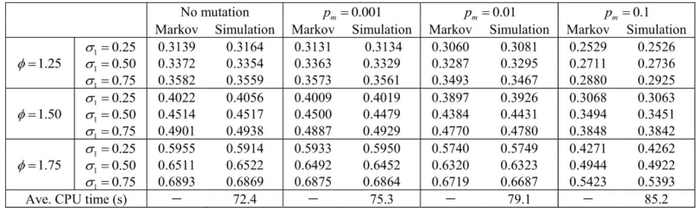
In this section, we investigate the effect of selection pres-sureφ, which influences the selection probabilityα+βmiof xi in strategy B, as shown in (7). In this section, we test only the unimodal one-max problem f1 (Theorem 3 assumes that the optimization problem is unimodal). Recall that EA selection pressure is constrained to the domain φ ∈ (1,2) [4, p. 34]. In this section, we test φ = 1.25,1.50,1.75 in (7) to com-pute parameters α, β of the selection probability, and we test elitism probabilitiesσ1=0.25,0.50,0.75. The other parame-ters of the EA are the same as in the previous section. TableVI shows comparisons between interactive Markov theory results and strategy B simulation results. The results in Table VIcan be reproduced with MATLAB code that is available at the authors’ Web site [34].

Note first from Table VI that for a given value of elitism probability σ1 and mutation rate pm, performance improves as selection pressure φ increases. This is expected because a larger value ofφ exploits more information from the popu-lation. For a more complicated problem with a larger search space, we might arrive at different conclusions about the effect of φ on performance.

Second, for a given value of selection pressureφand muta-tion rate pm, performance improves as elitism probability σ1 increases. Again, this is expected for simple problems such as the test problem studied in this section, but the conclusion may not hold for more complicated problems.

Third, for a given value of elitism probabilityσ1and selec-tion pressure φ, performance improves as mutation rate pm decreases. This again indicates that low mutation rates give better performance for the test problems that we study. A high mutation rate of 0.1 results in too much exploration, and the population remains too widely distributed.

Fourth, we see that the interactive Markov model theory and the simulation results match well, which validates the theory.

TABLE VII

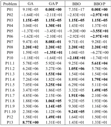
REAL-WORLDBENCHMARKRESULTS. THE“/P” VERSION OFEACH ALGORITHM IS THEPOPULATION-PROPORTION-SELECTION MODIFICATION OF THEALGORITHM. THENUMBERSSHOW THEMEANVALUE OF25 INDEPENDENTSIMULATIONS. THEBESTRESULT INEACHROWISSHOWN INBOLDFONT

Fifth, we see that strategy B runs faster with smaller muta-tion rates (the same observamuta-tion we made for strategy A in TablesII–V). The reason is that larger mutation rates result in more mutations, which slightly increases computation time.

C. Comparisons on Real-World Benchmarks

This section uses real-world optimization problems from the 2011 IEEE Congress on Evolutionary Computation (CEC) [35] to compare population-proportional selection GA and BBO (Algorithms 3 and 4) with standard GA and BBO. For the modified EAs with population-proportion-based selection, we use selection probability (α+βmi), where midenotes the frac-tion of xi individuals in the population. For the GAs we use real coding, roulette wheel selection, single-point crossover with a crossover probability of 1, and a mutation probability of 0.001. For BBO we use maximum immigration and emi-gration rates of 1, linear miemi-gration curves [13], and a mutation probability of 0. Each algorithm uses a population size of 50, an elitism size of 2, and a fitness function evaluation limit of 100 000.

Algorithm 3 is equivalent to a GA with population-proportional selection (GA/P), and Algorithm 4 is equiva-lent to BBO with population-proportional selection (BBO/P). These equivalences motivate us to compare GA with GA/P, and BBO with BBO/P. The only difference between standard GA and GA/P in this section is that standard GA uses fitness-based selection while GA/P uses population-fitness-based selection.

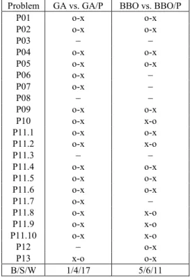
TABLE VIII

WILCOXONTESTRESULTS FORPAIR-WISEALGORITHMCOMPARISONS. IF THEDIFFERENCEBETWEEN THEALGORITHMS ISSTATISTICALLY SIGNIFICANT,THEPAIRS AREMARKED ASFOLLOWS: “X-O” SHOWS THAT THELEFTALGORITHM ISBETTERTHAN THERIGHTONE;

“O-X” SHOWSTHAT THERIGHTALGORITHM ISBETTERTHAN THELEFTONE. THEB/S/W ROW AT THEBOTTOMSHOWS THE TOTALSCORES, WHERE“B” DENOTES THENUMBER OFTIMES THELEFTALGORITHMPERFORMSBETTER, “S” DENOTES THENUMBER OFTIMES THETWOALGORITHMSPERFORM

THESAME,AND“W” DENOTES THENUMBER OF TIMES THELEFTALGORITHMPERFORMS

WORSETHAN THERIGHTONE

Similarly, the only difference between standard BBO and BBO/P in this section is that standard BBO uses fitness-based selection while BBO/P uses population-based selection.

TableVIIsummarizes the performances of the EAs on the real-world optimization problems. All results are averages of 25 independent simulations. The performance data in TableVII for standard GA and BBO is taken from [33]. Computational time is the same for standard GA and GA/P, and is the same for standard BBO and BBO/P. This is because the algorithms execute identically except for the difference between fitness-based selection and population-fitness-based selection.

We use the Wilcoxon method to test for statistical significance [36]. The Wilcoxon test results are shown in Table VIII, where a pair is marked if the difference between the pair of algorithms is statistically significant.

The results in Table VIII are divided into the GA versus GA/P group, and the BBO versus BBO/P group. For each pair of algorithms we calculate B/S/W scores, where “B” denotes the number of times that the left algorithm performs better than the right one, “S” denotes the number of times that the left algorithm performs statistically the same as the right, and “W” denotes the number of times that the left algorithm performs worse than the right one.

TableVIIIshows that for GA versus GA/P, the B/S/W score is 1/4/17, which indicates that GA outperforms GA/P one time, GA is statistically the same as GA/P four times, and GA/P outperforms GA 17 times. For BBO versus BBO/P, the B/S/W score is 6/5/11, which indicates that BBO outperforms BBO/P six times, BBO is statistically the same as BBO/P five times, and BBO/P outperforms BBO 11 times. Population-proportion-based EAs significantly outperform standard EAs on the CEC 2011 real-world problems.

V. CONCLUSION

This paper first presented a formal interactive Markov model, which involves separate but interacting Markov models for each individual in an EA population. Then we proposed two simple optimization search strategies whose basic features are population-proportion-based selection and modified muta-tion, which we called population-proportion-based EAs, and analyzed them exactly with interactive Markov models. The theoretical results were confirmed with simulation results, and showed how the interactive Markov model can describe the convergence of the EAs. The theoretical and simulation results in Tables II–VI can be reproduced with MATLAB code that is available at the authors’ Web site [34]. TablesVIIandVIII showed that GA and BBO perform better on real-world benchmark problems if population-proportion-based selection is used.

The use of interactive Markov models to model EAs can lead to useful conclusions. Interactive Markov models prove to be tractable for much larger search spaces and populations than noninteractive Markov models.

The noninteractive (standard) Markov model has a state space whose dimension grows factorially with search space cardinality and population size, while the interactive Markov model has a state space whose dimension grows linearly with the cardinality of the search space, and is independent of population size. Like the noninteractive Markov model, the interactive Markov model provides exact models for the behav-ior of the EA. Interactive Markov models can be studied as functions of EA tuning parameters to predict their impact on EA performance, and to provide real-time adaptation. Just as noninteractive Markov models have led to the develop-ment of dynamic system models, the same could happen with interactive Markov models. Although the interactive Markov models in this paper explicitly provide only steady-state prob-abilities, they might also be used to understand transient EA behavior and to obtain the probability of optimum-hitting each generation, and to obtain expected hitting times. We see some research in this direction for noninteractive Markov models [37]–[39]; such results are impractical for real-world problems due to the large transition matrices of noninterac-tive Markov models, but such a limitation will not be as great a concern for interactive Markov models.

For future work beyond the suggestions listed above, we see several important directions. First, the interactive Markov model analysis of this paper was based on two simple EAs; future work should explore how to apply the model to other EAs. Second, we used two examples