A Hierarchical Mamdani-Type Fuzzy Modelling Approach with New Training Data Selection and Multi-Objective Optimisation Mechanisms: a Special
Application for the Prediction of Mechanical Properties of Alloy Steels Qian Zhang and Mahdi Mahfouf
Department of Automatic Control and Systems Engineering, The University of Sheffield,
Mappin Street, Sheffield, S1 3JD,
United Kingdom
E-mail addresses: [email protected]; [email protected]
Abstract:
In this paper, a systematic data-driven fuzzy modelling methodology is proposed, which allows to construct Mamdani fuzzy models considering both accuracy (precision) and transparency (interpretability) of fuzzy systems. The new methodology employs a fast hierarchical clustering algorithm to generate an initial fuzzy model efficiently; a training data selection mechanism is developed to identify appropriate and efficient data as learning samples; a high-performance Particle Swarm Optimisation (PSO) based multi-objective optimisation mechanism is developed to further improve the fuzzy model in terms of both the structure and the parameters; and a new tolerance analysis method is proposed to derive the confidence bands relating to the final elicited models. This proposed modelling approach is evaluated using two benchmark problems and is shown to outperform other modelling approaches. Furthermore, the proposed approach is successfully applied to complex high-dimensional modelling problems for manufacturing of alloy steels, using ‘real’ industrial data. These problems concern the prediction of the mechanical properties of alloy steels by correlating them with the heat treatment process conditions as well as the weight percentages of the chemical compositions.
Keywords: Fuzzy; Modeling; Interpretability; Hierarchical clustering; Data selection;
Multi-objective optimization; Particle swarm optimization; Confidence band; Mechanical property, Steel
1 Introduction
There are many modelling problems for which accurate mathematical models do not exist or are difficult to obtain for complex environments [1], and yet the available data that represent the input-output relationships may be abundant. In these cases, alternative data-driven modelling techniques, such as those associated with fuzzy systems, may be suitable techniques to represent related system responses and
behaviours.
In material engineering, it is essential to establish accurate and reliable mechanical property prediction models for materials design and development. But it may be ‘tricky’ to precisely describe the behaviour of mechanical properties using mathematical models alone due to the complexity of materials’ chemical composites and their underlying physical processing mechanisms, such as hot rolling and heat treatment. Thus, developing a fast, efficient and transparent data-driven modelling framework for material property prediction is still a priority.
In the past, some prediction models relating to mechanical properties or manufacturing processes were developed, which were mainly based on linear regression methods [2], fuzzy regression methods [3, 4] or artificial neural networks [5, 6]. Such linear models are only designed for specific classes of steels and specific processing routes, and are not sophisticated enough to account for more complex interactions, while neural networks are black-box techniques and the knowledge behind this kind of models cannot be understood fully. In recent years, fuzzy modelling techniques were also introduced for the prediction of mechanical properties, for instance in [7, 8], but all these attempts did not include multi-objective optimisation as the core solution provider.
Particularly in this work, several important mechanical properties of heat-treated alloy steels were studied, including the Ultimate Tensile Strength (UTS), elongation and Charpy impact energy. These problems are high-dimension modelling problems and have no less than fifteen input variables, which include the weight percentages for various chemical composites as well as the processing parameters of the heat treatment. Moreover, these problems are associated with a large amount of industrial data, which are not well-distributed and may be quantitatively redundant for training purposes. Thus, a training data selection mechanism is needed to find the most appropriate representative data so as to improve the modelling efficiency as well as to reduce computational complexity.
Based on the above consideration, a systematic data-driven fuzzy modelling methodology is proposed in this paper. The most important features of this approach consist of the following:
1. Mamdani fuzzy models [9], instead of TSK fuzzy models [10] (less transparent), are used in the context of the regression problems where precise predictions are needed.
2. A new version of the agglomerative complete-link clustering algorithm [11] is employed to generate the initial fuzzy model. It can reduce the computational complexity and is shown to outperform the well-known clustering algorithm FCM [12].
3. A new data selection technique is proposed for selecting the appropriate and representative data for training. By using this technique, the modelling efficiency can be improved significantly.
4. The multi-objective optimisation technique is employed to improve the modelling performance, taking into account both the accuracy and the interpretability attributes of fuzzy models. As a result, a set of Pareto-optimal fuzzy models with different accuracy and interpretability levels can be generated, which provide a wider choice of different solutions to users.
5. A novel and efficient evolutionary technique, an improved version of PSO [13, 14], is employed in order to optimise both the parameters and the structure of fuzzy systems, which is shown to work effectively in optimising the complex modelling problems.
6. The proposed fuzzy modelling approach is developed to solve not only low-dimensional modelling problems but also challenging high-low-dimensional modelling problems. In this work, all the proposed high-performance paradigms cooperate together in a ‘symbiosis-like’ fashion to tackle the high-dimensional modelling problem efficiently.
7. A new analytical method is proposed for deriving the confidence bands relating to the elicited models. This method can help provide useful information about how confident one can be when analysing an output prediction.
This paper is organised as follows. Section 2 introduces details of the proposed modelling framework. In Section 3, the related experimental studies are presented. First, the proposed modelling approach is applied to the modelling of two benchmark problems, one is a problem of static nonlinear system approximation and the other is a dynamical system identification problem. Furthermore, the modelling framework is applied to the modelling of the mechanical properties of alloy steels using real industrial data. Finally, Section 4 concludes this paper.
2. The proposed modelling methodology
The fundamental concept of fuzzy systems was first introduced by Zadeh in 1965 [15] and later expanded upon in 1973 [16]. The main advantages of fuzzy systems consist of the following: First, fuzzy systems are interpretable (transparent). They include an explicit knowledge representation in the form of linguistic ‘If-Then’ rules, which can easily be understood and explained by humans to allow them to gain a deeper insight into uncertain, complex and ill-defined systems. Second, fuzzy systems are, more often than not, viewed as robust ‘universal approximators’ [17] capable of performing nonlinear mappings between inputs and outputs. Last, fuzzy systems are relatively easy to design and relatively inexpensive to implement.
Fuzzy modelling in particular is a systems modelling approach employing fuzzy systems. Normally, there are two complementary ways for fuzzy modelling, namely ‘knowledge acquisition’ from human experts and ‘knowledge discovery’ from data. The knowledge acquisition approach lends itself to the design of fuzzy models based on existing expert-knowledge. However, the complete and consistent expert knowledge is not always available or the cost of deriving such expert knowledge may be too high. On the other hand, knowledge discovery from data, i.e. ‘data-driven’ fuzzy modelling, can enable one to identify the structure and the parameters of fuzzy models from numerical data automatically. In recent years, people have witnessed a significant growth in both the generation and the collection of data, which allow the data-driven modelling approach to take on a more ‘pragmatic’ flavour.
Generally, data-driven fuzzy modelling is a two-step process. The first step consists of initially generating a ‘crude’ approximation of the fuzzy model. This can be achieved via two methods: the grid-partitioning based method or the clustering based method. For the first method, the grid-partitioning defines a number of fuzzy sets for each variable. These fuzzy sets are shared by all the fuzzy rules. The big disadvantage of this method is its huge number of fuzzy rules for high-dimensional modelling problem. In contrast, the second method employs data clustering (grouping) information to define fuzzy sets. The fuzzy sets are not shared by all the rules, but each set is only mapped into one particular fuzzy rule. In this method, each fuzzy rule is associated to one cluster.
The second step of data-driven fuzzy modelling consists of optimising the initial fuzzy sets and the initial fuzzy rules to lead to a final optimised fuzzy model. The main techniques for this work include linear least squares, gradient descent methods, and some evolutionary optimisation techniques. Two of the most successful paradigms to implement these learning and optimisation methods relate to neuro-fuzzy systems [18] and evolutionary neuro-fuzzy systems [19]. Neuro-neuro-fuzzy systems view fuzzy systems as a particular type of neural networks (RBF networks [18]) and employ related neural networks’ training techniques, such as the Back-Propagation algorithm (BP) [18], to improve the parameters of the fuzzy sets. On the other hand, evolutionary fuzzy systems employ evolutionary techniques, such as Genetic Algorithms (GAs) [19], Evolution Strategies (ESs) [20] and Particle Swarm Optimisation (PSO) [21], to improve the initial fuzzy systems, because of their capability for searching relatively large multidimensional solution spaces. Compared with neuro-fuzzy systems, evolutionary fuzzy systems are able to realise improvements on not only the parameters but also the structure of the fuzzy systems. Moreover, multi-objective optimisation techniques within the evolutionary computation can prove very helpful in studying the trade-off between the accuracy and the interpretability of fuzzy systems. Some recent works in the literature [22-25]
have employed multi-objective optimisation techniques to tackle the trade-off issue of Mamdani fuzzy models [9]. But all of them were carried out based on grid-partitioning-type fuzzy sets and cannot avoid the difficulty associated with the curse of dimensionality. For high-dimensional problems in a continuous input-output domain where precise numerical prediction is required, such models require a significant number of fuzzy rules, which can potentially exponentially increase when the dimensionality of the problem is increased. Some applications of multi-objective optimisation techniques have also been discussed in the literature [26-29] to study the trade-off between accuracy and interpretability of Takagi-Sugeno (TS) fuzzy models [10]. Compared with Mamdani fuzzy systems, TS fuzzy systems are relatively less transparent, since they replace the linguistic consequent parts of the Mamdani fuzzy systems with mathematical (deterministic) functions.
2.1 The framework of the proposed modelling methodology
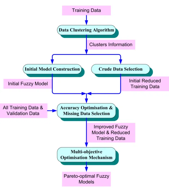
Figure 1 shows the flow chart of the proposed fuzzy modelling approach. This approach will be referred to throughout as the Hierarchical Fuzzy Modelling approach with a training Data Selection method and a Multi-objective Optimisation mechanism (HFM-DSMO). It can be divided into several parts and the execution steps can be described as follows:
1. Data clustering: A data clustering algorithm, such as the proposed new
version of the agglomerative complete-link clustering algorithm, is employed to process training data in order to obtain the information relating to clusters.
2. Initial model construction: The information about clusters is then used to
construct an initial fuzzy model.
3. Crude data selection: The clusters information is also used for a selection of
training data. Following this operation, an initial representative training data-set is obtained.
4. Accuracy optimisation and missing data selection: In this step, the initial
fuzzy model is briefly improved in terms of accuracy and a further representative training data set is selected. After this step, a relatively accurate fuzzy model is obtained and a complete reduced training data-set is formed.
5. Multi-objective optimisation: By using a multi-objective optimisation
algorithm, such as nMPSO [13, 14], the previous fuzzy model is further optimised according to the accuracy and interpretability objectives. Finally, a set of Pareto-optimal fuzzy models should be obtained.
<Figure 1>
2.2 Data clustering and initial fuzzy model construction
(groups) [30]. In fuzzy modelling, clustering techniques are widely used to generate the partitions of fuzzy sets automatically [31, 32].
In [11], a new hierarchical clustering algorithm, which is an improved agglomerative complete-link clustering algorithm, was designed to reduce the computation complexity and improve the efficiency. The algorithm has been shown to perform better than other well-known clustering algorithms, such as the fuzzy c-means (FCM) clustering algorithm [12], in initial fuzzy model generation.
By using the clustering algorithm, a predefined number of clusters can be obtained from the training data. The information that these clusters will provide is then used to construct an initial fuzzy model. In this modelling approach, one cluster corresponds directly to one fuzzy rule; the centres of membership functions are defined using the information of their corresponding clusters’ centre positions; other parameters relating to the membership functions are defined under the principle that one membership function must cover all the training data, which are included in its corresponding cluster. More details relating to this issue can be obtained from [11].
2.3 Training data selection
It is well-known that more training data will not necessarily lead to a better performance for data-driven models. Sometimes, one can identify a scenario where the training data are abundant and are concentrated in a small area of the input/output space. In this situation, if all the data are used in the training phase, then the areas with high data densities will be trained well and the areas with low data densities will be trained less so. It means that the extracted model will be accurate in some areas but not that so accurate in others.
To balance the training performance in different areas, one needs to reduce the training data in the areas with high data densities and some of the most representative data should be held and used in the later training phase. Obviously, another important advantage of the data selection mechanism is that it will save effort and time for training, since the data selection will reduce the size of the training data set.
For selecting the representative data that include all the important information of the original data set, the clustering technique may prove helpful. In data clustering, all the data are classified into several clusters with different features. In other words, the data in different clusters contain different information. Thus, the representative data should be selected from each cluster. To balance the influence of different clusters, the number of the selected data from each cluster should be approximately equal. For every cluster, the data with a minimal or maximal value in each dimension are very important. They provide one with the information of the cluster boundaries. The
generated model using this type of data can avoid the problem associated with generalisation. Therefore, these data should be included in the selected training data set.
In the previous initial fuzzy model extraction approach, the hierarchical clustering algorithm has been employed. The clustering result can be directly applied to select the training data. In summary, this selection method can be described as follows: For every cluster, the data including the minimal or maximal value in each input or output dimension are selected as the training data. If the number of the data which include the minimal or maximal value in one particular dimension is more than one, then only one data point (vector) will be randomly chosen and kept in the training data set. As a result, if the number of clusters is Nc and the dimension of the problem is D+1 (D
-input and 1-output), then the number of the selected training data will be less than 2×Nc×(D+1). This method can be qualified as a ‘crude data selection’.
The above training data selection method is able to find a set of training data with some representative features, but it may still miss some important data. First, if more than one datum includes the minimal or maximal value in one specific input or output dimension, some data will be abandoned. The abandoned data may however contain some important information. Second, the data located inside the clusters, which do not have any minimal or maximal value, are also likely to contain some useful information for modelling.
Compared with the data that have already been selected, the missing data representative must possess some different features. Thus, the prediction model, which is trained based on the data that have already been selected, must be inaccurate as far as the missing data are concerned. As a result, the following method is proposed which is used to detect the missing representative data to be added to the training data set:
1. Train the initial fuzzy model using the data selected by the ‘crude data selection’ method. This model does not need to be well optimised.
2. Calculate the output prediction of all the available training data using the trained model. Find a set of data with the biggest differences between the predicted output value and the true output value.
3. The data found in Step 2 are added to the training data set and the new training data set is used to improve the existing fuzzy model.
It should be noted that the above missing data selection procedure may need to be repeated several times to ensure that all the representative data are included in the final selected training data set.
By combining the initially selected training data and the subsequently detected training data, one can obtain the final training data, which are the representatives of
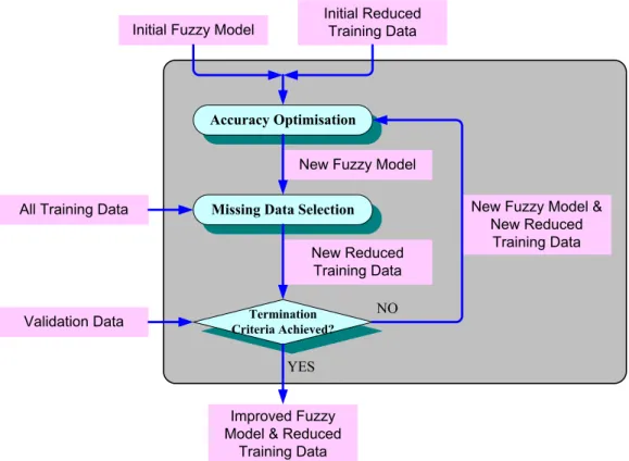
all the training data which can then be used in the next model improvement stage. Figure 2 shows the flow chart of the joint mechanism for accuracy optimisation and missing data detection. Normally, the termination criterion for this mechanism is designed so that the loop iteration achieves a predefined number.
<Figure 2>
2.4 Multi-objective optimisation of accuracy and interpretability
The improvement of interpretability of fuzzy systems is tantamount to reducing the number of fuzzy rules, reducing the length of fuzzy rules, reducing the number of fuzzy sets, and adjusting these sets to be evenly distributed along the universes of discourse. These tasks can be achieved using the following four-step operation (Section 2.4.1 – 2.4.4).
2.4.1 Removing redundant fuzzy rules
This operation can reduce the number of fuzzy rules. Concomitantly, some fuzzy sets, which are only involved in these redundant rules, may also be removed. To evaluate whether a fuzzy rule is redundant or not, two evaluation measures are used, namely
confidence and support [33]. In [33], the confidence measure is introduced as follows:
N i i N i i B i y B conf 1 1 ) ( ) ( ) ( ) ( x x A A A , (1)where μA(xi) is the compatibility grade of the input vector xi with the antecedent part
A = [A1, A2, …, AD]T of the fuzzy rule R, and μB(yi) is the compatibility grade of the
output value yi with the consequent part B of R. μA(xi) is usually defined by the
minimum operator or the product operator [33]. Such as:
( ), ( ), , ( )
min ) ( 1 1 2 2 i D A i A i A i x x D x A x or (2) ) ( ) ( ) ( ) ( 1 1 2 2 i D A i A i A i x x D x A x , (3)where μAj(xji) is the membership function of the antecedent fuzzy set Aj. On the other
hand, the support of a fuzzy rule A→ Bis defined as follows [33]:
N y B supp N i i B i
1 ) ( ) ( ) ( x A A . (4)In this work, the product of support and confidence is used as the criterion for the fuzzy rule selection. A threshold Th1 for this rule selection is also defined. If the product criterion of one rule is smaller than the threshold Th1, then this fuzzy rule is deemed redundant, and as a consequence the fuzzy rule and the fuzzy sets that are
only included by this redundant rule are removed.
2.4.2 Merging similar fuzzy rules
This operation can reduce the number of fuzzy rules. At the same time, the fuzzy sets involved within similar rules are also merged.To decide whether two fuzzy rules are similar enough for combination or not, one only needs to evaluate the similarity of the antecedent parts of the rules. Two fuzzy rules with very similar antecedents but different consequents usually indicate that these two rules conflict with each other. Therefore, we should either merge these rules into one new rule or delete one of them. To calculate the degree of similarity for the antecedents of two fuzzy rules, the similarity of every fuzzy set pair should be checked. For the kth fuzzy rule Rk, the
corresponding preconditions are A1k, A2k, …, ADk. Similarly, the corresponding
antecedents of the lth rule Rl are A1l, A2l, …, ADl. Thus, the similarity measure can be
characterised as follows [20]:
D m l m k m l k R R R S A A S 1 ) , ( ) , ( , (5)where S(Amk, Aml) is the similarity of two fuzzy sets Amk and Aml and it is defined in
Section 2.4.4.
Once SR(Rk, Rl) reaches a threshold Th2, then these two fuzzy rules as well as the fuzzy set pairs of these two rules are considered to be similar. The two fuzzy rules are then merged into a new rule Rnew. The new antecedents and consequent of Rnew are
obtained by merging the corresponding fuzzy sets (see Section 2.4.4).
2.4.3 Removing redundant fuzzy sets
This operation can reduce the number of fuzzy sets by removing the ones that cover others. In addition, this operation can also shorten the length of fuzzy rules because some of their premises, which include redundant fuzzy sets, should also be removed from the fuzzy rules simultaneously.
In this method, the similarity for each fuzzy set An to the universal set U (μU(x) = 1) is
calculated. If the similarity value is greater than a threshold value Th3, then this fuzzy set is counted as a redundant fuzzy set. As a result, the associated fuzzy set should be removed. If Gaussian membership functions are involved, then the similarity of one fuzzy set to the universal set can be represented using the parameter σn.
2.4.4 Merging similar fuzzy sets
as not to overlap. For an evaluation purpose, some fuzzy similarity measures have already been introduced in the past [34], one of which is as follows:
) , ( 1 1 ) , ( 2 1 2 1 A A d A A S , (6) where d(A1, A2) is the distance between two fuzzy sets A1 and A2.
If Gaussian membership functions are employed, then the distance between two fuzzy sets can be approximated using the following simple expression [35]:
2 2 1 2 2 1 2 1, ) ( ) ( ) (A A c c d . (7)
A threshold Th4 for merging similar fuzzy sets is then defined, where Th4∈ (0, 1]. If
S(A1, A2) > Th4, i.e., the fuzzy sets A1 and A2 are highly overlapping, then these two fuzzy sets should be merged into one new fuzzy set Anew, where cnew = (c1 + c2) / 2 and
σnew = (σ1 + σ2) / 2. Because the fuzzy sets in the antecedent part and those in the consequent part have a different influence on the performance of a fuzzy model, different thresholds should be separately set.
2.4.5 The proposed multi-objective optimisation mechanism
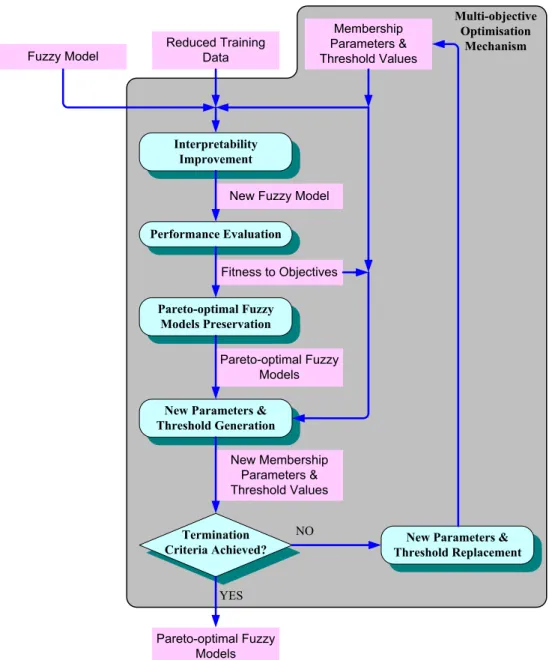
Based on the advised four-step interpretability improvement operation, a multi-objective optimisation mechanism, which is intended to optimise both the accuracy and the interpretability of fuzzy systems, is developed. Specifically, a multi-objective optimisation algorithm is employed to optimise the parameters of the membership functions of fuzzy sets, as well as optimise the rule base by finding the optimal thresholds for interpretability improvement operation. Figure 3 outlines the procedure behind the proposed mechanism. It works according to the following steps:
1. Initial threshold values generation: Randomly generate the values of
thresholds within predefined bounds.
2. Interpretability improvement: Based on the reduced training data, improve
the previous fuzzy model in interpretability using the proposed 4-step improvement operation. In this step, the input rule-base is fixed and remains as such while the parameters of the membership functions and the thresholds vary after each loop. Following this step, a new fuzzy model is elicited.
3. Performance evaluation: The new fuzzy model is evaluated using designed
fitness functions (objective functions).
4. Pareto-optimal fuzzy models preservation: Compare the fitness of every
generated model; preserve the adequate Pareto-optimal models via the archive mechanism in nMPSO [13].
5. New parameters and thresholds generation: This task is accomplished by
the nMPSO algorithm based on some particular principles, which are related to the fitness values and the location of individual solutions.
6. Termination estimation: If the termination criteria are achieved, then stop the mechanism and return the final Pareto-optimal fuzzy models; otherwise, replace the old membership function’s parameters and threshold values with new ones and go back to Step 2.
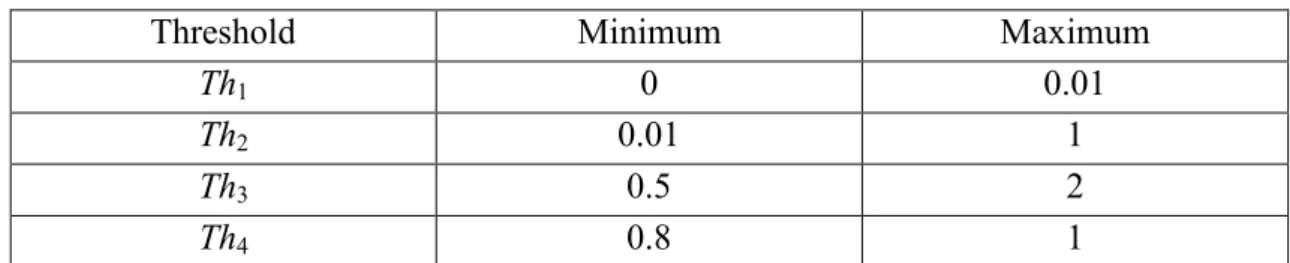
Normally, the termination criteria are designed so that the number of function evaluations achieves a predefined value. It should been noted that the structure of a fuzzy model is not directly coded into the optimisation procedure, but is rather varied and optimised via controlling the thresholds. Generally, it is recommended that the thresholds should be located in the ranges shown in Table 1.
<Figure 3> <Table 1>
The accuracy of a fuzzy model can be evaluated using the Root Mean Square Error (RMSE) index, which is described as follows:
N y y RMSE N l p l m l
1 2 , (8)where ylm is the measured output data and ylp is the predicted output data, l = 1, 2, …, N; N is the total number of data. The interpretability of a fuzzy model is affected by the number of fuzzy rules (Nrule), the number of fuzzy sets (Nset) and the total length of fuzzy rules (Lrule).
To normalise these two objectives and make them similar and comparable in scale, they are formulated as follows:
Objective 1: I RMSE RMSE ; Objective 2: I I I Lrule Lrule Nset Nset Nrule Nrule ; (9)
where RMSEI is the root mean square error of the fuzzy model that is not optimised
using the multi-objective optimisation mechanism; NruleI, NsetI and LruleI represent
the number of fuzzy rules, the number of fuzzy sets and the total rule length of this fuzzy model, respectively.
In this mechanism, an improved version of PSO is employed. PSO is a powerful evolutionary computation technique that was originally introduced by Kennedy and Eberhart [36]. It was developed via the simulation of a simplified animal social behaviour of birds flocking and fish schooling. As a numerical optimisation algorithm, PSO is more suitable than the heuristic algorithms that are mainly designed for combinatorial optimisation problems, such as tabu search [37] and ant colony optimisation [38]. Compared with other numerical optimisation algorithms, such as
genetic algorithm [39] and artificial immune systems [40], PSO is easy to implement and is able to quickly converge to a reasonably good solution [21].
In the previously reported work [13], an alternative structure for PSO, named ‘nPSO’, was introduced. In nPSO, a ‘momentum term’ was proposed to replace the original inertia term of the standard PSO, which can help to avoid premature convergence and encourage the particles to jump out of any local optimum. To provide the particles of nPSO with more adaptability, a separate momentum weight was assigned to each particle as it dynamically adjusts itself according to the particle’s own search experience. In the later paper [14], the nPSO algorithm was further improved, whereby the population size of this algorithm can also be dynamically varied according to the algorithm’s search performance in the optimisation process. The modified algorithm was then extended to a multi-objective optimisation case as ‘nMPSO’. These proposed algorithms have been compared with some salient single-objective and multi-single-objective evolutionary algorithms using a large set of difficult benchmark optimisation problems. The results showed that the proposed algorithms outperform the other algorithms in most cases.
2.5 Confidence band analysis
Once the final fuzzy models have been elicited, one wishes to know how confident one can be of a particular output a prediction. Normally, the standard deviation of the prediction errors of all the training data is computed in order to represent the confidence band. But the standard deviation can only inform on a generalised view about the model. It cannot provide particular guidance for one specific prediction. For example, for different predictions given by a developed model, the tolerance should be different, while the standard deviation is only a fixed value, which shows the general confidence degree relating to the model.
In this work, a confidence band named α%-range confidence band is designed. It is calculated as follows:
1. When given a prediction value yp, define a prediction scope S where the lower bound is yp-0.005×α×Lp and the upper bound is yp+0.005×α×Lp, with Lp being
the total range of the prediction values and it equals to the maximal prediction value minus the minimal prediction value.
2. From all the training data, find the ones pi with their prediction output values
yip including in the scope S, which is yip S, where i = 1, 2, …, Ns and Nsis
the number of training data pi.
3. The α%-range confidence band CB is defined using the standard deviation of the prediction errors of the training data pi:
s N j j N error error Error Std CB s 2 1( ) ) (
, (10)where Error = {error1, error2, …, errorNs}; errorj = yjp - yjm; yjm are the
measured output values of pi; i = 1, 2, …, Ns.
For an obtained model, it is not realistic to calculate the α%-range confidence band for every possible prediction. Generally, some averagely distributed prediction values are selected to provide some confidence bands which will be viewed as the representatives of all the possible prediction values.
3. Experimental studies
In order to validate the effectiveness of the proposed modelling strategy HFM-DSMO, the associated approach was applied to the modelling of two benchmark problems, one is a problem of static nonlinear system approximation and the other is a dynamical system identification problem. Furthermore, HFM-DSMO was applied to the modelling of mechanical properties of alloy steels using a large amount of high-dimensional, real industrial data.
3.1 The nonlinear function approximation
In this experiment, the proposed fuzzy modelling approach was used to approximate the following two-input-single-output nonlinear static system, which is introduced in [41]: 2 5 . 1 2 2 1 ) 1 ( x x y , 1x1,x2 5. (11)
In order to establish a quantitative comparison with the results obtained in other papers, the training data set was selected as being the same as the one described in [41], which consists of 50 data points. Furthermore, another 50 randomly generated data points were used for model testing.
In this case, the initial fuzzy model was obtained using 8 clusters, resulting in a model with 8 rules and 24 fuzzy sets. For the optimisation algorithm nPSO and nMPSO [13], the population size was set to be 10; the acceleration coefficients c1 and c2 were set to 1.5; the scaling parameters m1 and m2 were set to 0.5 and 2 respectively; ε = 10-10; the position parameter posid was updated using both the one-directional refresh
mechanism (with the 70% probability of usage) and the multiple-directional refresh mechanism (with the 30% probability of usage) [13]; for nMPSO, the frequency of the weight changing H = 2000; the maximum number of function evaluation for nPSO and nMPSO were both set to 20,000. This parameters configuration was inspired from suggestions included in [11]. The data selection mechanism was not applied since the
training data are not considered to be redundant in this case.
The experiment was carried over for 20 runs. One set of results out of the 20 runs is randomly selected and shown in the following figures. Figure 4 shows their performances with respect to various indices, including the root mean square error, the number of fuzzy rules, the number of fuzzy sets and the length of the fuzzy rules. Figure 5 shows the prediction performance of the initial as well as the three selected fuzzy models, which include 8, 6 and 4 rules respectively. Figure 6 illustrates the distribution of their membership functions relating to two inputs (x1 and x2). It can be seen that, for these optimised models, more rules and more parameters will bring more accuracy while the models with fewer rules and parameters are simpler in structure and easier to understand.
<Figure 4> <Figure 5> <Figure 6>
To provide more details about these Pareto-optimal models, Figure 7 shows the rule-base relating to the optimised system, which is the one associated with 8 rules, its other information being included in Figures 5(b) and 6(b). For this fuzzy model, the linguistic hedges approach [42] can be employed to derive the corresponding approximate linguistic rules [7, 41] as follows:
R1: IF x2 is small, THEN y is medium large.
R2: IF x1 is medium small AND x2 is medium large, THEN y is medium.
R3: IF x1 is more or less medium large AND x2 is medium small, THEN y is
medium small.
R4: IF x1 is small, THEN y is large.
R5: IF x1 is medium AND x2 is medium large, THEN y is small.
R6: IF x1 is very medium AND x2 is medium, THEN y is medium small. R7: IF x2 is large, THEN y is small.
R8: IF x1 is large AND x2 is medium, THEN y is small.
By inspecting these linguistic rules, one can understand more about the system’s behaviour.
<Figure 7>
Figure 8 shows the three-dimensional input-output surfaces of the actual system and the optimised 8-rule fuzzy system. The 5%-range confidence band of this 8-rule fuzzy model is displayed in Figure 9. From this figure, one can infer more details of how confident one can be about a prediction. For instance, when a prediction is 4.6, its confidence band is relatively large, which means this prediction is not very reliable compared with most of the other predictions.
<Figure 8> <Figure 9>
Table 2 describes the experimental results compared with those published via other research studies. Three groups of models out of all the Pareto-optimal models in 20 runs, which include 8, 6 and 4 rules respectively, are chosen as the representatives and are listed in this table. It can be seen that HFM-DSMO performs better than the method, whose strategy is based on linguistic fuzzy systems [41]; for the method based on singleton fuzzy systems [1], it needs more fuzzy rules to reach the same accuracy level as that of HFM-DSMO.
<Table 2>
3.2 The identification of a dynamic system
In this problem, the modelling target is a nonlinear second-order plant, which has been studied in [43-46],
( 1), ( 2)
( ) ) (k g y k y k u k y , (12) where
) 2 ( ) 1 ( 1 5 . 0 ) 1 ( ) 2 ( ) 1 ( ) 2 ( ), 1 ( 2 2 k y k y k y k y k y k y k y g . (13)where y() is the output of the system; g() is a nonlinear component; u() is the input signal; k is the index of the input signals.
The output of this system depends on both its past states and the current input. The modelling purpose is to approximate the nonlinear component g(y(k – 1), y(k – 2)). Following the experimental settings in [46], 400 simulated data samples were generated from the plant model (12). With the starting equilibrium state (0, 0), the first 200 samples of training data were obtained by using a random input signal u(k) that is uniformly distributed in the interval [-1.5, 1.5] and the rest 200 samples of testing data were obtained by using a sinusoidal input signal u(k) = sin(2πk/25).
In this case, the initial fuzzy model was also obtained with 8 clusters; the parameters of the optimisation paradigms were set the same as those in Section 3.1; the data selection mechanism was also not used in this case, since the training data are not redundant.
This experiment was repeated 20 times. One set of models out of the 20 runs is randomly selected and shown in the following figures. Figure 10 demonstrates the trade-offs among the multiple objectives and criteria within 13 non-dominated fuzzy
system solutions.
<Figure 10>
To provide more details about these non-dominated models, the fuzzy rule-base of an optimised model, which includes 6 rules, is shown in Figure 11. For this fuzzy model, the following approximate linguistic rules can be derived by using the linguistic hedges approach [7, 41, 42]:
R1: IF y(k – 1) is small AND y(k – 2) is medium large, THEN g(k) is large. R2: IF y(k – 1) is large AND y(k – 2) is medium large, THEN g(k) is large. R3: IF y(k – 1) is small AND y(k – 2) is medium small, THEN g(k) is small. R4: IF y(k – 1) is medium AND y(k – 2) is more or lessmedium small, THEN
g(k) is medium.
R5: IF y(k – 1) is large AND y(k – 2) is medium small, THEN g(k) is medium
small.
R6: IF y(k – 1) is medium AND y(k – 2) is medium large, THEN g(k) is
medium.
By inspecting these linguistic rules, one can obtain more knowledge relating to the system’s behaviour.
<Figure 11>
Figure 12 shows the three-dimensional response surfaces of the actual system and the optimised 6-rule fuzzy system. It can be observed that these two surfaces are perfectly matched. The 6-rule model’s 5%-range confidence band is shown in Figures 13.
<Figure 12> <Figure 13>
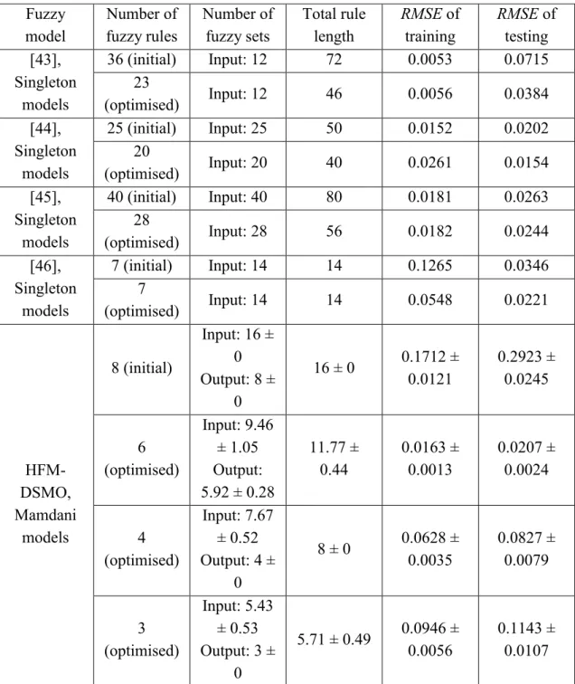
Table 3 compares the experimental results with some other studies previously reported in the literature [43-46]. Three groups of models out of all the Pareto-optimal models in 20 runs, which include 6, 4 and 3 rules respectively, together with the initial generated models are listed in this table. It can be seen that HFM-DSMO is able to produce more compact and simpler models compared to the other methods, since the modelling strategies reported in [43-45] needed more fuzzy rules and fuzzy sets to achieve the same accuracy level as that of HFM-DSMO. In other words, this proposed approach seems to strike a good balance between numerical accuracy and model simplicity, compared to the above mentioned fuzzy modelling methods.
<Table 3>
In material engineering, specialist heat treatments consist of two main stages: hardening and tempering, are used to develop the required mechanical properties in a range of alloy steels [47]. It is not possible to accurately describe the process behaviour using mathematical models alone due to the complexity of the underlying physical mechanisms. In this work, several most important mechanical properties of heat-treated alloy steels are studied, including UTS, elongation and Charpy impact energy. The UTS represents a measure of the maximum load that a material can withstand. The elongation is a measure of ductility, which is usually expressed as a percentage change in the gauge length or diameter of the specimen after fracture [48]. Both the UTS and the elongation are obtained via an engineering tension test. On the other hand, a Charpy impact test is used as the indicator of toughness. It measures the energy (Charpy impact energy) necessary to fracture a standard Charpy V-notch bar specimen, by an impulse load [47].
All the data related to mechanical properties, which are used in this paper, are provided by Tata Corus (UK). They include no less than fifteen input variables and are considered as high-dimensional problems for modelling purposes. The UTS data include 15 inputs, which consist of the weight percentages for the chemical composites, namely carbon (C), silica (Si), manganese (Mn), sulphur (S), chromium (Cr), molybdenum (Mo), nickel (Ni), aluminium (Al) and vanadium (V), the test depth, the bar size, the treatment site, the quenching medium, as well as the hardening and tempering temperatures. In the elongation case, there are totally 16 inputs, which include all the inputs of the UTS case and another one, the elongation gauge length. The Charpy impact energy data also have 16 inputs variables, including the ones of the UTS data as well as the impact test temperature.
Moreover, these modelling problems are associated with a large number of industrial data, including 3760 UTS data, 3804 elongation data and 1661 Charpy impact energy data. In the following sections, for one specific experiment, 75% of the data are used for training, 10% of the data are used for validation and the remaining 15% are used for final testing.
3.3.1 The prediction of UTS
In this experiment, the initial number of clusters was set to 15, which means that the initial fuzzy model was generated using 15 rules. For the optimisation algorithms nPSO and nMPSO, the parameter settings were the same as those in Section 3.1, except that the maximum numbers of function evaluation were both set to 50,000. After the operation of the training data selection mechanism, 440 data points out of 2820 data points (all the training data) were selected and worked as the representatives of all the training data.
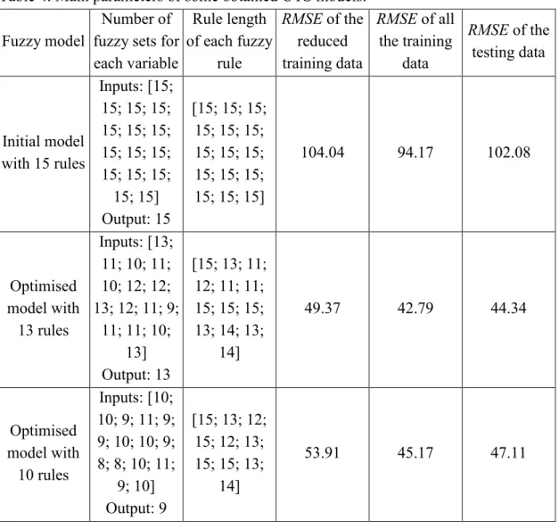
The experiment was run 20 times. One set of models out of the 20 runs is randomly chosen and shown in the following paragraphs. Figure 14 demonstrates the trade-offs among the multiple objectives and criteria, including the RMSE, the number of fuzzy rules, the number of fuzzy sets and the total length of fuzzy rules, within these Pareto-optimal fuzzy models. Table 4 includes the main parameters of the initial model and the two optimised models, which are selected from all the Pareto-optimal models with 13 and 10 rules respectively.
<Figure 14> <Table 4>
Figure 15 shows the prediction performance of these models. It can also be seen that the selected training data work well as the representatives of all the training data. By using these reduced data instead of all the training data, much computational time and user effort can be saved.
<Figure 15>
For more details about these Pareto-optimal UTS models, Figure 16 shows two rules (the 3th rule and the 8th rule) out of the rule-base of the optimised 10-rule model. For these fuzzy rules, they can be rewritten as the following approximate linguistic rules using the linguistic hedges approach:
R3: IF Test Depth is small AND Size is more or less medium AND Site Number is more or less medium AND Si is medium AND Mn is small
AND S is small AND Cr is medium small AND Mo is medium small
AND Ni is more or less medium AND V is very small AND Tempering Temperature is large, THEN UTS is medium small.
R8: IF Test Depth is more or less medium small AND Size is small AND Site Number is more or less large AND C is medium AND Si is more or
less medium AND Mn is small AND S is medium small AND Cr is
large AND Mo is more or less medium small AND Al is very small
AND V is more or less small AND Hardening Temperature is more or
less not large AND Cooling Medium Number is more or less medium
AND Tempering Temperatures is medium, THEN UTS is large.
It is clear that such linguistic fuzzy rules allow for a better insight into the heat-treated alloy steels process.
<Figure 16>
To verify the physical interpretation of the obtained models, Figure 17 shows the three-dimensional response surfaces of the 10-rule UTS model. These surfaces are
achieved by plotting two varying input variables against the output while keeping other input variables constant. The constant variables are set to the average values of the dominant steel grade, which is the 1%CrMo steel grade [47]. These plots in Figure 17 are consistent with those variable effect plots in [47], which have been verified to follow the expected behaviour as predicted by theory or by expert knowledge. This 10-rule model’s 5%-range confidence band is shown in Figure 18. From this figure, one can see that, for a prediction around 1700, it is more robust and reliable, when compared with a prediction around 1000.
<Figure 17> <Figure 18>
3.3.2 The prediction of elongation
In this case, the configuration of all the parameters was set the same as those used in Section 3.3.1. After the data selection mechanism, 500 representative data points out of 2853 data points were selected and then used in the following training process. The experiment was run 20 times. One set of models out of the 20 runs is randomly selected and shown as follows:
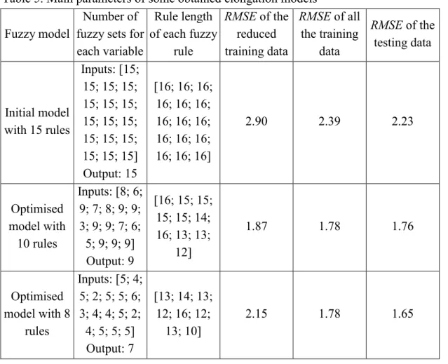
Figure 19 shows the trade-offs among the multiple criteria within these non-dominated fuzzy models. Table 5 describes the main parameters of the initial elongation model and two optimised elongation models with 10 and 8 rules respectively, and Figure 20 shows the prediction performance of these models.
<Figure 19> <Table 5> <Figure 20>
The response surfaces of the 10-rule elongation model are shown in Figure 21, where the constant variables are set to be the average values of the 1%CrMo steel grade. These surfaces reveal a consistent match with the variable effect plots in [47], and this means the constructed models follow the expected behaviour as predicted by theory or by expert knowledge.
<Figure 21>
3.3.3 The prediction of Charpy impact energy
In this example, the configuration of all the parameters was set the same as those in Section 3.3.1. Following the data selection exercise in Section 2.3, 455 data points out of 1246 data points were selected. The experiment was run 20 times. One set of
models out of these 20 runs is randomly selected and shown as follows:
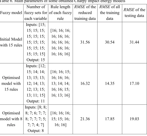
Figure 22 shows the trade-offs among the multiple criteria within these non-dominated fuzzy solutions. Table 6 shows the main parameters of the initial impact energy model and two optimised impact energy models with 15 and 8 rules respectively. Figure 23 shows the prediction performance of these models.
<Figure 22> <Table 6> <Figure 23>
Figure 24 shows the three-dimensional response surfaces of the 15-rule impact energy model. For this case, the constant variables are set to the average values of the 1%CrMo steel grade. This figure reveals a consistent match with the variable effect plots in [47], which have been verified to follow the theoretical or expert knowledge. It is also worth noting that the proposed modelling approach has a good nonlinear mapping and generalisation ability, which is evidenced by the smooth input-output response surfaces in Figures 8(b), 12(b), 17, 21 and 24.
<Figure 24>
4 Conclusions
In this paper, a framework for data-driven fuzzy modelling, named HFM-DSMO, is proposed. It allows to construct Mamdani fuzzy models considering both the accuracy (precision) and the transparency (interpretability) attributes. Within this methodology, a fast hierarchical clustering algorithm is employed for the initial fuzzy model generation, which can reduce the computational complexity compared with its former version. Second, a training data selection mechanism is proposed for choosing most appropriate and efficient training data so as to save effort and time in training. Third, a high-performance multi-objective optimisation mechanism, which is based on the previously developed efficient optimisation algorithm nMPSO, is developed in order to optimise both the parameters and the structure of fuzzy systems in different accuracy and interpretability levels. Finally, a new analytical method is proposed for deriving the confidence bands relating to the final elicited models.
The experimental validation was then carried out based on two benchmark problems, a static nonlinear system approximation problem and a dynamical system identification problem. The experimental results have revealed that, HFM-DSMO works effectively in eliciting accurate and interpretable models; compared to other modelling methods, HFM-DSMO is able to produce more compact and simpler models.
Furthermore, the proposed modelling approach was successfully applied within the context of manufacturing of heat-treated alloy steels, which aims to predict the mechanical properties for heat-treated alloy steels by correlating them with the heat treatment process conditions as well as the weight percentages of the chemical composites using complex, high-dimensional industrial data. The physical interpretation of the obtained models has been shown to be consistent with the expected behaviour as predicted by theory or by expert knowledge. In addition to the above, it is worth noting that the fuzzy models constructed using HFM-DSMO has a good generalisation ability, which is evidenced by the smooth input-output response surfaces obtained using the elicited models.
Acknowledgements
The authors wish to thank the anonymous reviewers for their comments which helped to improve the quality of this paper. They also wish to acknowledge financial support for this work from The European Union under Framework-6 and the UK-EPSRC under Grant Reference Number: EP/E063497/1.
References:
[1] I. Rojas, H. Pomares, J. Ortega, A. Prieto, Self-organized fuzzy system generation from training examples, IEEE Transactions on Fuzzy Systems 8 (1) (2000), pp. 23–36.
[2] F.B. Pickering, Physical Metallurgy and the Design of Steels, Applied Science, London, 1978.
[3] C.K. Kwong, Y. Chen, K.Y. Chan, H. Wong, Hybrid fuzzy least-squares regression approach to modeling manufacturing processes, IEEE Transactions on
Fuzzy Systems, 16 (3) (2008), pp. 644-651.
[4] K.Y. Chan, C.K. Kwong, Y.C. Tsim, A genetic programming based fuzzy regression approach to modeling manufacturing processes, International Journal
of Production Research, 48 (7) (2009), pp. 1967-1982.
[5] C.L.P. Chen, C. Yang, S.R. LeClair, Materials structure-property prediction using a self-architecting neural network, Journal of Alloys Compounds 279 (1) (1998), pp. 30–38.
[6] B.R. Bakshi, R. Chatterjee, Unification of neural and statistical methods as applied to materials structure-property mapping, Journal of Alloys Compounds 279 (1) (1998), pp. 39–46.
[7] M.-Y. Chen, D.A. Linkens, A systematic neuro-fuzzy modeling framework with application to material property prediction, IEEE Transactions on Systems, Man,
and Cybernetics - Part B: Cybernetics31 (5) (2001), pp. 781–790.
knowledge-based neural-fuzzy modelling, ISIJ International 46 (4) (2006), pp. 586–590.
[9] E.H. Mamdani, S. Assilian, An experiment in linguistic synthesis with a fuzzy logic controller, International Journal of Man-Machine Studies7 (1) (1975), pp. 1–13.
[10] T. Takagi, M. Sugeno, Fuzzy identification of systems and its applications to modeling and control, IEEE Transaction Systems, Man and Cybernetics 15 (1) (1985), pp. 116–132.
[11] Q. Zhang, Nature-Inspired Multi-Objective Optimisation and Transparent Knowledge Discovery via Hierarchical Fuzzy Modelling. PhD Thesis, The Department of Automatic Control and Systems Engineering, The University of Sheffield, UK, 2008.
[12] J.C. Bezdek, Pattern Recognition with Fuzzy Objective Function Algoritms, Plenum Press, New York, 1981.
[13] Q. Zhang, M. Mahfouf, A new structure for particle swarm optimization (nPSO) applicable to single objective and multiobjective problems, Proceedings of the 3rd
International IEEE Conference on Intelligent Systems, 2006, pp. 176–181.
[14] Q. Zhang, M. Mahfouf, A modified PSO with a dynamically varying population and its application to the multi-objective optimal design of alloy steels,
Proceedings of the 2009 IEEE Congress on Evolutionary Computation, 2009, pp.
3241–3248.
[15] L.A. Zadeh, Fuzzy sets, Information and Control8 (3) (1965), pp. 338–353. [16] L.A. Zadeh, Outline of a new approach to the analysis of complex systems and
decision processes, IEEE Transactions on Systems, Man, and Cybernetics 3
(1973), pp. 28–44.
[17] L.-X. Wang, J. M. Mendel, Fuzzy basis functions, universal approximation, and orthogonal least-squares learning, IEEE Transactions on Neural Networks 3 (5) (1992), pp. 807-814.
[18] J.-S.R. Jang, C.-T. Sun, E. Mizutani, Neuro-Fuzzy and Soft Computing, Prentice-Hall, Englewood Cliffs, NJ, 1997.
[19] O. Cordon, F. Herrera, F. Hoffmann, L. Magdalena, Genetic Fuzzy Systems – Evolutionary Tuning and Learning of Fuzzy Knowledge Bases, World Scientific, Singapore, 2001.
[20] Y. Jin, W. von Seelen, B. Sendhoff, On generating FC3 fuzzy rule systems from data using evolution strategies, IEEE Transactions on Systems, Man, and
Cybernetics - Part B: Cybernetics29 (6) (1999), pp. 829–845.
[21] R.C. Eberhart, Y. Shi, J. Kennedy, Swarm Intelligence, Morgan Kaufmann, San Mateo, CA, 2001.
[22] H. Ishibuchi, Y. Nojima, Analysis of interpretability-accuracy tradeoff of fuzzy systems by multiobjective fuzzy genetics-based machine learning, International
Journal of Approximate Reasoning44 (1) (2007), pp. 4–31.
multi-objective evolutionary approach to the identification of Mamdani fuzzy systems,
Soft Computing11 (11) (2007), pp. 1013–1031.
[24] M.J. Gacto, R. Alcala, F. Herrera, Adaptation and application of multi-objective evolutionary algorithms for rule reduction and parameter tuning of fuzzy rule-based systems, Soft Computing13 (5) (2009), pp. 419–436.
[25] R. Alcala, P. Ducange, F. Herrera, B. Lazzerini, F. Marcelloni, A multiobjective evolutionary approach to concurrently learn rule and data bases of linguistic fuzzy-rule-based systems, IEEE Transactions on Fuzzy Systems17 (5) (2009), pp. 1106–1122.
[26] T.A. Johansen, R. Babuska, Multiobjective identification of takagi-sugeno fuzzy models, IEEE Transactions on Fuzzy Systems11 (6) (2003), pp. 847–860.
[27] H. Wang, S. Kwong, Y. Jin, W. Wei, K.F. Man, Agent-based evolutionary approach for interpretable rule-based knowledge extraction, IEEE Transactions on
Systems, Man, and Cybernetics - Part C: Applications and Reviews, 35 (2) (2005),
pp. 143–155.
[28] H. Wang, S. Kwong, Y. Jin, W. Wei, K.F. Man, Multi-objective hierarchical genetic algorithm for interpretable fuzzy rule-based knowledge extraction, Fuzzy Sets and Systems149 (2005), pp. 149–186.
[29] A.F. Gomez-Skarmeta, F. Jimenez, G. Sanchez, Improving interpretability in approximative fuzzy models via multiobjective evolutionary algorithms,
International Journal of Intelligent Systems22 (9) (2007), pp. 943–969.
[30] A.K. Jain, M.N. Murty, P.J. Flynn, Data clustering: a review, ACM Computing
Surveys31 (3) (1999), pp. 264–323.
[31] Y. Yoshinari, W. Pedrycz, K. Hirota, Construction of fuzzy models through clustering techniques, Fuzzy Sets and Systems, 54 (1993), pp. 157-165.
[32] M. Delgado, A.F. Gomez-Skarmeta, A. Vila, On the use of hierarchical clustering in fuzzy modeling, International Journal of Approximate Reasoning, 14
(1996), pp. 237-257.
[33] H. Ishibuchi, T. Yamamoto, T. Nakashima, Fuzzy data mining: effect of fuzzy discretization, Proceedings of the First IEEE International Conference on Data
Mining, 2001, pp. 241–248.
[34] M. Setnes, R. Babuska, B. Verbruggen, Rule-based modeling: precision and transparency, IEEE Transactions on Systems, Man, and Cybernetics - Part C 28
(1) (1998), pp. 165–169.
[35] Y. Jin, Fuzzy modeling of high-dimensional systems: complexity reduction and interpretability improvement, IEEE Transactions on Fuzzy Systems 8 (2) (2000), pp. 212–221.
[36] J. Kennedy, R.C. Eberhart, Particle swarm optimization, Proceedings of the
IEEE International Conference On Neural Networks, 1995, pp. 1942–1948.
[37] F. Glover, M. Laguna, Tabu Search. Kluwer, Norwell, MA, 1997. [38] M. Dorigo, T. Stutzle, Ant Colony Optimization, MIT Press, 2004.
Learning. Addison Wesley, Reading, MA, 1989.
[40] L.N. De Castro, J. Timmis, Artificial immune systems: a new computational intelligence approach, Springer, 2002.
[41] M. Sugeno, T. Yasukawa, A fuzzy-logic-based approach to qualitative modeling,
IEEE Transactions on Fuzzy Systems1 (1) (1993), pp. 7–31.
[42] L.A. Zadeh, A fuzzy-set-theoretic interpretation of linguistic hedges, Journal of
Cybernetics, 2 (1972), pp. 4-34.
[43] J. Yen, L. Wang, Application of statistical information criteria for optimal fuzzy model construction, IEEE Transactions on Fuzzy Systems 6 (3) (1998), pp. 362– 372.
[44] J. Yen, L. Wang, Simplifying fuzzy rule-based models using orthogonal transformation methods, IEEE Transactions on Systems, Man, and Cybernetics -
Part B: Cybernetics29 (1) (1999), pp. 13–24.
[45] L. Wang, J. Yen, Extracting fuzzy rules for system modeling using a hybrid of genetic algorithms and Kalman filter, Fuzzy Sets and Systems 101 (1999), pp. 353–362.
[46] M. Setnes, H. Roubos, GA-fuzzy modeling and classification: complexity and performance, IEEE Transactions on Fuzzy Systems8 (5) (2000), pp. 509–522. [47] J. Tenner, Optimisation of the Heat Treatment of Steel Using Neural Networks,
PhD Thesis, The Department of Automatic Control and Systems Engineering, The University of Sheffield, UK, 1999.
[48] G.E. Dieter, Mechanical metallurgy: SI metric edition, McGraw-Hill, London, 1988.
Tables:
Table 1. Recommended ranges for thresholds
Threshold Minimum Maximum
Th1 0 0.01
Th2 0.01 1
Th3 0.5 2
Th4 0.8 1
Table 2. The performance comparison of various models for the nonlinear function approximation problem. Fuzzy model Number of fuzzy rules Number of fuzzy sets Total rule length RMSE of training RMSE of testing [41], Mamdani models 6 (initial) Input: 12 Output: 6 12 0.5639 N/A 6 (optimised) Input: 12 Output: 6 12 0.2811 N/A [1], Singleton models
9 (case 1) Input: 6 18 0.5126 N/A
16 (case 2) Input: 8 32 0.1755 N/A
25 (case 3) Input: 10 50 0.0658 N/A
HFM-DSMO, Mamdani models 8 (initial) Input: 16 ± 0 Output: 8 ± 0 16 ± 0 0.3828 ± 0 0.4457 ± 0.1227 8 (optimised) Input: 13.63 ± 1.41 Output: 7.88 ± 0.35 15.25 ± 1.04 0.0262 ± 0.0029 0.0801 ± 0.0140 6 (optimised) Input: 10.67 ± 0.82 Output: 5.95 ± 0.23 11.86 ± 0.38 0.0582 ± 0.0038 0.1146 ± 0.0201 4 (optimised) Input: 6.85 ± 0.69 Output: 4.00 ± 0 7.22 ± 0.83 0.0820 ± 0.0045 0.1609 ± 0.0273
Table 3. The performance comparison of various models for the dynamical system identification problem. Fuzzy model Number of fuzzy rules Number of fuzzy sets Total rule length RMSE of training RMSE of testing [43], Singleton models 36 (initial) Input: 12 72 0.0053 0.0715 23 (optimised) Input: 12 46 0.0056 0.0384 [44], Singleton models 25 (initial) Input: 25 50 0.0152 0.0202 20 (optimised) Input: 20 40 0.0261 0.0154 [45], Singleton models 40 (initial) Input: 40 80 0.0181 0.0263 28 (optimised) Input: 28 56 0.0182 0.0244 [46], Singleton models 7 (initial) Input: 14 14 0.1265 0.0346 7 (optimised) Input: 14 14 0.0548 0.0221 HFM-DSMO, Mamdani models 8 (initial) Input: 16 ± 0 Output: 8 ± 0 16 ± 0 0.1712 ± 0.0121 0.2923 ± 0.0245 6 (optimised) Input: 9.46 ± 1.05 Output: 5.92 ± 0.28 11.77 ± 0.44 0.0163 ± 0.0013 0.0207 ± 0.0024 4 (optimised) Input: 7.67 ± 0.52 Output: 4 ± 0 8 ± 0 0.0628 ± 0.0035 0.0827 ± 0.0079 3 (optimised) Input: 5.43 ± 0.53 Output: 3 ± 0 5.71 ± 0.49 0.0946 ± 0.0056 0.1143 ± 0.0107
Table 4. Main parameters of some obtained UTS models. Fuzzy model
Number of fuzzy sets for each variable Rule length of each fuzzy rule RMSE of the reduced training data RMSE of all the training data RMSE of the testing data Initial model with 15 rules Inputs: [15; 15; 15; 15; 15; 15; 15; 15; 15; 15; 15; 15; 15; 15; 15] Output: 15 [15; 15; 15; 15; 15; 15; 15; 15; 15; 15; 15; 15; 15; 15; 15] 104.04 94.17 102.08 Optimised model with 13 rules Inputs: [13; 11; 10; 11; 10; 12; 12; 13; 12; 11; 9; 11; 11; 10; 13] Output: 13 [15; 13; 11; 12; 11; 11; 15; 15; 15; 13; 14; 13; 14] 49.37 42.79 44.34 Optimised model with 10 rules Inputs: [10; 10; 9; 11; 9; 9; 10; 10; 9; 8; 8; 10; 11; 9; 10] Output: 9 [15; 13; 12; 15; 12; 13; 15; 15; 13; 14] 53.91 45.17 47.11
Table 5. Main parameters of some obtained elongation models Fuzzy model
Number of fuzzy sets for each variable Rule length of each fuzzy rule RMSE of the reduced training data RMSE of all the training data RMSE of the testing data Initial model with 15 rules Inputs: [15; 15; 15; 15; 15; 15; 15; 15; 15; 15; 15; 15; 15; 15; 15; 15] Output: 15 [16; 16; 16; 16; 16; 16; 16; 16; 16; 16; 16; 16; 16; 16; 16] 2.90 2.39 2.23 Optimised model with 10 rules Inputs: [8; 6; 9; 7; 8; 9; 9; 3; 9; 9; 7; 6; 5; 9; 9; 9] Output: 9 [16; 15; 15; 15; 15; 14; 16; 13; 13; 12] 1.87 1.78 1.76 Optimised model with 8 rules Inputs: [5; 4; 5; 2; 5; 5; 6; 3; 4; 4; 5; 2; 4; 5; 5; 5] Output: 7 [13; 14; 13; 12; 16; 12; 13; 10] 2.15 1.78 1.65
Table 6. Main parameters of some obtained Charpy impact energy models Fuzzy model
Number of fuzzy sets for each variable Rule length of each fuzzy rule RMSE of the reduced training data RMSE of all the training data RMSE of the testing data Initial Model with 15 rules Inputs: [15; 15; 15; 15; 15; 15; 15; 15; 15; 15; 15; 15; 15; 15; 15; 15] Output: 15 [16; 16; 16; 16; 16; 16; 16; 16; 16; 16; 16; 16; 16; 16; 16] 31.56 30.54 31.44 Optimised model with 15 rules Inputs: [12; 15; 14; 14; 13; 15; 13; 12; 14; 13; 12; 13; 15; 13; 11; 15] Output: 11 [16; 16; 15; 16; 16; 16; 13; 14; 14; 16; 16; 15; 16; 13; 16] 16.32 14.35 17.10 Optimised model with 8 rules Inputs: [8; 8; 8; 7; 6; 7; 7; 8; 7; 7; 7; 5; 7; 7; 4; 7] Output: 8 [16; 16; 16; 15; 15; 16; 16; 16] 21.36 17.85 19.03
Figures:
Data Clustering Algorithm
Training Data
Initial Fuzzy Model
Clusters Information
Initial Model Construction Crude Data Selection
Initial Reduced Training Data
Accuracy Optimisation & Missing Data Selection
Improved Fuzzy Model & Reduced
Training Data
Multi-objective Optimisation Mechanism
Pareto-optimal Fuzzy Models
All Training Data & Validation Data
Initial Fuzzy Model Initial Reduced Training Data
Accuracy Optimisation
Missing Data Selection
New Fuzzy Model
New Reduced Training Data All Training Data
Termination Criteria Achieved?
Validation Data
New Fuzzy Model & New Reduced Training Data
Improved Fuzzy Model & Reduced
Training Data
YES
NO
Figure 2. Flow chart of the mechanism for accuracy optimisation and missing data selection.
Fuzzy Model Reduced Training Data Interpretability Improvement Termination Criteria Achieved? YES NO Membership Parameters & Threshold Values Performance Evaluation
New Fuzzy Model
Fitness to Objectives
New Parameters & Threshold Generation Pareto-optimal Fuzzy Models Preservation Pareto-optimal Fuzzy Models New Membership Parameters & Threshold Values Pareto-optimal Fuzzy Models
New Parameters & Threshold Replacement
Multi-objective Optimisation
Mechanism
0 5 10 15 20 25 30 35 40 0 0.5 1 1.5 2 2.5 3 Objective 1 O b je ct iv e 2 0 0.2 0.4 0.6 0.8 1 1.2 1.4 0 1 2 3 4 5 6 7 8 9 RMSE N u m b e r o f F u zz y R u le s 0 0.2 0.4 0.6 0.8 1 1.2 1.4 0 5 10 15 20 25 RMSE N u m b e r o f F u zz y S e ts 0 0.2 0.4 0.6 0.8 1 1.2 1.4 0 5 10 15 20 25 RMSE T o ta l L e n g th o f F u zz y R u le s
Figure 4. The performance of one set of optimised Pareto-optimal fuzzy models for the nonlinear function approximation problem.