Characterizing Honeypot-Captured Cyber Attacks:
Statistical Framework and Case Study
Zhenxin Zhan, Maochao Xu, and Shouhuai Xu
Abstract—Rigorously characterizing the statistical properties of cyber attacks is an important problem. In this paper, we propose the firststatistical framework for rigorously analyzing honeypot-captured cyber attack data. The framework is built on the novel concept of stochastic cyber attack process, a new kind of mathematical objects for describing cyber attacks. To demonstrate use of the framework, we apply it to analyze a low-interaction honeypot dataset, while noting that the framework can be equally applied to analyze high-interaction honeypot data that contains richer information about the attacks. The case study finds, for the first time, that Long-Range Dependence (LRD) is exhibited by honeypot-captured cyber attacks. The case study confirms that by exploiting the statistical properties (LRD in this case), it is feasible to predict cyber attacks (at least in terms of attack rate) with good accuracy. This kind of prediction capability would provide sufficient early-warning time for defenders to adjust their defense configurations or resource allocations. The idea of “gray-box” (rather than “black-box”) prediction is central to the utility of the statistical framework, and represents a significant step towards ultimately understanding (the degree of) thepredictability of cyber attacks.
Index Terms—Cyber security, cyber attacks, stochastic cy-ber attack process, statistical properties, long-range dependence (LRD), cyber attack prediction
I. INTRODUCTION
Characterizing statistical properties of cyber attacks not only can deepen our understanding of cyber threats but also can lead to implications for effective cyber defense. Honeypot is an important tool for collecting cyber attack data, which can be seen as a “birthmark” of the cyber threat landscape as observed from a certain IP address space. Studying this kind of data allows us to extract useful information about, and even predict, cyber attacks. Despite the popularity of honeypots, there is no systematic framework for rigorously analyzing the statistical properties of honeypot-captured cyber attack data. This may be attributed to that a systematic framework would require both a nice abstraction of cyber attacks and fairly advanced statistical techniques.
In this paper, we make three contributions. First, we pro-pose, to our knowledge, the first statistical framework for sys-tematically analyzing and exploiting honeypot-captured cyber attack data. The framework is centered on the concept we call stochastic cyber attack process, which is a new kind of Copyright (c) 2013 IEEE. Personal use of this material is permitted. However, permission to use this material for any other purposes must be obtained from the IEEE by sending a request to [email protected]
Zhenxin Zhan and Shouhuai Xu are with the Department of Computer Science, University of Texas at San Antonio, San Antonio, TX 78249. Emails: [email protected] (Zhenxin Zhan), [email protected] (Shouhuai Xu; corresponding author)
Maochao Xu is with the Department of Mathematics, Illinois State Univer-sity, Normal, IL 61790. Email:[email protected]
mathematical objects that can naturally model cyber attacks. This concept can be instantiated at multiple resolutions, such as: network-level (i.e., considering all attacks against a net-work as a whole), victim-level (i.e., considering all attacks against a computer or IP address as a whole), port-level (i.e., the defender cares most about the attacks against certain ports or services). This concept catalyzes the following fundamental questions: (i) What statistical properties do stochastic cyber attack processes exhibit (e.g., are they Poisson)? (ii) What are the implications of these properties and, in particular, can we exploit them to predict the incoming attacks (prediction capability is the core utility of the framework)? (iii) What caused these properties? Thus, the present paper formulates a way of thinking for rigorously analyzing honeypot data.
Second, we demonstrate use of the framework by applying it to analyze a dataset, which is collected by alow-interaction honeypot of 166 IP addresses for five periods of time (220 days cumulative). Findings of the case study include: (i) Stochastic cyber attack processes are not Poisson, but instead can exhibit Long-Range Dependence (LRD) — a property that is not known to be exhibited by honeypot data until now. This finding has profound implications for modeling cyber attacks. (ii) LRD can be exploited to predict the incoming attacks at least in terms of attack rate (i.e., number of attacks per time unit). This is especially true for network-level stochastic cyber attack processes. This shows the power of “gray-box” prediction, where the prediction models accommodate the LRD property (or other statistical properties that are identified). (iii) Although we cannot precisely pin down the cause of the LRD exhibited by honeypot data, we manage to rule out two possible causes. We find that the cause of LRD exhibited by cyber attacks might be different from the cause of LRD exhibited by benign traffic (see Section IV-E).
Third, the framework can be equally applied to analyze both low-interactionandhigh-interactionhoneypot data, while the latter contains richer information about attacks and allows even finer-resolution analysis. Thus, we plan to make our statistical framework software code publicly available so that other researchers or even practitioners, who have (for example) high-interaction honeypot data that often cannot be shared with third parties, can analyze their data without learning the advanced statistic skills.
The paper is organized as follows. Section II briefly reviews some statistical preliminaries including prediction accuracy measures, while some detailed statistical techniques are de-ferred to the Appendix. Section III describes the framework. Section IV discusses the case study and its limitations. Section V discusses the limitation of the case study (which is imposed by the specific dataset) and the usefulness of the framework
in a broader context. Section VI discusses related prior work. Section VII concludes the paper with future research direc-tions.
II. STATISTICALPRELIMINARIES A. Long-Range Dependence (LRD)
A stationary time sequence{Xt:t≥0}, which instantiates
a stochastic cyber attack process {Xt : t ≥ 0}, is said to
possess LRD [1], [2] if its autocorrelation function
ρ(h) = Cor(Xt, Xt+h)∼h−βL(h), h→ ∞, (1)
for 0 < β < 1, where h is called “lag”, L(·) is a slowly varying function meaning that limx→∞L(ix)L(x) = 1 for all i >0. Intuitively, LRD says that a stochastic process exhibits persistent correlations, namely that the rate of autocorrelation decays slowly (i.e., slower than an exponential decay). Quan-titatively speaking, the degree of LRD is expressed by Hurst parameter (H), which is related to the parameter β in Eq. (1) as β = 2−2H [3]. This means that for LRD, we have
1/2< H <1 and the degree of LRD increases asH→1. In the Appendix, we briefly review six popular Hurst-estimation methods that are used in this paper.
Since 1/2 < H < 1 is necessary but not sufficient for LRD, we need to eliminate the so-called “spurious LRD” as we focus on the LRD property in this paper. Spurious LRD can be caused by non-stationarity [4], or more specifically caused by (i) short-range dependent time series with change points in the mean or (ii) slowly varying trends with random noise [5], [6]. We eliminate spurious LRD processes by testing the null hypothesis (denoted by H0) that a given time series is
a stationary LRD process against the alternative hypothesis (denoted by Ha) that it is affected by change points or a
smoothly varying trend [5]. One test is for t≥0:
H0: Xt is stationary with LRD
Ha: Xt=Zt+µt withµt=µt−1+ψtηt
where Zt is a stationary short-memory process [7], µ0 = 0, ψt is a Bernoulli random variable, and ηt is a white (i.e.,
Gaussian) noise process. The other alternative is:
Ha: Xt=Zt+`(t/n),
whereZtis as in the previous test,`(·)∈[0,1]is a Lipschitz
continuous function [5], andn is the sample size.
B. Two Statistical Models for Predicting Incoming Attacks We call a model LRD-lessif it cannot accommodate LRD and LRD-aware if it can accommodate LRD. Let t be
independent and identical normal random variables with mean
0 and varianceσ2. We consider two popular models.
• LRD-less model ARMA(p, q): This is the autoregressive
moving average process of orders pandq with
Yt= p X i=1 φiYt−i+t+ q X j=1 θjt−j.
It is one of the most popular models in time series [7].
• LRD-aware model FARIMA(p, d, q): This is the well-known Fractional ARIMA model where 0 < d < 1/2
andH =d+ 1/2 [2], [3], [8]. Specifically, a stationary processXt is called FARIMA(p, d, q)if
φ(B)(1−B)dXt=ψ(B)t,
for some−1/2< d <1/2, where
φ(x) = 1− p X j=1 φjxj, ψ(x) = 1 + q X j=1 ψjxj,
B is the back shift operator defined by BXt = Xt−1, B2Xt=Xt−2, and so on.
C. Measures of Prediction Accuracy
Suppose Xm, Xm+1, . . . , Xz are observed data (e.g., the
attack rateXt form≤t≤z), andYm, Ym+1, . . . , Yz are the
predicted data. We can define prediction erroret =Xt−Yt
for m ≤ t ≤z. Recall the popular statistic PMAD (Percent Mean Absolute Deviation):
PMAD= Pz t=m|et| Pz t=mXt ,
which can be seen as the overall prediction error. We also define a variant of it, called underestimation error, which considers only the underestimations as follows:
PMAD0= Pz t=met Pz t=mXt f or et>0 and corresponding Xt.
Underestimation error is useful especially when the defender is willing to over-provision some defense resources and is more concerned with the attacks that can be overlooked because of insufficient provisioning of defense resources (e.g., when the attack rate is high and beyond the processing capacity of the defender’s provisioned defense resources, the defender may have to skip examining the traffic in order not to disrupt the services in question). It is also convenient to use the following overall accuracymeasure (OAfor short) andunderestimation accuracymeasure (UAfor short):
OA= 1−PMAD, UA= 1−PMAD0.
III. THESTATISTICALFRAMEWORK A. The Concept of Stochastic Cyber Attack Processes
Concept at the right level of abstraction is often important. For describing and modeling cyber attacks, stochastic cyber attack processes(often calledattack processesfor short in the rest of paper) are a natural abstraction because cyber attack events in principle formulate Point Processes [9]. Formally, a stochastic cyber attack process is described as{Xt:t≥0},
where Xt is the random variable (e.g., attack rate) at time t. Rigorously characterizing the mathematical/probabilistic properties of stochastic cyber attack processes is an important problem for theoretical cyber security research, and may not be possible before we have good understandings about their statisticalproperties — the present paper is one such effort.
Stochastic cyber attack processes can be instantiated at multiple resolutions. For example, network-level attack pro-cesses accommodate cyber attacks against networks of inter-est; victim-level attack processes accommodate cyber attacks against individual computers or IP addresses;port-levelattack processes accommodate cyber attacks against individual ports. The distinction of model resolution is important because a high-level (i.e., low-resolution) attack process may be seen as the superposition of multiple low-level (i.e., high-resolution) attack processes, which may help explain the cause, or rule out some candidate causes, of a property exhibited by the high-level process (see Step 5 in Section III-B below for general description and Section IV-E for case study).
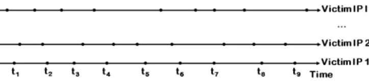
(a) Illustration of victim-level stochastic cyber attack processes with respect to individual victim IP addresses, where dots represent attack events and (for example) attacks against victim IP 1 arrive at timet1, . . . , t9.
(b) Elaboration of a victim-level attack process with respect to victim IP 1. Fig. 1. Illustration of victim-level stochastic cyber attack processes
Figure 1(a) illustrates the attacks against individual victim IP addresses, where dots on the same time axis formulate a victim-level attack process. Figure 1(b) further shows that a victim is attacked by N attackers (or attacking computers) at some ports and the attacks arrive at time t1, . . . , t9.
B. The Framework
The framework is presented as a 5-step procedure. Step 1 (data pre-processing) is presented for completeness because the data may be collected by software or hardware. Step 2 (basic statistical analysis) serves the purpose of providing hints for Step 3 (advanced statistical analysis for identifying statisti-cal properties of attack processes), which in turn serves as the base for Step 4 (“gray-box” prediction) and Step 5 (exploring the cause of the newly identified statistical properties).
Step 1: Data pre-processing: It is now a common practice to treat honeypot-captured data as attacks because there are no legitimate services and the honeypot computers passively wait for incoming events. Honeypot-captured cyber attack data is often organized according to the honeypot IP addresses. Pre-processing mainly deals with two issues. First, we may need to differentiate the attack traffic corresponding to the production portsthat are associated to some honeypot programs/services, and the attack traffic corresponding to the non-production ports that are not associated to any services.
Second, in order to analyze statistical properties exhibited by honeypot-captured cyber attack data, we advocate using
flows, rather than IP packets, to represent attacks because of the following. (i) For low-interaction honeypots data, attack payload is often missing and information about attacks is often captured from the perspective of communication behaviors. This suggests that flow is appropriate for analyzing honeypot-captured cyber attack data. (ii) Flow-based intrusion detection is complementary to the traditional packet-based intrusion detection. For example, flow-based abstraction can be used to detect attacks such as DoS (denial-of-service), scan, worm [10], [11]. (iii) Flow-based abstraction can deal with encrypted attack payload [12], which cannot be dealt with by packet-level analysis.
The concept of flow accommodates both TCP and UDP. There are COTS devices that can readily extract flows. How-ever, when honeypot data is collected by software in the format ofpcapdata, we need to parse it and re-assemble into flows. Since flow assembly is a standard technique, in what follows we only briefly review the assembly of TCP flows. A TCP flow is uniquely identified from honeypot-collected raw pcap data via the attacker’s IP address, the port used by the attacker, the victim IP address in the honeypot, and the port that is under attack. An unfinished TCP handshake can also be treated as a flow (attack) because an unsuccessful handshake can be caused by events such as: the port in question is busy (i.e., the connection is dropped). For flows that do not end with the FIN flag (which would indicate safe termination of TCP connection) or the RST flag (which would indicate unnatural termination of TCP connection), we need to choose two parameters in the pre-processing. One parameter is the flow timeout time, meaning that a flow is considered expired when no packet of the flow is received during a time window. For example, 60 seconds would be reasonable for low-interaction honeypots that provide limited interactions [13], but a longer time may be needed for high-interaction honeypots. The other parameter is theflow lifetime, meaning that a flow is considered expired when a flow lives longer than a pre-determined lifetime, which can be set as 300 seconds for low-interaction honeypots [13] but a longer time may be needed for high-interaction honeypots.
Step 2: Basic statistical analysis: The basic statistics of cyber attack data can offer hints for advanced statistical analysis. For stochastic cyber attack processes, the primary statistic is the attack rate, which describes the number of attacks that arrive at unit time (e.g., minute or hour or day). Note that attack rate can be instantiated at various resolutions of attack processes, such as: network-level attack rate, victim-level attack rate and port-victim-level attack rate. The secondary statistic is the attack inter-arrival time, which describes the time intervals between two consecutive attack events. By investigating the min, mean, median, variance and max
of these statistics, we can identify outliers and obtain hints about the properties of the attack processes. For example, if the attack events are bursty, an attack process may not be Poisson, which can serve as a hint for further advanced statistical analysis.
Step 3: Advanced statistical analysis: Identifying sta-tistical properties of attack processes: This step is to identify statistical properties of attack processes at resolutions
of interest. A particular question that should be asked is: Are the attack processes Poisson? Recall that the Poisson process counts the number of events that occur during time intervals, where “events” in the context of this paper are the attacks observed by honeypots. If not Poisson, what properties do they exhibit? It would be ideal that the attack processes are Poisson because we can easily characterize Poisson processes with very few parameters, and because there are many mature methods and techniques for analyzing them. For example, we can use the property — the superposition of Poisson processes is still a Poisson process [14] — to simplify problems when we consider attack processes at multiple resolutions/levels. In many cases, attack processes may not be Poisson. For characterizing such processes, we need to use advanced sta-tistical methods, such as Markov process, L´evy process, and time-series methods [9], [15]. This step is crucial because identifying advanced statistical properties can pave the way for answering the next questions. This step can be quite involved in terms of statistical skills when the attack processes are not Poisson.
Step 4: Exploiting the statistical properties: This step addresses the following question: How can we exploit the statistical properties of stochastic cyber attack processes to do useful things? One exploitation is to conduct “gray-box” prediction of the incoming attacks, at least in terms of attack rate at the appropriate resolution (which in turn depends on the data is collected by low-interaction or high-interaction honeypot). By “gray-box” prediction we mean that if an attack process exhibits a certain property that is identified in Step 3 (e.g., Long-Range Dependence [1], [2] or Short-Range Dependence [15], [3]), the prediction model should accommodate the property as well. Algorithm 1 describes a general “gray-box” prediction algorithm, where{X1, . . . , Xt}
is the sequence of attack rates observed at time1, . . . , t, andh is the number of steps (e.g., hours) we want to predict ahead of time. In addition to “gray-box” prediction, Algorithm 1 is novel also because it selects the best model (from a family of models) at each prediction step, which is important because there may be no single model that can fit the observed data well at all steps.
Algorithm 1 Prediction Algorithm
INPUT: observed attack rates{X1, . . . , Xt},h(steps ahead)
OUTPUT: prediction results Yt+h, Yt+h+1, . . .
1: repeat
2: Fit{X1, . . . , Xt} to obtain the best modelMt from a
family of models that accommodate the newly identified statistical properties (i.e., “gray-box” prediction) with respect to an appropriate model selection criterion (e.g., Akaike information criterion (AIC) [7])
3: UseMtto predictYt+h, the number of attacks that will
arrive during the(t+h)th step
4: Xt+1←newly observed attack rate at time t+ 1
5: t←t+ 1 {observing more data ast evolves}
6: untilno need to predict further
We note that although the prediction is geared toward
honeypot-oriented traffic, it can be useful for defending pro-duction networks as well. This is because when honeypot-captured attacks are increasing (or decreasing), the attack rate with respect to production networks might also be increasing (or decreasing) as long as the honeypots are approximately uniformly deployed in the IP address space in question. This can be achieved by blending honeypot IP addresses into production IP addresses. Since being able to predict incoming attacks (especially hours ahead of time) is always appealing, this would give incentives to deploy honeypots as such. As a result, it is possible to characterize the relation between the attack traffic into the honeypot IP addresses and the attack traffic into the production IP addresses.
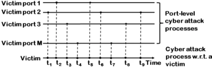
(a) Decomposition of a victim-level attack process into multiple port-level attack processes, where the attack process corresponding to Port 1 describes the attacks that arrive at timet2 andt5, the attack process corresponding to
Port 2 describes the attacks that arrive at timet1,t6andt9, etc.
(b) Attacker-level attack process can be derived from victim-level attack process by ignoring the subsequent attacks launched by the same attacker. In this example, the attacker-level attack process corresponding to the victim describes the attacks that arrive at timet1, t2, t3, t4.
Fig. 2. Two approaches to exploring causes of statistical properties
Step 5: Exploring cause of the statistical properties:
This step aims to address the following question: What caused the statistical properties exhibited by stochastic cyber attack processes? This question is interesting because it reflects a kind of “natural” phenomenon in cyberspace. It would be ideal that one can mathematically prove the cause of a property. This type of “theoretical proof” approach is often difficult, as witnessed by the outcome of the past two decades of effort at studying the long-range dependence exhibited by benign Internet traffic (see Section VI). Therefore, we advocate the “experimental” approach, which includes the following two specific methods. The first method is to study the decomposed lower-level (i.e., higher-resolution) stochastic cyber attack processes. For example, in order to investigate whether or not a certain property is caused by another certain property of the low-level (i.e., high-resolution) processes, we can decompose a victim-level attack process into port-level attack processes that correspond to the individual ports of the victim. This is illustrated in Figure 2(a), where the victim-level attack process is decomposed into M port-level attack processes.
The second method is to investigate whether or not a certain property is caused by the intense (consecutive) attacks that are launched by individual attackers. For this purpose, we can consider the attacks against each victim that are launched by distinct attackers. As illustrated in Figure 2(b), even though an attacker launched multiple consecutive attacks against a victim, we only need to consider the first attack. If the attacker-level attack processes do not exhibit the property that is exhibited by the victim-level attack processes, we can conclude that the property is probably caused by the intensity of the attacks that are launched by individual attackers.
IV. CASESTUDY
To demonstrate use of the framework, we conduct a case study by applying it to analyze a dataset that was collected by a low-interactionhoneypot. As mentioned above, the framework can be equally applied to analyze high-interaction honeypot data.
A. Data Pre-Processing
The dataset for our case study was collected by a honeypot, which ran four popular low-interaction honeypot software programs: Dionaea [16], Mwcollector [17], Amun [18], and Nepenthes [19]. The vulnerable services offered by all four honeypot programs are SMB, NetBIOS, HTTP, MySQL and SSH, each of which is associated to a unique TCP port. These are the production ports. Each honeypot IP address was assigned to one of these programs and was completely isolated from the other honeypot IP addresses. A single honeypot computer was assigned with multiple IP addresses to run multiple honeypot software programs. A dedicated computer was used to collect the raw network traffic as pcap files, which were timestamped at the resolution of microsecond. Table I summarizes the dataset, which corresponds to 166 victim/honeypot IP addresses for five periods of time. These periods are not strictly consecutive because of network/system maintenance etc.
Period Dates Duration
(days) # victim IPs I 11/04/2010 - 12/21/2010 47 166 II 02/09/2011 - 02/27/2011 18 166 III 03/12/2011 - 05/06/2011 54 166 IV 05/09/2011 - 05/30/2011 21 166 V 06/22/2011 - 09/12/2011 80 166 TABLE I DATA DESCRIPTION
In our pre-processing, we resolve the two issues described in the framework as follows. First, we disregard the attacks against the non-production ports because such TCP connec-tions are often dropped. Note that the specific attacks against the production ports are dependent upon the vulnerabilities emulated by the honeypot programs (e.g., Microsoft Windows Server Service Buffer Overflow MS06040 and Workstation Service Vulnerability MS06070 for the SMB service). Since low-interaction honeypots do not capture sufficient informa-tion for precisely recognizing the specific attacks, we do not look into specific attack types. Second, for flows that do not
end with the FIN flag (indicating safe termination of TCP connection) or the RST flag (indicating unnatural termination of TCP connection), we use the following two parameter values: 60 seconds for theflow timeout timeand 300 seconds for theflow lifetime.
B. Basic Statistical Analysis
We consider theper-hourattack rate at three resolutions: the honeypot network, individual victim IP address, and individual production port of each victim. The choice of per-hour is natural, while noting thatper-dayattack rate is not appropriate because each period is no more than 80 days. Since the numbers of victim-level and port-level attack processes are much larger than the number of network-level attack processes, different methods are used to represent their basic statistics.
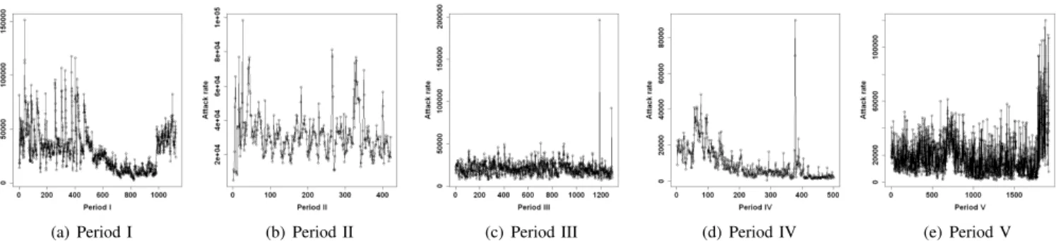
Basic statistics of network-level attack processes: For network-level attack processes, it is feasible and appropriate to plot the time series of the attack rate (per hour), namely the total number of attacks against the honeypot network of 166 victims. Figure 3 plots the time series of attacks. We make the following observations. First, the five periods exhibit different attack patterns. For example, Periods I, II and V are relatively stationary. Second, there are some extremely intense attacks during some hours in Periods III and IV. The specific hour corresponding to the extreme value in Period III is Apr 01, 2011, 12 Noon (US Eastern Time); the attacks are against the SSH services. It is evident that the attacks are brute-forcing password. The peak of attacks during Period IV occurs at May 16, 2011, 3 AM (US Eastern Time). The intense attacks are against the HTTP service. We find no information from the Internet whether or not there are worm/botnet outbreaks that correspond to the peaks. Third, although the five plots exhibit some change-points, a formal statistical analysis (using the method reviewed in Section II for removing spurious LRD) shows that change-points exist only in Period III, which correspond to the largest attack rate. This means that visual observations can be misleading and rigorous statistical analysis is perhaps necessary.
Table II describes the basic statistics of the network-level attack rate. On average, the victim network is least intensively attacked during Period IV because the average per-hour attack rate is about 9861, which is smaller than the average attack rate during the other periods. The variances of attack rates are much larger than the corresponding mean attack rates, whichhintsthat these processes are not Poisson. As we show via formal statistical analysis in Section IV-C, these processes actually exhibit LRD instead.
Period MIN Mean Median Variance Max
I 2572 30963.2 28263 401243263.2 151189 II 5155 31576.8 29594 167872819.0 98527 III 6732 20382.3 19579 72436071.5 196210 IV 637 9861.1 6528 93209085.3 89718 V 1417 18960.2 15248.5 205276388.4 120221 TABLE II
BASIC STATISTICS OF NETWORK-LEVEL ATTACK PROCESSES.
Basic statistics of victim-level attack processes: For victim-level attack processes, we consider the attack rate or
(a) Period I (b) Period II (c) Period III (d) Period IV (e) Period V Fig. 3. Time series plots of the network-level attack processes. Thex-axis indicates the relative time with respect to the start time for each period (unit: hour). They-axis indicates attack rate, namely the number of attacks (per hour) arriving at the honeypot.
the number of attacks (per hour) arriving at a victim. Since there are 166 victims in each period, we cannot afford to plot time series of victim-level attack processes.
Period Mean(·) Median(·) Variance(·) MAX(·)
LB UB LB UB LB UB LB UB I 32.1 1810.4 8 1327 1589.9 3219758.8 247 14403 II 49.8 1412.0 43 1112 1466.5 1553585.6 335 10995 III 11.5 1513.5 3 1490 254.0 676860.7 125 5287 IV 3.5 1663.4 1 1184 29.7 2808045.2 41 7793 V 34.0 2228.8 8.5 1526.5 1225.6 4639659.1 274 12267 TABLE III
BASIC STATISTICS OF VICTIM-LEVEL ATTACK PROCESSES:ATTACK RATE (PER HOUR). FOR A SPECIFIC PERIOD AND A SPECIFIC STATISTIC X∈ {Mean,Median,Variance,MAX}, LB (UB)STANDS FOR THE
LOWER-BOUND OR MINIMUM(UPPER-BOUND OR MAXIMUM)OF STATISTICXAMONG ALL THE VICTIMS AND ALL THE HOURS. IN OTHER
WORDS,THELBANDUBVALUES REPRESENT THE MINIMUM AND MAXIMUM PER-HOUR ATTACK RATE OBSERVED DURING AN ENTIRE
PERIOD AND AMONG ALL THE VICTIMS.
Table III summaries the observed lower-bound (minimum) and upper-bound (maximum) values of per-hour attack rate for each statistic among the 166 victims. By taking Period I as an example, we observe the following. The average per-hour attack rate (among all the victims and among all the hours) is 32–1810 attacks per hour; the median per-hour attack rate is 8–1327 attacks per per-hour; the maximum number of attacks against a single victim can be up to 14403. Boxplots of the four statistics, which are not included for the sake of saving space, show that the five periods exhibit somewhat similar (homogeneous) statistical properties. For example, each statistic has many outliers in each period. By looking into all individual victim-level attack processes, we find that among all the 830 victim-level attack processes (166 victims/period × 5 periods = 830 victims), the variance of attack rate is at least 3.5 times greater than the mean attack rate corresponding to the same victim. This fact — the variance is much larger than the mean attack rate — hints that Poisson models may not be appropriate for describing victim-level attack processes. This suggests us to conduct formal statistical tests, which will be presented in Section IV-C.
Basic statistics of port-level attack processes: For port-level attack processes, Table IV summarizes the lower-bound (minimum value) and upper-lower-bound (maximum value) for each statistic. By taking Period I as an example, we observe the following. There can be no attacks against some production ports during some hours, which explains why the
Meanper-hour attack rate can be 0. On the other hand, a port
(specifically, port 445 at Nov 6, 2010, 9 AM US Eastern time) can be attacked by 14363 attacks within one hour. Like what is observed from the victim-level attack processes, we observe that the variance of attack rate is much larger than the mean attack rate. This means that the port-level attack processes are not Poisson. Indeed, as we will see in Section IV-E, many port-level attack processes are actually heavy-tailed.
Period Mean(·) Median(·) Variance(·) MAX(·)
LB UB LB UB LB UB LB UB I 0 1740.7 0 1196 0 3249318.9 1 14363 II 0 1251.5 0 948 0 1545078.5 1 10992 III 0 1482.1 0 1458 0 661847.3 1 5275 IV 0 1613.4 0 1142 0 2588396.6 1 6961 V 0 2169.8 0 1448.5 0 4629744.3 1 12267 TABLE IV
BASIC STATISTICS OF PORT-LEVEL ATTACK PROCESSES:ATTACK-RATE (PER HOUR). AS INTABLEIII, LBANDUBVALUES REPRESENT THE MINIMUM AND MAXIMUM PER-HOUR ATTACK RATE OBSERVED DURING
AN ENTIRE PERIOD AND AMONG ALL PRODUCTION PORTS OF THE VICTIMS.
C. Identifying Statistical Properties of Attack Processes We now characterize the statistical properties exhibited by network-level and victim-level attack processes. In particular, we want to know they exhibit similar (if not exactly the same) or different properties. In the above, we are already hinted that the attack processes are not Poisson. In what follows we aim to pin down their properties.
Network-level attack processes exhibit LRD: The hint that network-level attack processes are not Poisson suggests us to identify their properties. It turns out that the network-level attack processes exhibit LRD as demonstrated by their Hurst parameters. Table V describes the six kinds of Hurst pa-rameters corresponding to the network-level attack processes. Although the Hurst parameters suggest that they all exhibit LRD, a further analysis shows the LRD exhibited in Period III is spurious because it was caused by the non-stationarity of the process. Therefore, 4 out of the 5 network-level attack processes exhibit (legitimate) LRD.
Victim-level attack processes exhibit LRD: For the 830 (166 victims/period×5 periods =830) victim-level attack processes, we first rigorously show that they are not Poisson. Assume that the attack inter-arrival times are independent and identically distributed exponential random variables with distribution
Period RS AGV Peng Per Box Wave LRD? I 0.80 0.95 0.88 1.03 1.00 0.75 Yes II 0.74 0.59 0.86 0.75 0.97 0.84 Yes III 0.74 0.52 0.65 0.63 0.63 0.65 No IV 1.05 0.97 0.95 1.07 0.97 1.22 Yes V 0.74 0.78 0.74 1.03 0.80 0.80 Yes TABLE V
THE ESTIMATEDHURST PARAMETERS FOR NETWORK-LEVEL ATTACK PROCESSES. THE SIX ESTIMATION METHODS ARE REVIEWED INAPPENDIX
A-A. NOTE THAT AHURST PARAMETER VALUE BEING NEGATIVE OR BEING GREATER THAN1MEANS THAT EITHER THE ESTIMATION METHOD
IS NOT SUITABLE OR THE ATTACK PROCESS IS NON-STATIONARY.
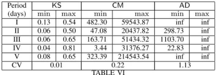
To test the exponential distribution, we first estimate the unknown parameter λ by the maximum likelihood method. Then, we compute the Kolmogorov-Smirnov (KS), Cram´er-von Mises (CM), and Anderson-Darling (AD) test statistics [20], [21] (cf. Appendix A-C for a review) and compare them against the respective critical values.
Period KS CM AD
(days) min max min max min max
I 0.13 0.54 482.30 59543.87 inf inf II 0.06 0.50 47.08 20437.82 298.73 inf III 0.06 0.65 163.71 51434.32 1103.70 inf IV 0.04 0.81 3.44 31376.27 22.83 inf V 0.08 0.65 323.39 214543.54 inf inf CV 0.01 0.22 1.13 TABLE VI
MINIMUM VALUES OF THE THREE TEST STATISTICS FOR ATTACK INTER-ARRIVAL TIME(UNIT:SECOND)CORRESPONDING TO THE VICTIM-LEVEL ATTACK PROCESSES,WHEREminANDmaxREPRESENT
THE MINIMAL AND MAXIMAL MINIMUM VALUES AMONG ALL VICTIM-LEVEL ATTACK PROCESSES IN A PERIOD,ANDInfMEANS THE
VALUE IS EXTREMELY LARGE.
Table VI reports the minimum test statistics, where the critical values for the test statistics are based on significance level .05 and obtained from [22], [23]. Since the values are far from the critical values, there is no evidence to support the exponential distribution hypothesis. Because the minimum test statistics violate the exponential distribution assumption already, greater test statistics must violate the exponential distribution assumption as well.
(a) QQ-plot of inter-arrival time of victim-level attack process that ex-hibits the minimum KS, CM and AD value simultaneously
(b) Boxplot of Hurst parameters of attack rate of the victim-level attack processes corresponding to the 5 pe-riods
Fig. 4. Victim-level attack processes are not Poisson but exhibit LRD We also use QQ-plot to evaluate the goodness-of-fit of expo-nential distributions for the attack inter-arrival time of victim-level attack processes that simultaneously exhibit the minimum test statistics in Table VI. This is the victim from Period IV
withHKS= 0.04,HCM= 3.44andHAD = 22.83. If the attack
inter-arrival time corresponding to this particular victim does not exhibit the exponential distribution, we conclude that no attack inter-arrival time in this dataset exhibits the exponential distribution. The QQ plot is displayed in Figure 4(a). We observe a large deviation in the tails. Hence, exponential distribution cannot be used as the distribution of attack inter-arrival times, meaning that all the victim-level attack processes are not Poisson.
Given that the victim-level attack processes are not Poisson, we suspect they might exhibit LRD as well. Figure 4(b) shows the boxplots of Hurst parameters of attack rate. We observe that Periods I and II have relatively large Hurst parameters, suggesting stronger LRD. Table VII summarizes the minimums and maximums of the estimated Hurst param-eters of attack rates. Consider Period I as an example, we observe that the attack processes corresponding to 163 (out of the 166) victims have average Hurst parameters falling into
[.6,1]and thus suggest LRD, where the average is taken over the six kinds of Hurst parameters. However, only 159 (out of the 163) victim-level attack processes exhibit legitimate LRD because the other 4 (out of the 163) victim-level attack processes are actually spurious LRD (i.e., caused by the non-stationarity of the processes). We also observe that in Period III, there are only 87 victim-level attack processes that exhibit LRD. Overall, 70% victim-level attack processes, or
159 + 116 + 87 + 125 + 89 = 576out of166×5 = 830attack processes, exhibit LRD.
Port-level attack processes exhibit LRD: Table VIII summarizes the Hurst parameters of port-level attack pro-cesses. We observe that there are respectively 316, 397, 399, 328, 406 port-level attack processes that exhibit LRD. Since there are 5 production ports per victim and 166 victims, there are 830 port-level attack processes per period. Since there are 5 periods of time, there are 4150 port-level attack processes in total (830 ports/period× 5 periods=4150 ports). This means that (316 + 397 + 399 + 328406)/4150 = 44.5% port-level attack processes exhibit LRD.
Summary: In summary, we observe that 80% (4 out of 5) network-level attack processes exhibit LRD, 70% victim-level attack processes exhibit LRD, and 44.5% port-victim-level attack processes exhibit LRD. This means that defenders should expect that the burst of attacks will sustain, and that cyber attack processes should be modeled using LRD-aware stochastic processes.
D. Exploiting LRD to Predict Attack Rates
Assuming that the attacks arriving at honeypots are repre-sentative of, or related to, the attacks arriving at production networks (perhaps in some non-trivial fashion that can be identified given sufficient data), being able to predict the number of incoming attacks hours ahead of time can give the defenders sufficient early-warning time to prepare for the arrival of attacks. Intuitively, the model that is good at prediction in this context should accommodate the LRD property. This is confirmed by our study described below.
Period RS AGV Peng Per Box Wave # victims w/ # victims w/ min max min max min max min max min max min max H¯ ∈[.6,1] LRD I 0.53 1.01 0.46 0.98 0.66 1.14 0.73 1.39 0.55 1.15 0.40 0.96 163 159 II 0.49 0.94 0.40 0.98 0.56 1.37 0.53 1.69 0.33 1.32 -0.55 1.33 130 116 III 0.65 0.95 0.30 0.96 0.53 1.06 0.44 1.22 0.43 0.98 0.33 1.02 93 87 IV 0.40 1.13 0.12 1.00 0.49 1.45 0.33 1.74 0.42 1.32 -0.34 1.47 126 125 V 0.52 1.01 0.14 0.99 0.45 1.22 0.47 1.43 0.57 1.30 -0.16 1.18 158 89 TABLE VII
THE ESTIMATEDHURST PARAMETERS FOR ATTACK RATE(PER HOUR)OF THE VICTIM-LEVEL ATTACK PROCESSES. THE SIX ESTIMATION METHODS ARE REVIEWED INAPPENDIXA-A. NOTE THAT AHURST VALUE BEING NEGATIVE OR BEING GREATER THAN1MEANS THAT EITHER THE ESTIMATION METHOD IS NOT SUITABLE OR THE PROCESS IS NON-STATIONARY. THE COLUMN“#OF VICTIMS W/H¯ ∈[.6,1]”REPRESENTS THE TOTAL NUMBER OF
VICTIM-LEVEL ATTACK PROCESSES WHOSE AVERAGEHURST PARAMETERS∈[.6,1](WHERE AVERAGE IS AMONG THE SIX KINDS OFHURST PARAMETERS),WHICH SUGGESTS THE PRESENCE OFLRD. THE COLUMN“#OF VICTIMS W/ LRD”INDICATES THE TOTAL NUMBER OF VICTIM-LEVEL ATTACK PROCESSES THAT EXHIBITLRDRATHER THAN SPURIOUSLRD. (THE SAME NOTATIONS WILL BE USED IN THE DESCRIPTION OFTABLESVIII
ANDXIII.)
Period RS AGV Peng Per Box Wave total # of # ports w/ # ports w/
min max min max min max min max min max min max ports H¯ ∈[.6,1] LRD I 0.41 1.01 -0.18 0.98 -0.15 1.23 0.38 1.55 0.39 1.48 -0.18 1.00 830 + 0 349 316 II 0.23 1.50 0.04 0.97 0.18 1.51 0.32 1.68 0.26 1.45 -0.60 1.38 829 + 1 419 397 III 0.14 1.01 -0.02 0.96 0.27 1.08 0.38 1.28 0.34 1.07 0.08 1.00 830 + 0 422 399 IV 0.25 1.17 0.05 1.00 0.24 1.57 0.18 1.70 0.29 1.50 -1.10 1.72 828 + 2 339 328 V 0.43 1.14 0.12 0.99 0.42 1.40 0.45 1.52 0.40 1.41 -1.07 1.43 830 + 0 528 406 TABLE VIII
THE ESTIMATEDHURST PARAMETERS FOR PORT-LEVEL ATTACK RATE(PER HOUR)OF THE PORT-LEVEL ATTACK PROCESSES.
Prediction results for network-level attack processes:
In order to evaluate the accuracy of the prediction results, we use Algorithm 2, which is an instantiation of Algorithm 1 while considering prediction errors for evaluation purpose. Let {X1, . . . , Xn} be the time series of observed attack
rates. Algorithm 2 uses portion of the observed attack rates
{X1, . . . , Xn} for fitting a prediction model and compares
the predicted attack rates to the observed attack rates for computing the prediction accuracy, where h be an input parameter indicating the number of steps (i.e., hours) we will predict ahead of time, and pbe another input parameter indicating location of the prediction starting point. In order to build reliable models, we set p= 50%meaning that 50% of the observed data is used as the training data for building models.
Algorithm 2 Prediction Evaluation Algorithm
INPUT: observed attack rates{X1, . . . , Xn},h(hours ahead),
p∈(0,1)indicates prediction start point OUTPUT: prediction accuracy
1: t← bn∗pc 2: while t≤n−hdo
3: Fit {X1, . . . , Xt} to obtain an optimal model Mt as
follows: fit the data to 25 models FARIMA(p, d, q)with varying parameterspandq(which uniquely determine parameter d) and select the best fitting model based on the AIC criterion [7].{The case of ARMA(p, q) is similar.}
4: UseMtto predictYt+h, the number of attacks that will
arrive during the (t+h)th step
5: Compute prediction erroret+h=Xt+h−Yt+h
6: t←t+ 1
7: end while
8: ComputePMAD,PMAD0,OA,UAas defined in Section II-C
9: return PMAD,PMAD0,OA,UA
Now we report the prediction results, while comparing the LRD-aware FARIMA model and the LRD-less ARMA model. Table IX describes the prediction error of the network-level attack processes. We observe the following. First, for Periods I and II, both 1-hour ahead and 5-hour ahead FARIMA prediction errors are no greater than 22%. However, the 10-hour ahead FARIMA prediction is pretty bad. This means that LRD-aware FARIMA can effectively predict the attack rate even five hours ahead of time. This would give the defender enough early-warning time.
Second, Period III network-level attack process exhibits spu-rious LRD. However, both the LRD-aware FARIMA and the LRD-less ARMA models can predict incoming attacks up to 5 hours ahead of time. Indeed, the prediction error of FARIMA
PMAD PMAD0
Period FARIMA ARMA FARIMA ARMA 1-hour ahead prediction (h= 1,p= 0.5)
I 0.179 0.446 0.173 0.157
II 0.217 0.363 0.149 0.149 III 0.298 0.273 0.305 0.312 IV 0.548 0.526 0.126 0.106
V 0.517 0.529 0.424 0.411
5-hour ahead prediction (h= 5,p= 0.5)
I 0.206 0.556 0.292 0.314
II 0.212 0.351 0.420 0.411 III 0.297 0.272 0.246 0.250 IV 0.847 0.838 0.226 0.207
V 0.526 0.555 0.414 0.417
10-hour ahead prediction (h= 10,p= 0.5)
I 0.869 0.801 0.314 0.281 II 1.024 1.034 0.277 0.284 III 1.00 1.002 0.202 0.201 IV 0.648 0.627 0.282 0.490 V 0.982 0.952 0.402 0.412 TABLE IX
PREDICTION ERROR OF NETWORK-LEVEL ATTACK PROCESSES USING THE LRD-AWAREFARIMAAND THELRD-LESSARMA,WHERE PREDICTION ERRORS ARE DEFINED INSECTIONII.p= 0.5MEANS THAT WE START
PREDICTING IN THE MIDPOINT OF EACH NETWORK-LEVEL ATTACK PROCESS.
is slightly greater than the prediction error of ARMA. This reiterates that if an attack process does not exhibit LRD, it is better not to use LRD-aware prediction models; if an attack process exhibits LRD, LRD-aware prediction models should be used. This highlights the advantage of “gray-box” prediction over “black-box” prediction, which demonstrates the principal utility of the statistical framework.
Third, although Period IV exhibits LRD, even its 1-hour ahead FARIMA prediction is not good enough, with prediction error greater than 50%. While it is unclear what caused this effect, we note that the underestimation error PMAD0 for 5-hour ahead prediction is still reasonable for Period IV (22.6% for FARIMA and 20.7% for ARMA). This means that if one is willing to over-provision defense resources to some extent, then the prediction for Period IV is still useful.
Fourth, Period V resists both prediction models in terms of both overall prediction errorPMADand underestimation error PMAD0. The fundamental cause of the effect is unknown at the moment, and is left for future studies. Nevertheless, we suspect that Extreme Value Theory could be exploited to address this problem.
Prediction results for victim-level attack processes:
Since there are 166 victims per period, there are 830 victim-level attack processes for which we will do prediction. Recall that 70% victim-level attack processes exhibit LRD. We use Table X to succinctly present the prediction results, which are with respect to 10-hour ahead predictions during the last 100 hours of each time period. We make the following observations. First, the LRD-aware FARIMA model performs better than the LRD-less ARMA model. For example, among the 152 (out of the 159) victim-level attack processes in Period I that exhibit LRD and are amenable to prediction (i.e., the Maximum Likelihood Estimator actually converges; the Estimator does not converge for 159-152=7 LRD processes though), FARIMA can predict for 29 victim-level attack pro-cesses about their 10-hour ahead attack rates with at least 70%
overall accuracy (OA), while ARMA can only predict for 13 victim-level attack processes at the same level of accuracy. If the defender is willing to over-provision some resources and mainly cares about the underestimation error (which could cause overlooking of attacks), FARIMA can predict for 40 victim-level attack processes while ARMA can predict for 35. Second, the victim-level attack processes in Period I exhibit LRD and render more to prediction when compared with the victim-level attacks processes in the other periods, which also exhibit LRD. For non-LRD processes, neither FARIMA nor ARMA can provide good predictions. This may be caused by the the non-stationary of the non-LRD processes. We plan to investigate into these issues in the future.
Summary: It is feasible to predict network-level attacks even 5 hours ahead of time. For attack processes that exhibit LRD, LRD-aware modelscanpredict their attack rates better than LRD-less models do. However, there are LRD processes that can resist the prediction of even LRD-aware models. This hints that new prediction models are needed.
E. Exploring (Non)Causes of LRD
Despite intensive studies in other settings, the fundamental cause of LRD is still mysterious. One known possible cause of LRD is the superposition of heavy-tailed processes [24], [25], [26]. Another candidate cause of LRD is that some attackers launch intense (consecutive) attacks (e.g., brute-forcing SSH passwords). Now we examine the two candidate causes as described in the framework.
LRD exhibited by network-level attack processes is not caused by heavy-tailed victim-level attack processes:
We want to know whether or not the LRD exhibited by the 4 network-level attack processes during Periods I, II, IV and V are caused by the superposition of heavy-tailed victim-level attack processes. That is, we want to know how many victim-level attack processes during each of the four periods are heavy-tailed. We find that among the vector of
(166,166,166,166)victim-level attack processes during Peri-ods I, II, IV and V, the vector of victim-level attack processes that exhibit heavy-tails is correspondingly(101,0,24,31), by using the POT method that is reviewed in Appendix A-B. This means that Period I is the only period during which majority of victim-level attack processes exhibit heavy-tails. A few or even none processes in the three other periods exhibited heavy-tails. This suggests that LRD exhibited by the network-level attack processes does not have the same cause as what is believed for benign traffic [27].
LRD exhibited by victim-level attack processes is not caused by heavy-tailed port-level attack processes: Now we investigate whether or not the LRD exhibited by victim-level attack processes is caused by that the underlying port-level attack processes exhibit heavy-tails, a property briefly reviewed in Appendix A-B. Table XI shows that only 8% port-level attack processes, or 56 + 80 + 47 + 3 + 32 = 218out of the (159 + 116 + 87 + 125 + 89 = 576) victims × 5 ports/victim = 2880 port-level attack processes, exhibit heavy-tails. Moreover, only 29 (out of the 576) victim-level attack processes have 2 or 3 port-level attack processes that exhibit
total # of victims # of victims # of victims # of victims # of victims # of victims # of victims Period ((x1, x2)/(y)) w/ average w/ average w/ average w/ average w/ average w/ average
OA≥80% OA≥70% OA≥60% UA≥80% UA≥70% UA≥60%
FARIMA ARMA FARIMA ARMA FARIMA ARMA FARIMA ARMA FARIMA ARMA FARIMA ARMA
I LRD: (152,152)/(159) 2 1 29 13 81 66 13 4 40 35 89 68 non-LRD: (7,7)/(7) 0 0 4 4 6 6 1 4 7 6 7 7 II LRD: (109,109)/(116) 0 0 3 2 9 8 2 1 12 6 26 15 non-LRD: (50,49)/(50) 0 0 0 0 0 2 4 1 6 2 13 5 III LRD: (82,82)/(87) 0 0 4 4 8 9 9 5 23 19 50 43 non-LRD: (79,79)/(79) 0 0 0 0 0 0 0 0 10 7 31 24 IV LRD: (118,118)/(125) 0 0 2 2 5 6 2 3 4 6 11 14 non-LRD: (41,39)/(41) 0 0 0 0 0 0 1 0 2 0 4 1 V LRD: (73,73)/(89) 0 0 0 0 2 1 0 1 2 3 16 4 non-LRD: (77,61)/(77) 0 0 0 0 1 1 0 0 1 0 24 15 TABLE X
NUMBER OF VICTIM-LEVEL ATTACK PROCESSES THAT CAN BE PREDICTED BY THELRD-AWAREFARIMAMODEL MORE ACCURATELY THAN THE LRD-LESSARMAMODEL. FOR THE COLUMN“TOTAL#OF VICTIMS((x1, x2)/(y)),”yIS THE TOTAL NUMBER OF VICTIMS THAT EXHIBITEDLRDOR NON-LRD,x1(ORx2)IS TOTAL NUMBER OF VICTIMS(OUT OF THEyVICTIMS)FOR WHICH THEMAXIMUMLIKELIHOODESTIMATOR(MLE)USED IN
THEFARIMA (ARMA)ALGORITHM CONVERGES(I.E.,y−x1ANDy−x2VICTIMS CANNOT BE PREDICTED BECAUSE THEMLEDOES NOT CONVERGE). THE COLUMN“#OF VICTIMS W/AVERAGEOA(ORUA)≥z%”REPRESENTS THE AVERAGE NUMBER OF VICTIMS(OUT OF THEx1ORx2
VICTIMS THAT CAN BE PREDICTED),FOR WHICH THE AVERAGE PREDICTION ACCURACY IS AT LEASTz%IN TERMS OF OVERALL-ACCURACYOA(OR UNDERESTIMATION-ACCURACYUA),WHERE AVERAGE IS OVER ALL PREDICTIONS.
total # of # of victims w/ # of victims with total # Shape # of ports # of ports
Period victims sub-processes certain # of sub-processes of ports mean w/ shape w/ shape Standard exhibiting exhibiting exhibiting heavy-tail exhibiting value value value deviation
LRD heavy-tail 1 2 3 4 5 heavy-tail ∈(.5,1) ≥1 I 159 56 50 6 0 0 0 62 .11 1 0 .11 II 116 80 78 11 1 0 0 103 .40 50 0 .22 III 87 47 39 6 2 0 0 57 .22 2 0 .18 IV 125 3 3 0 0 0 0 3 .43 1 0 .35 V 89 32 29 1 2 0 0 37 .30 5 1 .25 TABLE XI
FOR VICTIM-LEVEL ATTACK PROCESSES EXHIBITINGLRD,SOME PORT-LEVEL ATTACK PROCESSES EXHIBIT HEAVY-TAILS.
heavy-tails. Further, there is only 1 port-level attack process that exhibits infinite mean because the shape value ≥1, and there are1+50+2+1+5 = 59port-level attack processes that exhibit infinite variance because their shape values ∈(.5,1). The above observations also hint that unlike in the setting of benign traffic [27], LRD exhibited by victim-level attack processes is not caused by the superposition of heavy-tailed port-level attack processes.
LRD exhibited by victim-level attack processes is not caused by individual intense attacks: Now we examine whether or not LRD is caused by the individual attackers that launch intense attacks. For this purpose, we consider attacker-level attack processes, which model the attacks against each victim that are launched bydistinctattackers. In other words, we only consider the first attack launched by each attacker, while disregarding the subsequent attacks launched by the same attacker.
Table XII describes the observed lower-bound and upper-bound of the four statistics regarding the attacker-level pro-cesses, where the bounds are among all victims within a period of time. By taking Period II as an example, we observe the following: on average there are between 48 and 100 attackers against one individual victim within one hour, and there can be up to 621 attackers against one individual victim within one hour. Further, attacks in Periods III and IV exhibit different behaviors from the other three periods. From the boxplots of the basic statistic, which are not presented for the sake of saving space, we observe that the attackers’ behaviors are actually very different in the 5 periods. In particular, the
attacker-level attack processes in Period II have many outliers in terms of the four statistics, meaning that the attack rate during this period varies a lot.
Period Mean(·) Median(·) Variance(·) MAX(·)
LB UB LB UB LB UB LB UB I 30.2 67.8 4 45 1498.1 4094.3 225 432 II 48.6 100.8 42 93 1195.1 6298.3 306 621 III 11.1 33.0 2 29 223.6 270.8 64 100 IV 1.9 23.8 1 23 26.32 92.7 40 65 V 33.4 127.9 8 105 1132.7 7465.2 266 605 TABLE XII
BASIC STATISTICS OF ATTACK RATE OF THE ATTACKER-LEVEL ATTACK PROCESSES(PER HOUR).
In order to see whether or not the attacker-level attack processes still exhibit LRD, we describe their Hurst parameters in Table XIII. Using Period I as an example, we observe that the attacker-level attack processes corresponding to 153 (out of the 166) victims suggest LRD because their average Hurst parameter ∈ [.6,1], where the average is taken over the six Hurst estimation methods. Moreover, none of the 153 attacker-level processes exhibit spurious LRD. Using Period V as another example, we observe that all 166 attacker-level attack processes have average Hurst parameter∈[.6,1], but only 77 attacker-level attack processes exhibit LRD while the other 89 attacker-level attack processes exhibit spurious LRD (caused by non-stationarity of the processes). The above discussion suggests that LRD exhibited by victim-level attack processes is not caused by the intense (consecutive) attacks launched by individual attackers, simply because most (or many)
attacker-Period RS AGV Peng Per Box Wave # victims w/ # victims w/ min max min max min max min max min max min max H¯ ∈[.6,1] LRD I 0.593 0.977 0.851 0.958 0.896 1.111 1.174 1.334 0.942 1.185 0.582 0.843 153 153 II 0.570 0.883 0.616 0.950 0.689 1.070 0.710 1.152 0.663 1.242 -0.360 0.728 92 77 III 0.776 0.994 0.364 0.747 0.630 0.748 0.460 0.679 0.608 0.746 0.389 0.668 163 103 IV 0.657 0.920 0.273 0.955 0.690 0.872 0.559 1.206 0.612 0.952 0.288 1.004 166 165 V 0.495 0.758 0.563 0.727 0.499 0.806 0.898 1.114 0.660 0.977 0.567 0.931 166 77 TABLE XIII
THE ESTIMATEDHURST PARAMETERS OF THE ATTACK RATE OF ATTACKER-LEVEL ATTACK PROCESSES(PER HOUR).
level attack processes also exhibit LRD.
Summary: The LRD exhibited by stochastic cyber attack processes is neither necessarily caused by the superposition of heavy-tailed processes, nor necessarily caused by the intense attacks launched by individual attackers. While we ruled out these two candidate causes, it is an interesting and challenging future work to precisely pin down the cause of LRD in this context.
V. DISCUSSION
In this section we discuss the limitation of the case study and the usefulness of the statistical framework.
A. Limitation of the Case Study
The case study has three limitations that are imposed by the specific dataset. First, the dataset, albeit over47+18+54+21+ 80 = 220days in total (5 periods of time), only corresponds to 166 honeypot IP addresses. We wish to have access to bigger datasets. Still, this paper explores an important direction in cyber security research, especially the feasibility of predicting incoming attacks. Fortunately, the statistical framework can be adopted by researchers to analyze their (bigger) datasets.
Second, the dataset is attack-agnostic in the sense that we know the ports/services the attackers attempt to attack, but not the specific attacks because the data was collected using low-interaction honeypots. Although this issue can be resolved by using high-interaction honeypots [28], there are legitimate concerns about high-interaction honeypots from a legal perspective. Nevertheless, the framework is equally appli-cable to analyze high-interactive honeypot data. For example, there might be researchers who have collected high-interaction honeypot data and are not allowed to share the data with others. These researchers can adopt the framework to analyze their data at a finer resolution (e.g., the attack level that an attack process can accommodate one or multiple families of attacks).
Third, the data is collected using honeypot rather than using production network. For real-life adoption of the prediction capability presented in the paper, attack traffic would be blended into the production traffic. Whether or not the blended traffic also exhibits LRD is an interesting future study topic. The main challenge again is the legal and privacy concerns in collecting such data.
B. Usefulness of the Statistical Framework
The usefulness of the statistical framework (or analysis methodology) can be seen from the following perspectives.
First, the framework hasdescriptivepower because it aims to study the advanced statistical properties exhibited by the cyber attack data that instantiates stochastic cyber attack process. The advanced statistical properties are not known a prior. In order to obtain hints for the kinds of advanced statisti-cal properties that may be relevant, the framework starts at studying basic statistical properties exhibited by the data. The hinted statistical properties are rigorously examined by using advanced statistical techniques, which fall into the framework of Hypothesis Testing (e.g., whether LRD is exhibited or not is tested based on the values of the Hurst parameters that are estimated using the rigorous statistical methods reviewed in Appendix A-A). Indeed, the framework guided us to identify the relevance of LRD in this aspect of cyber security, which is not known until now.
Second, the framework has predictive power because, as confirmed by the case study, it allows to exploit the newly identified advanced statistical properties to predict the attack rate possibly hours ahead of time. This kind of property-inspired “gray-box” prediction, rather than “black-box” pre-diction, allows the defender to proactively provision defense resources. Although the specific dataset used in our case study is collected by a low-interaction honeypot, the concept of stochastic cyber attack process can equally describe the attacks that are observed at high-interaction honeypots. Since high-interaction honeypots can collect more information about attacks, the framework can be equally applied to analyze the data with respect to specific attacks. As a result, we can predict the arrival rate of specific attacks (i.e., attack-centric rather than computer/network-centric). Moreover, the framework in principle could model and predict the emergence of new at-tacks (e.g., zero-day exploits), assuming the data exhibits LRD or other relevant statistical properties that can be exploited for predicting the emergence of new attacks (e.g., the probability that a zero-day attack will arrive at a honeypot, assuming that the data indeed contains new or zero-day attacks). Although we do not have access to high-interaction honeypot data, there would be researchers/practitioners who have access to such data. This explains why we are automating our analysis methodology, and will release the software package so that other researchers/practitioners can use our software package as is, or can enhance it to incorporate more analysis methods to better serve their purposes.
Third, the framework can be adapted to describe attacks against production networks/computers, because identifying statistical properties of the traffic would allow the defender to detect anomalies. For example, suppose the traffic during the past days does not exhibit LRD property (or any other
relevant statistical property) but the traffic today exhibits LRD property, then this hints possible attacks today. Suppose further that a firewall is installed to filter out the known attacks against the production networks/computers. Then the change in statistical properties exhibited by the traffic hints the presence of new (possibly zero-day) attacks against the production networks/computers. These hints serve as clues for further forensics examinations. Note that for further forensics examination of the actually attacks, we need the detailed information about the traffic. Such information is not cap-tured by low-interaction honeypots, but can be capcap-tured by high-interaction honeypots and production defense systems. This explains the limitation of our case study, although the limitation is not inherent to our framework (as it is imposed by the specific dataset collected by low-interaction honeypot). Fourth, consider the scenario that the honeypot IP addresses are randomly scattered into a production network (rather than being allocated to a consecutive chunk of IP addresses). This would be the ideal scenario for deploying honeypots, because it can be hard for the attacker to figure out which IP addresses are the honeypot IP addresses. This is true especially when the honeypot IP addresses are shuffled frequently and randomly and when the honeypot is a high-interaction one. In this case, the attacks arrive at the honeypot IP addresses would be comparable to the attacks that arrive at the production IP addresses. The attacks arrive at the honeypot IP addresses can be equally investigated using the framework presented in the paper. This means that we can predict the arrival rate of the attacks that will come to the honeypot IP addresses possibly hours ahead of time. This also means that we can expect the rate of attacks that will arrive at the production IP addresses hours ahead of time. When the predicted attack rate is high, the defender would need to provision more defense resources to inspect the packets that target the production IP addresses (e.g., for deep packet inspection). The prediction capability gives the defender early-warning that possibly intensive attacks will arrive in the near future. This kind of early-warning capability is desired for real-life defense. Furthermore, the above discussion equally applies to the case that known attacks have been filtered out by firewalls, meaning that the prediction can be with respect to unknown (i.e., new or zero-day) attacks.
VI. RELATEDWORK
We discuss the related prior work from several perspectives. In terms of analyzing honeypot-captured cyber attack data, there have been at least two complementary approaches. One approach is to visualize cyber attack data, such as using neural projection techniques to visualize the ports observed in honeypot data [29]. However, the widely used approach is statistical analysis. Within this approach, existing studies mainly focused on the following aspects: (i) analyzing at-tackers’ probing activities [30]; (ii) grouping attacks (e.g., [31], [13], [32], [33], [34]); (iii) characterizing Internet threats [35], [36] such as fitting the attack inter-arrival time via a mixture of Pareto and Exponential distributions. These studies are often based on flow-level processing of data, so do we in this paper. In contrast to these studies, we systematically
study the identification, exploitation and cause of statistical properties exhibited by honeypot data, such as LRD that is shown to be exhibited by honeypot data for the first time in the present paper. To our knowledge, our framework is the first formal statistical analysis of honeypot-captured cyber attack data. In particular, our study of predicting cyber attacks (in terms of attack rate) would represent a significant step toward the ultimate goal of quantitatively understanding/predicting cyber attacks.
In terms of using honeypots to improve defense, we note that honeypots have been used to help detect various attacks in-cluding DoS (denial-of-service) [37], worms [38], [10], botnets [39], [40], [41], Internet-Messaging threats [42], generating attack signatures [43], [44], and detecting targeted attacks [45]. These studies are important, but are orthogonal to the focus of the present paper.
In terms of the LRD phenomenon, we note that LRD was first observed in benign traffic about two decades ago and there has been a large body of literature on this topic (e.g., [24], [25], [26], [1]). There have been studies on the effect of injecting abnormal events (which are not necessarily attacks) into benign traffics that exhibit LRD. The injection of abnormal events may disrupt the LRD exhibited by the benign traffic (see, e.g., [46]). There also have been studies on the effect of injecting attacks into benign traffics that exhibit LRD (in terms of number of bytes and number of packets). The injection of attack events may not disrupt the LRD (i.e., the “blended” traffics still exhibit LRD) [47]. In the setting of spams, the correlation co-efficient of inter-arrival time of spams that are sent by a group of spammers may decrease slowly, which hints that the inter-arrival time may exhibit LRD [48] — although this was not formally statistically analyzed there. In contrast to all the studies mentioned above, we investigate LRD exhibited byattack ratevia rigorous statistical methods: auto-correlation serves as a hint of possible LRD, Hurst parameters serves as the first rigorous step of examining LRD, and non-stationarity analysis eliminates spurious LRDs. To our knowledge, we are the first to report that LRD is exhibited by honeypot-captured cyber attack data.
Putting data-driven analysis of cyber attacks into a broader context, we note that there have been studies on characterizing blackhole-collected traffic data (e.g., [49], [50]) or one-way traffic in live networks [51]. Still, there are no advanced statistical framework for analyzing such blackhole or one-way traffic data. More specifically, these studies differ from ours in (i) honeypot-captured cyber attack data includes two-way communications, whereas blackhole-collected data mainly cor-responds to one-way communications; (ii) we rigorously ex-plore statistical properties such as LRD, whereas their studies do not pursue such rigorous statistical analysis. Nevertheless, it is possible that our analysis framework can be adapted to analyze blackhole data.
VII. CONCLUSION ANDFUTUREWORK
We introduced the novel concept of stochastic cyber attack process, which offers a new perspective for studying cyber attacks and, in particular, can be instantiated at multiple
resolutions such as network-level, victim-level and port-level. We then proposed a statistical framework that is centered on identifying, exploiting (for “gray-box” prediction) and ex-ploring (for cause analysis) the advanced statistical properties of stochastic cyber attack processes. In order to demonstrate use of the framework, we applied it to analyze some low-interaction honeypot data. The findings of the case study include: (i) majority of the attack processes exhibit LRD; (ii) LRD-aware models can predict the attack rates (especially for network-level attack processes) even 5 hours ahead of time, which would give the defender sufficient early-warning time. The prediction power of the “gray-box” prediction models, when compared with “black-box” prediction models, rewards the effort spent for analyzing the advanced statistical properties of stochastic cyber attack processes.
The present study introduces a range of interesting problems for future research. First, we need to further improve the prediction accuracy, despite that the LRD-aware FARIMA model can predict better than the LRD-less ARMA models. For this purpose, we plan to study some advanced models that can accommodate high volatilities. It is known in the literature that GARCH model may be able to accommodate high volatilities, which has some correlation to LRD. This hints that FARIMA+GARCH models may be able to fit and predict the attack rates better. The other possible way to improve prediction is to incorporate the Extreme Value Theory into the FARIMA process because the FARIMA process may not be able to capture the extremely large attack rate (i.e., the spikes). Second, although our study only ruled out two candidate causes, it is important to rigorously explain the fundamental cause of LRD as exhibited by honeypot-captured cyber attacks. This is a difficult problem in general. Third, the victim-level attack processes and network-level attack processes exhibit similar phenomena (i.e., LRD). This hints a sort of scale-invariancethat, if turns out to hold, would have extremely important implications (for example) in achieving scalable analysis of cyber attacks. Fourth, Wagener et al. [52] recently introduced the concept of adaptive high-interaction honeypots to interact with the attacker strategically, which is reminiscent of [53]. It would be interesting to characterize the statistical properties of such new variants of honeypots. Fifth, one reviewer points out the following interesting research problem: Can we use the information about the prediction errors to directly adjust the prediction results? In order to answer this question, we need to study the statistical properties of the prediction errors.
ACKNOWLEDGEMENT
This study was IRB-approved. We thank the anonymous reviewers for their comments that helped us improve the paper. This work was supported in part by ARO Grant #W911NF-13-1-0141 and AFOSR Grant #FA9550-09-1-0165. Any opinions, findings, and conclusions or recommendations expressed in this material are those of the author(s) and do not necessarily reflect the views of the funding agencies.
REFERENCES
[1] G. Samorodnitsky, “Long range dependence,”Foundations and Trends in Stochastic Systems, vol. 1, no. 3, pp. 163–257, 2006.
[2] W. Willinger, M. Taqqu, W. Leland, and V. Wilson, “Self-similarity in high-speed packet traffic: analysis and modeling of ethernet traffic measurements,”Statistical Sci., vol. 10, pp. 67–85, 1995.
[3] J. Beran,Statistics for Long-Memory Processes. Chapman and Hall, 1994.
[4] T. Mikosch and C. Starica, “Nonstationarities in financial time series, the long-range dependence, and the igarch effects,” The Review of Economics and Statistics, vol. 86, no. 1, pp. 378–390, February 2004. [5] Z. Qu, “A test against spurious long memory,” Boston University -
De-partment of Economics, Boston University - DeDe-partment of Economics - Working Papers Series WP2010-051, 2010.
[6] X. Shao, “A simple test of changes in mean in the possible presence of long-range dependence,”Journal of Time Series Analysis, vol. 32, no. 6, pp. 598–606, November 2011.
[7] J. Cryer and K. Chan,Time Series Analysis With Applications in R. New York: Springer, 2008.
[8] P. Abry and D. Veitch, “Wavelet analysis of long-range-dependent traffic,”IEEE Transactions on Information Theory, vol. 44, no. 1, pp. 2–15, 1998.
[9] D. Daley and D. Vere-Jones,An Introduction to the Theory of Point Processes, Volume 1 (2nd ed.). Springer, 2002.
[10] F. Dressler, W. Jaegers, and R. German, “Flow-based worm detection using correlated honeypot logs,”Proc. 2007 ITG-GI Conference Com-munication in Distributed Systems (KiVS), pp. 1–6, 2007.
[11] O. Thonnard, J. Viinikka, C. Leita, and M. Dacier, “Automating the analysis of honeypot data (extended abstract),” inProc. Recent Advances in Intrusion Detection (RAID’08), 2008, pp. 406–407.
[12] A. Sperotto, G. Schaffrath, R. Sadre, C. Morariu, A. Pras, and B. Stiller, “An overview of ip flow-based intrusion detection,”IEEE Communica-tions Surveys & Tutorials, vol. 12, no. 3, pp. 343–356, 2010. [13] S. Almotairi, A. Clark, G. Mohay, and J. Zimmermann,
“Characteriza-tion of attackers’ activities in honeypot traffic using principal component analysis,” in Proc. IFIP International Conference on Network and Parallel Computing, 2008, pp. 147–154.
[14] P. Embrechts, C. Kluppelberg, and T. Mikosch, Modelling Extremal Events for Insurance and Finance. Springer, Berlin, 1997.
[15] B. Peter and D. Richard,Introduction to Time Series and Forecasting. Springer, 2002.
[16] http://dionaea.carnivore.it/. [17] https://alliance.mwcollect.org/. [18] http://amunhoney.sourceforge.net/.
[19] P. Baecher, M. Koetter, M. Dornseif, and F. Freiling, “The nepenthes platform: An efficient approach to collect malware,” inProc. Symposium on Recent Advances in Intrusion Detection (RAID’06), 2006, pp. 165– 184.
[20] G. Shorak and J. Wellner,Empirical Processes with Applications to Statistics. Springer, 1986.
[21] R. D’Agostino and M. Stephens, Tests Based on EDF Statistics. Springer, 1986.
[22] M. Chandra, N. Singpurwalla, and M. Stephens, “Kolmogorov statistics for tests of fit for the extreme value and weibull distributions,”J. Amer. Statist. Assoc., vol. 74, pp. 729–735, 1981.
[23] V. Choulakian and M. Stephens, “Goodness-of-fit tests for the general-ized pareto distribution,”Technometrics, vol. 43, pp. 478–484, 2001. [24] W. Leland, M. Taqqu, W. Willinger, and D. Wilson, “On the self-similar
nature of ethernet traffic (extended version),”IEEE/ACM Trans. Netw., vol. 2, no. 1, pp. 1–15, 1994.
[25] W. Leland and D. Wilson, “High time-resolution measurement and anal-ysis of lan traffic: Implications for lan interconnection,” inINFOCOM, 1991, pp. 1360–1366.
[26] W. Willinger, M. Taqqu, R. Sherman, and D. Wilson, “Self-similarity through high-variability: statistical analysis of ethernet lan traffic at the source level,”IEEE/ACM Trans. Netw., vol. 5, no. 1, pp. 71–86, 1997. [27] S. Resnick,Heavy-Tail Phenomena: Probabilistic and Statistical
Mod-eling. Springer, 2007.
[28] V. Nicomette, M. Kaˆaniche, E. Alata, and M. Herrb, “Set-up and deployment of a high-interaction honeypot: experiment and lessons learned,” Journal in Computer Virology, vol. 7, no. 2, pp. 143–157, 2011.
[29] A. Herrero, U. Zurutuza, and E. Corchado, “A neural-visualization ids for honeynet data,”Int. J. Neural Syst., vol. 22, no. 2, 2012.