DISSERTATION
zur Erlangung des akademischen Grades
doctor rerum politicarum
(Dr. rer. pol.)
im Fach Volkswirtschaft
eingereicht an der
Wirtschaftswissenschaftlichen Fakultät I
Humboldt-Universität zu Berlin
von
Frau Dipl. Kfm. Astrid Matthey
geboren am 21.02.1978 in Jena
Präsident der Humboldt-Universität zu Berlin:
Prof. Dr. Christoph Markschies
Dekan der Wirtschaftswissenschaftlichen Fakultät I:
Prof. Dr. Oliver Günther
Gutachter:
1. Prof. Dr. Dorothea Kübler
2. Priv.-Doz. Dr. Franz Hubert
The dissertation consists of three chapters.
The first chapter considers a novel component of individual utility, which I term “ad-justment utility”. In a classroom experiment, I first show that this component of utility exists. I then develop a model to show when and in what way adjustment utility affects overall utility and economic decision making. Data on HIV infections and use of condoms in Germany shows the relevance of the results.
For the second chapter I conducted an experiment, which shows that individuals im-itate intentionally, even in settings where they cannot learn anything by doing so. This complements previous experimental research, which could show that individual behavior is consistent with imitation motives, but where behavior could also be explained by learn-ing motives. In addition, the results show that when subjects choose whom to imitate, they consider the results of other players over several periods, rather than only of the last period, as assumed in previous work.
Finally, in the third chapter, I analyze the question whether state-owned banks have a competitive advantage over private banks due to a state guarantee on their deposits. State-owned banks face a restriction of their business strategies, which is due to their mandate of “supporting economic development”. As a consequence, state-owned banks cannot publicly declare to liquidate all borrowers in financial distress. This offers private banks the opportunity to separate borrowers by self-selection, enter the market and make profits in equilibrium.
Keywords:
utility from expectations, reference-dependent preferences, imitation in experiments, competition between public and private banks
Die Dissertation besteht aus drei Kapiteln.
Im ersten Kapitel wird unter der Bezeichnung „Adjustment Utility“ eine neue Kom-ponente individuellen Nutzens eingeführt. Mit einem Experiment, dass ich mit Studenten durchgeführt habe, zeige ich erst, dass diese Nutzenkomponente existiert. Dann entwicke-le ich ein Modell, welches aufzeigt, wann und in welcher Weise Adjustment Utility den Gesamtnutzen von Individuen sowie ihr ökonomisch relevantes Entscheidungsverhalten beeinflusst. Daten zu HIV Infektionen und der Verwendung von Kondomen in Deutsch-land zeigen die Relevanz der Modellergebnisse.
Das zweite Kapitel betrachtet ein weiteres Experiment, welches zeigt, dass Individu-en absichtlich imitierIndividu-en, auch in SituationIndividu-en, in dIndividu-enIndividu-en sie durch Imitation nichts lernIndividu-en können. Das ergänzt die bisherige experimentelle Forschung, die zwar zeigen konnte, dass individuelles Verhalten mit Imitationsmotiven konsistent ist, bei der das beobachtete Ver-halten sich jedoch auch mit genuinen Lernmotiven erklären liess. Darüber hinaus zeigen die Ergebnisse des Experiments, dass bei der Wahl dessen, den die Individuen imitieren, sie die Ergebnisse ihrer Mitspieler über mehrere Runden berücksichtigen, statt nur das Ergebnis der letzten Runde, wie in der Literatur meist angenommen.
Abschliessend analysiere ich im dritten Kapitel die Frage, ob staatliche Banken auf-grund der staatlichen Einlagengarantie einen Wettbewerbsvorteil gegenüber privaten Ban-ken haben. Staatliche BanBan-ken unterliegen Einschränkungen ihrer Geschäftsstrategie, die durch ihr Mandat begründet sind, die wirtschaftliche Entwicklung zu unterstützen. Das heisst, dass staatliche Banken nicht öffentlich erklären können, alle Kreditnehmer, welche sich in finanziellen Schwierigkeiten befinden, dem Konkurs zu überlassen. Diese Einschrän-kung gibt privaten Banken die Möglichkeiten, Kreditnehmer durch Selbstselektion zu se-parieren, in den Markt einzutreten und sogar im Gleichgewicht Gewinne zu erwirtschaften.
Schlagwörter:
Nutzen aus Erwartungen, referenzabhängige Präferenzen, Imitation im Experiment, Wettbewerb zwischen staatlichen und privaten Banken
Meinen Eltern
als Dank für die Wurzeln
und die Flügel.
1 Introduction 1
2 Getting Used to Expectations 4
2.1 Introduction . . . 4
2.2 Reference-dependent preferences and utility from expectations . . . 8
2.3 Adjustment utility . . . 9
2.3.1 Definition . . . 9
2.3.2 Reference state formation . . . 11
2.3.3 Expectation Personal Equilibrium . . . 13
2.3.4 Naivety vs. Sophistication . . . 15
2.4 Repeated consumption . . . 16
2.4.1 Utility of consuming the asset . . . 16
2.4.2 Utility of not consuming the asset . . . 19
2.5 Consumption optimization . . . 20
2.5.1 General case . . . 20
2.5.2 Indivisible assets . . . 22
2.6 Value of information . . . 23
2.7 Exogeneity of the reference state . . . 25
2.8 Implications and conclusion . . . 26
Appendix A . . . 28
Appendix B . . . 29
Appendix C . . . 31
Bibliography . . . 32
3 Imitation with Intention and Memory: an Experiment 33 3.1 Introduction . . . 33
3.2 Experimental design . . . 37
3.3 Results . . . 39
3.3.1 Imitation intention . . . 39 v
3.3.3 Choice of imitation examples . . . 41
3.3.4 Test of other learning rules . . . 43
3.4 Conclusion . . . 44
Appendix A . . . 46
Appendix B . . . 53
Bibliography . . . 59
4 Do Public Banks have a Competitive Advantage? 61 4.1 Introduction . . . 61 4.2 Model . . . 64 4.3 Pooling . . . 66 4.4 Separation . . . 67 4.5 Credibility . . . 69 4.6 Conclusion . . . 71 Appendix . . . 72 Bibliography . . . 74 vi
Introduction
Risk is an integral part of our life. Every day we face risks to our health, our social relations, our career, our financial situation etc. The way we deal with these risks, our strategies to reduce them, the influence they have on our wellbeing, and the opportunities they can provide for economic activity are the subjects of this thesis.
In the second chapter I use surveys to show that people get used to their expectations in the same way as they get used to their consumption, income etc. If we have a certain expectation of what our future will look like, and this expectation persists for some time, it becomes our reference point. This means that we compare other expectations to this reference expectation. In particular, if new information induces us to form new expecta-tions, we evaluate them not only according to their absolute value, but also relative to the reference expectation as an improvement or a deterioration. This mechanism also affects our attitude towards risks. Risks induce unpleasant expectations. Getting used to these unpleasant expectations means that we get used to bearing the risk. Compared to a new risk, known risks are less frightening and we accept lower costs in order to avoid them. This result has implications for the regulation of health and environmental risks. Since the acceptance of a new risk, e.g., the consumption of an unfamiliar, risky asset, must be expected to increase over time, regulatory measures should not be based on consumption patterns observed at the time of the introduction of the asset. Rather, they should target predicted future consumption that takes into account the change in behavior implied by people getting used to the risk.
The concept of reference dependence that the model in this chapter is based on is not new. It was introduced into economics by Kahneman and Tversky a long time ago. They used simple experiments to demonstrate that the utility people derive from a certain outcome does not only depend on its absolute size, but on the reference outcome it is compared to. But the surveys described in this essay show that reference formation is a more general concept than has been considered so far. And the extension they imply is not trivial. The
effects on utility from expectations that are analyzed in the model have the potential to influence behavior and wellbeing just as much as the effects on utility from experienced outcomes like income and consumption. However, the essay also shows that the question regarding the reach of reference dependence and the exact mechanics of reference state formation is still open. The model can only contribute another stone to the mosaic that forms the answer.
The third chapter considers one of the strategies people have developed to deal with the risks they face in their daily life: imitation. Imitation is a widely observed behavior with both animals and humans. On one hand, imitation can help to reduce risks if by imitation one learns how to handle unfamiliar situations. On the other hand, imitation can help to reduce the risk of bad outcomeswhileone learns how to deal with a situation, e.g., by observing others.
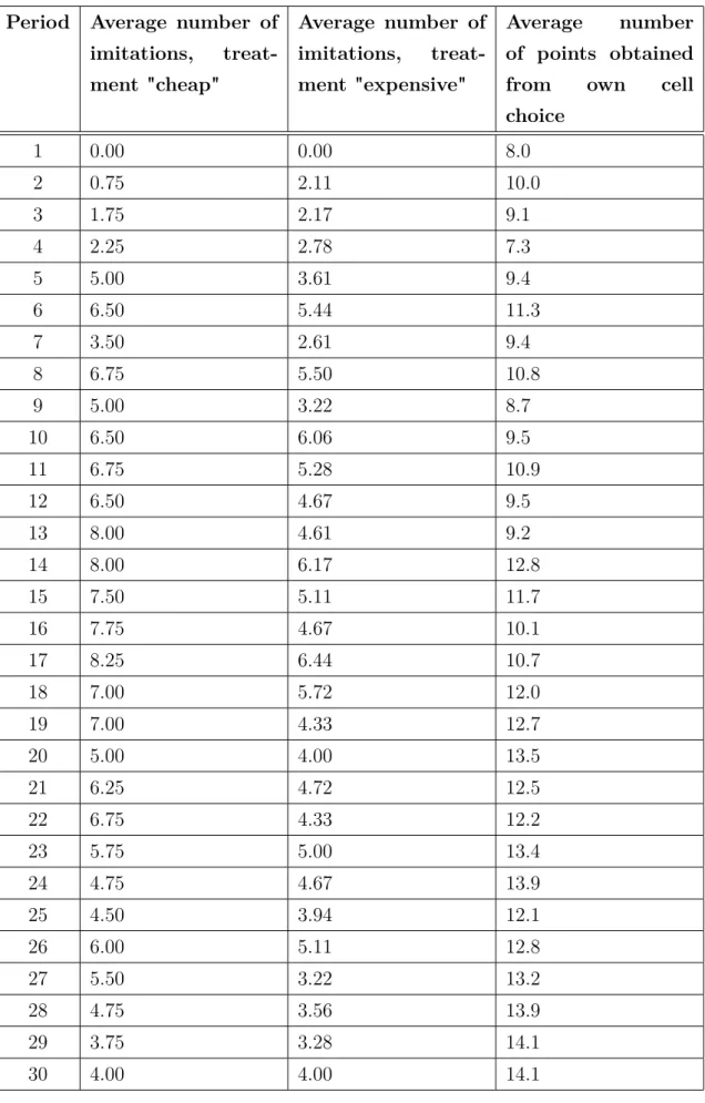
The experiment described in this chapter analyzes the behavior of people in situations where imitation can help them avoid bad outcomes, but is not required for learning. Participants faced a simple task where they had to choose cells from a table. Each cell returned points, but which cell returned how many points changed according to a regular pattern. There were two types of participants: informed and uninformed, where the informed types knew more about the pattern of changes than the uninformed types. In addition to choosing cells themselves, players could also imitate other players by following their cell choice. They would then obtain the number of points that the imitated player obtained, minus a fee.
The experiment is designed to mimic market situations where some players are better informed than others, but no one can learn anything through imitation that he could not learn by pure observation. The results show that players imitate to a significant degree, and do so intentionally. They start imitating once they have found out whom they should imitate, i.e., which players receive high numbers of points. They stop imitating once they have learnt the pattern of changes themselves. When choosing a player to imitate, they do not only consider the points of the last period, but of at least four periods prior to the decision. This means that only if a player has high outcomes over several periods do the other players believe that the risk of bad outcomes is low when imitating him.
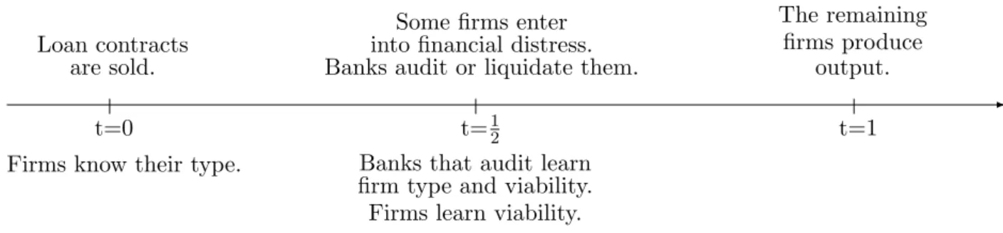
Finally, in the fourth chapter I analyze how the risk involved in lending offers private banks the chance to enter a market that would otherwise be dominated by a public (i.e., state-owned) bank. I consider the situation where there is an incumbent public bank that holds a state guarantee on its deposits, and a number of private banks that want to enter the market but face higher funding costs than the public bank. The public bank has the mandate to support the economy, while private banks are unrestricted in setting their policies. The borrowing firms have a certain risk of entering into financial distress during
the duration of the loan. There are two types of firms in the market: safe firms with a low probability of distress, and risky firms with a higher probability of distress. Some of the firms that are in distress are viable and produce output if their loan is extended. The rest of the distressed firms is unable to recover and produce output, such that extending their loans is inefficient.
I show that private banks can credibly commit to liquidating all borrowers in financial distress, and separate the borrower pool by offering a lower interest rate than the public bank. They can successfully enter the market and obtain positive profits in equilibrium. This strategy does not require that the public bank has the true objective to support the economic development. It suffices that firms have the perception that they will not be liquidated by the public bank at the onset of financial distress.
The mandate of the public bank helps private banks to overcome the competitive disad-vantage of higher funding costs. However, the entry of the private banks, which would be expected to increase competition, may lead to higher interest rates for all firms.
I thank Dorothea Kübler for valuable comments and advice, and Franz Hubert for insightful comments and for patiently listening to all my ideas - the reasonable ones and the not so reasonable ones. The essays in this thesis also benefitted from the comments of participants in seminars at Humboldt-Universität zu Berlin, Technische Universität Berlin, Wissenschaftszentrum Berlin and UC Berkeley, as well as participants of many conferences, work shops and summerschools, e.g., the 21st Annual Congress of the Eu-ropean Economic Association, the Verein für Socialpolitik Annual Meeting 2006, the IAREP/SABE Congress 2006, the International Workshop on Behavioral Game Theory and Experiments 2006 in Capua, and the 14th International Congress of the International Economic Association.
Last but not least I want to thank my boyfriend and my family for being the most lively discussants of my ideas and the pilot subjects of my experiments, and for making my life the pleasure it is.
Getting Used to Expectations
2.1
Introduction
Feeling disappointed when expectations change for the worse and delighted when they change for the better are emotions that are well known to most people. However, they cannot be explained with the existing models in either expected utility theory or behav-ioral economics. In this paper I introduce a novel concept, adjustment utility, which can explain the observed preferences, and yields new predictions for consumer behavior.
Consider the following two situations. In the first situation, Ms. Smith learns on Friday, February 4, that she will receive a wage increase in April, which she did not expect. However, on Monday, February 7, she learns that Payroll made a mistake and she will not receive this wage increase. In April she receives her usual wage. In the second situation, Ms. Smith is not told anything about a wage increase in February and receives her usual wage in April. In which situation is Ms. Smith happier on Monday, February 7?1
According to expected utility theory and behavioral economics, she is equally happy in both situations. She expects the same future outcomes, and the time until their realization is long enough such that the reference state for her wage in April can adjust to her expectations. However, most people would expect Ms. Smith to be happier on Monday if she were never told about the wage increase. In a classroom survey with 47 students, 44 (>90%) expected Ms. Smith to be happier in the second situation.2 This means that
past expectations have an influence on current utility from expectations, i.e., preferences 1Assume that she does not undertake consumption during the weekend which she would not have done
without the wage increase.
2I conducted this survey in January 2006 with participants of a Master course in Game Theory at
the Technical University Berlin. Most of the students in the course study industrial engineering. One student expected Ms. Smith to be happier in the first situation, for two she was equally happy in both. See the translated questionnaire in appendix B for details.
are path-dependent with respect to expectations. The state of Ms. Smith’s expectations over the weekend influences the utility she derives from her expectations on Monday.
I account for such preferences by introducing reference-dependent utility from expected future outcomes. Since this component of utility is caused by the adjustment of expec-tations, I term it adjustment utility. It explains individual behavior like that observed in the survey.
The model focuses on situations where the formation of expectations over future out-comes and the actual realization of those outout-comes are temporally separated. This applies, first, to situations in which people form expectations over a consumption decision prior to the actual decision. For example, people form expectations over the purchase of sea-sonal goods like summer shoes prior to actually buying them, and over the consumption of goods bought in catalogues prior to actually receiving them. Second, it applies to situations in which the consumption of the asset takes place prior to the realization of outcomes. This includes assets and actions whose consumption causes future health risks, like the risk of an HIV infection through unsafe sex, or the risk of adverse health effects from eating genetically-modified food. It also includes assets and actions which cause delayed benefits, like consuming healthy food and exercising.
The survey shows that past changes in expectations are relevant for current utility, which means that adjusting expectations is not utility-neutral. This implies that the ref-erence state for expectations can never be fully endogenized. The reason is that for any economically relevant asset, there is at least one moment in which the individual’s expec-tation regarding the asset changes. Even in the case of immediate full information that remains the same until final consumption, expectations change from initial unawareness to awareness of the future acts of consumption. After information is received, during the adjustment of the reference state from past to current expectations, the reference state is (partly) exogenous, since initial unawareness is exogenous.
Regarding the formation of the reference state, the survey shows the relevance of one’s own expected future state. A second survey shows a similar influence of the social comparison component. I again asked students to evaluate two situations. In the first situation, Ms. Smith is head of a department at her company and knows already in August 2006 that she will earn 50.000 EUR in 2007. She expects the other heads of department at her company to earn 40.000 EUR on average. On October 1, she learns that the other heads will also earn 50.000 EUR on average. In the second situation, she expects the other heads of department to earn 60.000 EUR on average, but then also learns that they will earn 50.000 EUR. In which situation is Ms. Smith happier on October 1? Again, according to received theory, there is no difference in her utility, since she expects the same future outcomes and her reference state has plenty of time to adjust to her expectations
until outcomes are realized. However, in the survey 61 out of 78 students (78%) expected Ms. Smith to be happier in the second situation.3
These results allow me to qualitatively specify the reference state for expectations to depend positively on the individual’s past expectations regarding her own future state, and her expectations regarding the future state of other members of her reference group.4 Even though these two qualitative relations do not characterize the reference formation process in as much detail as one would hope, they are all one can take from the surveys. They are also sufficient to derive results on people’s utility, and their behavior towards assets and actions that induce future outcomes.
To derive the model’s predictions, I analyze the equilibrium strategies in the spirit of the personal equilibrium that Koszegi and Rabin (2006) derive for realized outcomes. It is shown that when considering adjustment utility, an individual’s strategy can in equi-librium lead to choices opposite to those that would obtain in the personal equiequi-librium without adjustment utility. In particular, in situations where the individual would have chosen not to consume a certain asset in the personal equilibrium without utility from ex-pectations, with adjustment utility it may be her unique equilibrium strategy to consume the asset.
In general, reference formation regarding expectations leads to a change in the utility from assets that induce outcomes in the future, even if no change in the parameters of the assets occurs. For example, people are less frightened by the risk of adverse health effects from genetically-modified food once they get used to consuming such food, i.e., once their reference state adjusts towards the effects that may result from its consumption. As a result, sophisticated individuals who are able to predict their future reference states derive higher utility from consuming an asset that induces negative expected outcomes than naive individuals who are unable to predict their reference states. For both types of individuals, there evolves a tendency of increased risk acceptance in the population without a change in the exogenous parameters.
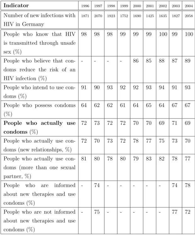
People getting used to their expectations and forming reference states regarding them offers an explanation, e.g., for the increasing acceptance of the risk of an HIV infection in Germany since the late 1990s. The data shows that people are at least as well in-formed about the risk of an HIV infection and the protective effect of condoms as before.5
3The survey was conducted at the Technical University Berlin in May 2006. Again, most of the
students are industrial engineers. No student participated in both surveys. Note that it cannot be determined for either survey whether the students interpreted Ms. Smith to believe in the information or her expectation to 100% or less. This does not, however, effect the argument.
4I define the reference group of an individual endogenously as the group of people who’s utility is
affected by the choices of this individual, and who’s choices affect the utility of the individual.
However, the use of condoms has decreased slightly but significantly between 1997 and 2004, which provides one reason for the increase in HIV infections in recent years. Since the data show that lack of care due to the availability of new therapies cannot explain this effect, gradual reference point adjustment towards the risk of an infection offers a plausible explanation. Over several years, people may have themselves accepted the risk of an infection occasionally and have learnt of others accepting the risk, e.g., through the media. This means that the risk has - to a small but significant degree - been included in people’s reference states. Accordingly, the disutility from accepting the risk has decreased (the utility has increased). This means that less (non-monetary) costs are accepted in order to avoid the risk, leading to a decrease in the use of condoms.
In addition to explaining observed preferences and attitudes towards risks, the model yields implications for policy. It shows that the release of positive but dubious information may decrease welfare. Contrary to existing models, when accounting for adjustment utility, the release and subsequent correction of positive information may lead to negative net utility. This is the case if the initial delight after the release of the information is overcompensated by the disappointment caused by the correction. The more loss averse individuals are, the more likely is a negative overall effect.
Further, if regulatory measures of newly introduced assets that involve future health or environmental risks are based on current rate of consumption estimations without account-ing for changes in the reference state, they will underestimate the extent of consumption in the medium to long-term. Accordingly, either will production and consumption of the asset exceed the socially optimal level, or regulation will have to be adapted later on, which may be costly and/or hard to implement.
In section 2.2, I briefly describe reference-dependent preferences and utility from ex-pectations. The concept of adjustment utility, the definition of the reference state for expectations, and the expectation personal equilibrium are developed in section 2.3. I derive the change in utility that an individual experiences when repeatedly consuming a risky asset in section 2.4. The individual’s choice between the risky and a comparable safe asset is analyzed in the context of her overall consumption optimization in section 2.5. Section 2.6 derives the value of information, while section 2.7 shows that the reference state cannot be endogenized in general. Finally, section 2.8 derives further implications and concludes.
2.2
Reference-dependent preferences and utility from
expectations
Consider an asset which induces a set of outcomes x ∈ X with distribution function
f(x) some time after consumption.6 The asset is consumed in period t and outcomes
are realized in period T, with T > t. The asset may also induce outcomes immediately upon consumption, but since they are not relevant for the analysis, they are normalized to zero.7 Where no confusion can arise, I will abbreviate the asset with F.
Individuals derive reference-dependent utility from the outcomes induced by asset F. Utility inT consists of the reference-independent part ux(x), and the reference-dependent part vx(x|rx) with rx as the reference state for realized outcomes.8 I will call the utility Ux that the individual derives from the realization of xoutcome utility: Ux(x) =ux(x) +
vx(x|rx).
The reference-dependent outcome utility fulfills Kahneman and Tversky (1979) con-ditions for the relative value function, i.e., v(x|r) is defined as a finitely valued function
v :X×X →R, and
A1: v(x|x) = 0 for all x.
A2: v(x|rx) is continuous for all x and twice differentiable forx6=rx;
A3: v0(x|rx)>0 for all x given rx.
v(x|rx) is to be interpreted as a measure of the value of x relative to rx when both are viewed from the reference point rx. In any period s < T, the individual then expects the utility Ux(f(x), rx) = ux(f(x)) +vx(f(x)|rx) to be experienced in period T, with rx as the expected reference state for outcomes in T.
There exists both experimental and empirical evidence for the reference dependence of individuals’ outcome utility. It shows that the majority of people evaluate outcomes relative to a reference point in many spheres of utility, e.g., for consumption levels and wages (see, e.g., Kahneman et al. (1991), for experiments on the endowment effect, or Benartzi and Thaler (1993), for an explanation of the equity premium puzzle for loss averse investors).
However, individuals do not only derive outcome utility from the consumption of asset
F. Rather, from expectingf(x) to be realized inT they derive utility in each periodswith
t ≤s < T, i.e., in each period between the consumption of asset F and just prior to the realization of outcomes. Utility from expectations is experienced whenever an individual
6The degenerate lottery withf(x
0) = 1 for a certain outcomex0is included.
7Since I do not consider preference reversals over time here, e.g., quasi-hyperbolic discounting, having
non-monetary outcomes at two moments in time would not add to the analysis.
looks forward to expected future events (see, e.g., Loewenstein (1987) for the utility from anxiety and pleasant anticipation). In an economic context, utility from expectations has been considered by, e.g., Caplin and Leahy (2001), Koszegi (2005) and Brunnermeier and Parker (95). There, anticipatory utility reflects the reference-independent utility people derive from expecting future outcomes. These models show that anticipatory feelings influence economic behavior and are relevant for utility.
I define the anticipatory utility that is experienced in all periods s with t ≤ s < T
as uas = uas(f(x), rx), i.e., it depends on the utility individuals expect to experience in
T. Accordingly, it depends on the outcome distribution and the reference state they expect inT. ua(f(x), rx) is assumed to be increasing inf(x), decreasing inrx, continuous and twice differentiable in both dimensions. For simplicity, I assume that ua(f(x), rx)> 0 ⇔ Ux(f(x), rx) > 0 and ua(f(x), rx) < 0 ⇔ Ux(f(x), rx) < 0, i.e., assets which induce negative expected utility also induce negative anticipatory utility, while assets which induce positive expected utility induce positive anticipatory utility.
Combining the concepts of reference dependence and anticipatory utility then yields the expected utility from consuming asset F as
ˆ U(f(x)) = T−1 X s=t uas(f(x), rx) +ux(f(x)) +vx(f(x)|rx) (2.1) where anticipatory utility ua is experienced in each period t≤s < T and outcome utility
ux+vx is experienced only in T. For simplicity, the discount factor is set to δ= 1. An alternative scenario to the one considered here is where the individual in period t
only expects to consume asset F inT, instead of consuming it. Upon consumption in T, however, she experiences outcomes immediately. In this case, the delay is in consumption, rather than in the realization of outcomes.9 Formally, these two scenarios are identical
for the purposes of this model, and all the results hold for both cases. For reasons of expositional simplicity, I will frame the model only in terms of the first scenario.
2.3
Adjustment utility
2.3.1
Definition
Reference dependence and anticipatory utility are not always able to explain observed preferences. To see this, consider again the two situations in the first survey. Regarding anticipatory utility, Ms. Smith is expecting the same future wage in both situations, such 9This is the setting in which Koszegi and Rabin (2006) develop their model of reference-dependent
that the same utility results.10 Regarding reference-dependent outcome utility, in the
first situation she expects a higher wage between Friday and Sunday, but then expects the lower wage from Monday onward. Reference-dependent outcome utility would only yield a difference in utility if these three days in early February had a lasting effect on Ms. Smith’ reference state in April. This seems implausible. It also contrasts with the literature. For example, if expectations form the reference state for outcome utility as in the model of Koszegi and Rabin (2006), one would expect that in the two months that remain until April Ms. Smith’ reference point for her wage has sufficient time to adjust to her wage expectation. Accordingly, she derives the same expected reference-dependent outcome utility from her wage in April as if she had always expected her usual wage.11
With reference dependent utility from expected outcomes, preferences as expressed in the survey can be explained. For simplicity, in the further analysis I will follow Koszegi and Rabin (2006) and assume that for all individuals E(rx) = E(x), i.e., all individuals assume that between periods t and T their reference point for outcomes in T adjusts to their expectations regarding those outcomes. This allows me to abstract from the dependence of the utility from expectations on the expected future reference staterx, i.e., to write ua(f(x)) rather than ua(f(x), rx).
Definition 1 Let f(x) denote a lottery over the set of possible outcomes X induced by asset F and f(x) the set of possible lotteries over X.
The adjustment utilitythat an individual derives from expecting lottery f(x)∈f(x) given her reference lottery ra ∈f(x)is defined as va(f(x)|ra), where va denotes a finitely valued
function va :f(x)×f(x)→R and A4: va(f(x)|f(x)) = 0 for all f(x).
A5: va(f(x)|ra) is continuous for all f(x) and twice differentiable for f(x)6=ra;
A6: va0(f(x)|ra)>0 for all f(x) given ra.
In analogy to Kahneman and Tversky’s (1978) value function, adjustment utilityva(f(x)|ra) is to be interpreted as a measure of the value of expecting lotteryf(x) relative to expect-ing the reference lottery ra, when both are viewed from the expectation of the reference lottery ra.
The utility from expecting the lottery implied by assetF then consists of anticipatory utility ua(f(x)) and adjustment utility va(f(x)|ra)12:
Ua(f(x)) =ua(f(x)) +va(f(x)|ra) .
10This also holds if anticipatory utility depends on expected future reference states, see the argument
below.
11A more detailed analysis of the argument that Ms. Smith simply fails to correctly predict her reference
state, which may seem to explain the data at first sight, is relegated to appendix C.
Adjustment utility captures the observation that the pleasure or pain people derive from expecting future outcomes depends on what they compare them to, not only on their absolute amount. If you expected a vacation in the Himalayas next summer, and then learn that you will only go to the Alps, you will initially derive different utility from anticipating this vacation than if you had expected to stay at home, even if you are aware that your reference state for outcome utility will adjust to the vacation in the Alps in both cases until next summer.
Instead of the utility in (2.1), the individual’s utility from consuming assetF is there-fore given as U(f(x)) = T−1 X s=t [uas(f(x)) +vsa(f(x)|ra)] +ux(f(x)) +vx(f(x)|rx). (2.2) Anticipatory utility ua(f(x)) and adjustment utility va(f(x)|ra) are experienced in all periods between the consumption of the asset and the period just prior to the realization of outcomes. When outcomes are realized, reference-independent outcome utility ux and reference-dependent outcome utilityvx are experienced. Note again the important differ-ence between the two referdiffer-ence states: rx is the individual’s reference for the outcomes she experiences in T, i.e., a reference outcome. ra is the reference for the expectations she experiences in all periods up to T −1, i.e., a referenceexpectation. E(rx) is the refer-ence outcome the individual predicts for T, while E(ra) is the reference expectation she predicts to have at some time prior to T. Even though there is probably a connection between the two, they are never relevant for experienced utility at the same time.
The sequence of events in each period is as follows. If there is new information regard-ing the asset it becomes available first. Then the person experiences utility (from either expected or realized outcomes, depending on the period) given the available information and her current reference state. Next she observes others’ behavior. Finally, her reference state for the next period is formed.
2.3.2
Reference state formation
From the surveys there emerge two factors that influence the reference state. The first is individuals’ past expectation of their own state: Ms. Smith’ expected April wage at the weekend influenced her reference wage expectation on Monday. The second is the expectation of others’ states: Ms. Smith’s expectation in September 2006 of her colleagues’ wages in 2007 influenced her reference expectation regarding their wages on October 1, 2006.
expected utility in T, which depends on rx. However, since I assumerx =E(x) throughout, I drop the
This parallels the findings for outcome utility. There the reference state has been found to be influenced by the individual’s own past consumption level, wage, investment return etc. (e.g., Kahneman et al. (1990), Campbell and Cochrane (1999) and by relevant others’ consumption levels, wages etc. (e.g., Abel (1990), Constantinides (1990).
The surveys do not, however, provide sufficient insight to infer a quantitative rela-tionship between these two factors, or even to quantify their influence on the reference state.13 Accordingly, I will not specify an explicit functional form of the reference state,
but limit the specification to qualitative relations. I also take account of the fact that events further in the past are less present in people’s minds than the same events in more recent periods. Accordingly, they must be expected to be less relevant for the formation of the reference state and will receive a "mental discount".
Let fi,t(x) denote the expectation person i has in period t of her own future state regarding asset F, andf−i,t(x) denote the set of expectations she has of the future states of the members of her reference group. β denotes the mental discount factor, which may differ across assets and individuals: 0 ≤ β ≤ 1. Considering a sequence of past expectations and weigthting it with a discount factor smoothes the reference formation process. It takes account of the fact that reference formation in most cases must be expected to be a gradual process. After a change in expectations, the reference state may take some time to adjust to the new situation. In contrast, considering only last period’s expectations would lead to jumps in the process, i.e., ad hoc adjustments of the reference state. In addition, through adjusting β properly, the process does not depend on the definition of the length of a period.
Another principle that I assume the reference formation process to observe is conver-gence. If expectations regarding one’s own future state and the states of relevant others are constant for a long time at fi and f−i, the reference state for adjustment utility con-verges towards a state that reflects only these expectations, i.e., towards the reference state that would result if it only depended on last period’s expectations fi and f−i.
Definition 2 The reference state for the adjustment utility of individual i in period t is defined as
rai,t =rai,tβt−s, fi,s(x),f−i,s(x) s<t (2.3) with ∂rai,t ∂fi,s(x) >0 and ∂r a i,t ∂f−i,s(x) >0 (2.4)
13This is, unfortunately, a problem this research shares with many others’ on the issue of reference
∂βt−s ∂s >0 and β1 = 1 ra(β,0,0) = 0 (2.5) limt−s→∞βt−s = 0 (2.6) limt−s→∞ rai,t βt−s, fi,f−i s<t =r a i,t fi,f−i (2.7) The term rai,t(βt−1−s, fi,s(x),f−i,s(x))s<t captures that the expectations of all periods prior to period t are taken into account, weighted with their respective discount factor. Note that (2.3) and (2.4) are applied to each line of the probability vector separately.
An example of a functional form of the reference state that complies with this definition is ri,ta =q X s<t βt−s P s<tβt−s fi,s(x) ! + (1−q) X s<t βt−s P s<tβt−s f−i,s(x) !
with 0< q <1 as the weighting factor for individual vs. social comparison. To illustrate the formation of the reference state, consider again the situations in the surveys. Equation (2.3) and the inequalities in (2.4) imply that the reference state to which an individual compares her wage expectation increases if she expects a higher wage and if others expect a higher wage. If no one ever expects to receive a wage, the individual’s reference state for her wage expectation is zero (equation (2.5)). Equation (2.6) captures the property that the wage expectations the individual and the members of her reference group had a long time ago have a negligible influence on her current reference state. Finally, with convergence (2.7), if the individual and relevant others expect the same wage for a long time, the individual’s reference state converges towards the reference state that would result if only last period’s wage expectations were considered.
2.3.3
Expectation Personal Equilibrium
In this section, I apply the concept of Koszegi (2005) personal equilibrium (PE) to the model of adjustment utility and consider the predictions this yields. Consider an individ-ual who has rational expectations and is aware of her reference formation process. At any time t, she forms expectations regarding the asset’s outcomes in T given her behavior in
t. From these expectations she can predict her future reference states rsa for all periods
t < s < T according to (2.3).14 Knowing her reference states she can derive her
adjust-ment utility. Considering all four components of the individual’s overall utility as defined in (2.2), she then chooses her optimal behavior int. If this behavior differs from what she assumed initially, it induces new expectations regarding her outcomes inT, her reference
state ra
s, her expected utility, and hence her (updated) optimal behavior. This process continues until it reaches a state where the behavior from which she derives her expecta-tions and the optimal behavior that result from them are identical. Depending on what behavior she assumed initially, this fixed point problem may yield several equilibria. It is similar to the optimization problem in Koszegi and Rabin (2006) for outcome utility. It includes two loops. The first one is the feedback loop from the individual’s behavior into her reference state and from her reference state into her behavior. This loop includes the (potentially) exogenousra and the subsequent reference formation process. The second is the social comparison feedback loop from the individual’s behavior to the reference state and behavior of others, and from the behavior of others back to the individual’s reference state and behavior. Solving the fixed point problem, therefore, requires the assumption of common knowledge of the reference formation process and utility of all members of the reference group. Even though this may seem demanding, it is common in the literature and useful in order to be able to compare my results with those of earlier models. It shows where the inclusion of adjustment utility yields novel predictions. I briefly consider the case when this assumption is violated, i.e., naivety, in the next paragraph.
Definition 3 Let ra(f(x)) and rx(f(x)) denote the reference states for adjustment util-ity and outcome utilutil-ity, respectively, that result from choosing the lottery f(x). A choice
f(x) ∈f(x) forms an expectation personal equilibrium if for all possible choices f0(x)∈
f(x) T−1 X s=t [ua(f(x)) +va(f(x)|ras(f(x)))] +ux(f(x)) +vx(f(x)|rx(f(x)))≥ T−1 X s=t [ua(f0(x)) +va(f0(x)|ras(f0(x)))] +ux(f0(x)) +vx(f0(x)|rx(f0(x)))
In words, an individual’s choice forms an expectation personal equilibrium if, given her reference state for adjustment utility and the reference formation process of her as well as of others given this choice, she derives utility from this choice which is at least as high as that derived from any other possible choice and the reference formation processes that result from this choice.
When does an expectation PE yield predictions different from Koszegi and Rabin (2006) outcome PE? For ease of comparison, consider their example of a shoe purchase. Assume that an individual is used to buying new shoes in spring. Towards the end of winter, she receives the catalogue for shoes that will be available in spring. But this year she realizes from studying the catalogue that shoe prices have increased and new shoes may be beyond her means. Assume that if the individual considers only outcome utility,
it is her unique outcome personal equilibrium strategy not to buy the shoes in spring. She makes this decision predicting that her reference state for the purchase will adjust to her expectation of not buying the shoes until spring actually comes, such that not buying shoes is not felt as a loss then. Now add the utility from expectations. First, taking into account anticipatory utility makes the purchase of the shoes more attractive, since the individual can look forward to the purchase and derive utility from that. Second, and more important here, including adjustment utility makes the purchase of the shoes more attractive since it avoids the disappointment the individual would experience from adjusting her expectations towards expecting not to buy the shoes since she initially expected - without detailed knowledge of the market - to buy shoes as every year. Her reference state in winter, which included the expectation to buy shoes in spring, makes the expectation of not buying the shoes be felt as a loss. This is different from the utility in spring, for which the individual has time to get used to the idea of not buying the shoes and may not feel disappointed. In summary, if the reference state in winter is the expectation to buy the shoes, e.g., because the individual is used to buying shoes in spring, adjustment utility increases the utility from buying the shoes. This means that there exist cases where it is the individual’s unique strategy in Kőszegi and Rabin’s outcome personal equilibrium not to purchase the shoes, but her unique strategy in the expectation personal equilibrium to purchase the shoes.
Proposition 1 Consider an individual who has the choice between f(x) ∈ f(x) and
f0(x)∈f(x). Then, if T−1 X s=t [va(f(x)|rsa(f(x)))−va(f0(x)|rsa(f0(x)))]< T−1 X s=t [ua(f0(x))−ua(f(x))] +ux(f0(x))−ux(f(x)) +vx(f0(x)|rx(f0(x))−vx(f(x)|rx(f(x)))
the individual’s strategy in expectation personal equilibrium is f0(x), while the strategy in outcome personal equilibrium is f(x).
Proposition 1 results directly from the definition of an expectation PE. It shows that if the difference in aggregated adjustment utility between two choices is larger than the difference in anticipatory and outcome utility and of the opposite sign, the choice predicted by the expectation PE is opposite to the one predicted by the outcome PE, even if one accounts for anticipatory utility in both equilibria.
2.3.4
Naivety vs. Sophistication
An individual that is aware of her reference formation process knows that the decision to consume the asset F involves a change in her reference state for expectations, which
induces a change in utility. When assessing the utility she derives from the consumption of the asset, she takes account of this effect. In particular, if she consumes an asset which induces negative expected future utility, she knows that her reference state will decrease and she will derive higher utility from expecting the asset’s outcomes in the periods up to their realization. Similarly, if she consumes an asset which induces positive expected future utility, she knows that her reference state will increase and she will derive lower utility from expecting the asset’s outcomes.
An individual that is not aware of her reference formation process does not predict the effect of the reference point change on her utility and hence assumes that she will experience the same utility in each period up to T.
Accordingly, a sophisticated individual assigns a higher overall utility to the consumption of an asset with negative expected future utility than a naive individual, but a lower overall utility to an asset with positive expected future utility.
2.4
Repeated consumption
So far I have analyzed the consumption of the asset only in one period. In this section, I derive the change in the individual’s net utility from asset F when she considers its consumption repeatedly. I begin in section 2.4.1 with analyzing the utility of consuming
F at different stages of the reference formation process. For the same reference formation process, in section 2.4.2 I derive the utility of not consuming F, i.e., the utility of not expecting its future outcomes. The comparison of the two utilities shows the change in the attraction of F when the reference state changes.
Finally, rather than analyzing F in isolation as in sections 2.3 and 2.4, in section 2.5 I introduce prices and extend the analysis to the individual’s overall consumption optimization. In addition toF, the individual can now choose to consume an alternative asset, which does not induce future outcomes but differs from F in its price. This means that since the choice of F also influences the individual’s ability to consume other goods, her reference state for these goods has to be taken into account. This finally allows me to derive the individual’s decision regardingF from her overall consumption optimization program.
2.4.1
Utility of consuming the asset
Consider now the repeated consumption of asset F. For example, an individual may repeatedly eat genetically-modified food and after a while get used to expecting possible adverse health effects from this in the future. I analyze utility starting in period t, where
t is the period such that before period t no member of the reference group has ever consumed the asset, but in t at least one individual consumes it. However, the argument that is developed below holds for all situations whererahas not yet fully converged to the state that reflects permanent consumption of F by all members of the reference group.
The results of the previous sections were derived assuming only that people’s prefer-ences were reference-dependent and decreasing in the reference state. In order to obtain quantitative results, I now add the assumption that individuals are loss averse for both realized and expected outcomes, i.e., their relative value function for realized outcomes and their adjustment utility function are steeper for losses than for gains.
Compare the individual’s utility from consuming the asset for the first time in period
t to consuming it the second time in period t+ 1. If consumed in t the asset induces outcomes in T, while if consumed in t+ 1, it induces outcomes in T + 1. I do not allow for any new information regarding the asset to become available in t+ 1, i.e., I keepf(x) constant. This means thatua
s(f(x)),ux(f(x)) and vx(f(x)|rx) are constant in all periods untilT + 1.
Note that, in order to account for the accumulation of expected outcomes, rsa now explicitly refers to all relevant expected outcomes of asset F. Considering only decisions in period t and t+ 1, this includes outcomes in T and T + 1. The number of outcomes could, however, be extended to include any number of relevant expectations. Formally, this means that15
ri,ta =ri,ta (βt−s, fi,s(xT),f−i,s(xT), fi,s(xT+1),f−i,s(xT+1))s<t and rai,t+1 =rai,t+1(βt+1−s, fi,s(xT),f−i,s(xT), fi,s(xT+1),f−i,s(xT+1))s<t+1 .
Consider the individual in isolation first, i.e., ignore the effects of social comparison. For simplicity, and since it would not add any new insights, I again abstract from discounting (δ= 1). Since I only deal with one individual here, I drop the index i. The difference in utility is then given as
Ut+1(f(x))−Ut(f(x)) = T X s=t+1 [uas(f(x)) +vsa(f(x)|rsa)] +uxT+1(f(x)) +vTx+1(f(x)|rx) − T−1 X s=t [uas(f(x)) +vsa(f(x)|rsa)]−uxT(f(x))−vTx(f(x)|rx) .
Since ux(f(x)) and vx(f(x)|rx) are the same in T and T + 1, ux
T +vTx and uxT+1 +vTx+1
offset each other:
Ut+1(f(x))−Ut(f(x)) = T X s=t+1 [uas(f(x)) +vsa(f(x)|rsa)]− T−1 X s=t [uas(f(x)) +vsa(f(x)|ras)] .
15For the general case when n periods are considered, this extends to ra i,t =
ra
i,t(βt−s,Pnfi,s(xT+n),Pnf−i,s(xT+n)))s<t where the interval [T, T + n] includes all periods
Both terms above contain (T −t −1) terms ua
s(f(x)) , which, given that uas(f(x)) is constant in all periods, is the same such that
Ut+1(f(x))−Ut(f(x)) = T X s=t+1 vas(f(x)|ras)− T−1 X s=t vsa(f(x)|rsa) .
Since ras is relevant for all assets in period s, i.e., the reference state is the same for all assets F, reference-dependent anticipatory utilities of the two assets between t+ 1 and
T −1 drop out, yielding that
Ut+1(f(x))−Ut(f(x)) = vTa(f(x)|r a T)−v a t(f(x)|r a t) .
The individual did not consume asset F before t. Hence, f(x)s<t = 0 and, abstracting from social comparison effects,ra
s≤t=0.
16 After consuming the asset in t,f(x)
t≤s<T 6=0 and ra adjusts towards f(x) according to (2.3). The more time between t and s, i.e., the further the reference formation process has proceeded, the further away from zero is
ra, since for β < 1 the weight of f(x)s<t = 0 decreases while the weight of f(x)s≥t 6= 0 increases.
Hence, if the individual consumes the asset repeatedly, her ra decreases over time if the asset induces negative expectations and increases if it induces positive expectations. This means that:
Ut+1(f(x)) > Ut(f(x)) if f(x)≺0
Ut+1(f(x)) < Ut(f(x)) if f(x)0 . with the initial reference statera=0. In general,U
t+1(f(x))> Ut(f(x)) iff(x)≺ra and
Ut+1(f(x))< Ut(f(x)) if f(x)ra.
Consider now the process for individuals with social comparison preferences, where
f−·(x) denotes the expectations of the respective individual regarding the outcomes of all
individuals of her reference group. As before, rat =0 at time t for all individuals in the reference group, and at least one individual consumes F in t. This leads to ra
t+1 ≺ rat if the asset induces f(x) ≺0 and ra
t+1 rat if it induces f(x) 0 for all individuals in the group. Since for all individuals f−·(x) 6= 0 in all periods up to T −1, rTa 6= rta = 0, i.e. ra
T ≺rta if f−·(x)≺ 0 and raT rat if f−·(x)0, for all individuals in the reference group.
Then, if an individual considers consuming F in t+ 1, independently of the predicted future behavior of herself and relevant others, it results that
Ut+1(f(x)) > Ut(f(x)) if f(x)≺0
Ut+1(f(x)) < Ut(f(x)) if f(x)0
for all individuals in the reference group. These results are summarized in 16Sincef(x) andra are vectors,0denotes the zero vector.
Proposition 2 Consider an individual that in period t starts consuming an asset which induces future expected outcomes. The utility that this individual and the other members of her reference group derive from consuming the asset in period t + 1 increases if the asset induces negative expected utility, but decreases if it induces positive expected utility.
For example, the utility people derive from consuming genetically modified food in-creases the more often they consume it. In contrast, the utility they derive from organic food decreases the more they get used to it.
2.4.2
Utility of not consuming the asset
For the decision of whether to consume the asset or not, the effect of reference state formation on the alternative utility of not consuming the asset is equally important, since eventually the difference in utility is decisive. This utility is affected by ra in the same way as is the utility of consuming the asset. Consider an asset which induces negative expected future outcomes, f(x) ≺ 0. The utility of not consuming the asset increases if it was consumed in the past, since with a lower ra a utility of zero feels like a higher gain. Starting from ra
t = 0, a marginal reference point change to rta+1 ≺ 0
leads to a state where not consuming the asset is felt as a gain (from neither gain nor loss for ra
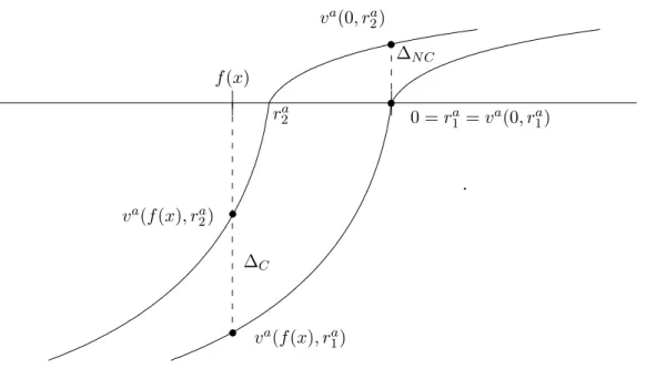
t = 0) and the consumption of the asset is felt as a marginally smaller loss. Considering the entire reference formation process, for loss averse individuals a change in the reference point from ra = 0 to ra = f(x) ≺ 0 leads to a higher increase in the utility of consuming the asset (∆C =va(f(x)|r2a)−va(f(x)|ra1) than in the utility of not
consuming it (∆N C =va(0|r2a)−va(0|r1a), see figure 2.1). Hence, the consumption of the
asset becomes more attractive.17
For assets which yield positive expected outcomes, e.g., health benefits from exercising, healthy lifestyle etc., the utility of not consuming the asset decreases with an increasing reference point, and since it is felt as a loss, for loss averse individuals it decreases faster initially than the utility of consuming F. Accordingly, the relative utility of consuming the asset compared to not consuming the asset increases. Hence, even though section 2.4.1 showed that the utility from the asset decreases, consuming the asset nevertheless becomes more attractive relative to not consuming it.18
17Note that if f(x) causes large losses, the initial increase in utility of not consuming the asset may
exceed the increase for the consumption of the asset. This is the case if va at 0 > ra is steeper than
at f(x)< ra. Then, for a certain part of the reference formation process, the consumption of the asset becomes relatively less attractive after a decrease inra.
18Only if the final loss that is derived from an expectation of zero, given a reference pointra=f(x)0,
is large, the utility from consuming the asset may temporally decrease faster for an increase in the reference state than that from not consuming the asset.
.. f(x) ra 2 va(f(x), ra 1) va(f(x), ra 2) 0 =ra 1 =va(0, r1a) va(0, ra 2) ∆C ∆NC 1
Figure 2.1: Effect of reference state change with f(x)≺0
If the reference lottery moves fromra1 tora2, the adjustment utility of the degenerate lottery that
yields zero in all states (no consumption of F) increases from 0 to va(0, ra2). The adjustment
utility of the lottery f(x) induced by the consumption of assetF increases fromva(f(x), r1a) to va(f(x), ra2). With va steeper for losses than for gains, the net effect is an increase in utility
from f(x) relative to the zero lottery.
2.5
Consumption optimization
2.5.1
General case
As the final step of the analysis I now add prices, and take into consideration the individ-ual’s reference formation regarding her overall consumption. I compare her utility from consuming asset F with that of consuming an alternative asset which induces the same current utility as F but no future outcomes. For ease of exposition, I restrict the analysis to assets F which yield negative expected outcomes, i.e., "risks". In addition, I focus on assets that induce non-monetary outcomes like health effects. This allows me to simplify the analysis by assuming that monetary and non-monetary utility are separable.
In period t, the individual receives monetary income Yt and can choose between the risky assetF and the alternative safe assetS, which yields the same outcomes at present but no outcomes in T. I normalize present outcomes of assets F and S to zero.19 The
price for the safe asset S is normalized to PS := 0. The risky asset F has a discount 19Since present outcomes are the same, reference point effects for those outcomes are also the same
π, such that PF = −π. For example, the individual has the choice between consuming genetically-modified food and organic food, where organic food is safe but more expensive (and I assume that both taste the same at present).
ra(f(x)) as before denotes the reference state that results if F is consumed, while
ra(S) denotes the reference state that results if S is consumed, i.e., if there are neither bad nor good outcomes inT. In addition toF andS, individuals can invest into monetary consumptionct, and utility from monetary consumption is denoted withUc. To keep the model simple, I abstract from savings, which means that monetary consumption in periods
s > t has no influence on the optimization.20
Let the parameter ξ denote the decision, where ξ = 0 if the safe asset is consumed and ξ = 1 if the risky asset is consumed. The individual’s optimization problem is then given by maxξ Uc(ct) + ξ "T−1 X s=t (uas(f(x)) +vsa(f(x)|ras(x))) +uT(f(x)) +vT(f(x)|rx) # + (1−ξ) T−1 X s=t [uas(S) +vsa(S|rsa(S))] s.t. ct = Yt+ξπ .
This yields the first order condition
U0(Yt+ξπ)π = T−1
X t
[uas(S) +vsa(S|ras(S))−uas(f(x))−vas(f(x)|ras(x))]−uT(f(x))−vT(f(x)|rx) Since S is safe, i.e., it does not induce health effects in the future, uT(S) = vT(S|rx) =
ua(S) = 0, where I use the fact that if the individual does not consume the asset, she expects no health effect, i.e., rx= 0. However, ua(S) = 0 is considered a gain forra <0, in which case va(S|ra(S))>0. I then obtain for the optimum that
U0(Yt+ξπ)π = T−1
X t
[vsa(S|ras(S))−uas(f(x))−vas(f(x)|ras(x))]−ux(f(x))−vx(f(x)|rx) In words, the risky asset F is preferred over the safe asset S if the utility increase due to the lower price of F exceeds the utility decrease due to the lower utility from expectations and realized outcomes caused by a possible adverse outcome inT. Note that this general trade-off is not affected by introducing saving opportunities into the model.
20This simplification does not affect the main results of the model, since I assume utility from
mon-etary and non-monmon-etary assets to be separable. This is common in the literature and seems at least a good approximation(see, e.g., Feldman and Dowd, 1991, who assume separability between medical care consumption and non-medical care consumption).
2.5.2
Indivisible assets
To keep the analysis tractable, I now limit it to assets that are indivisible, ξ ∈ {0,1}. This means that asset F can be consumed or not, but cannot be partly consumed. This applies, e.g., to decisions like whether to eat gm-food or not, practice safe or unsafe sex etc. I account explicitly for reference effects regarding consumption of monetary goods,
ct. In contrast to the non-monetary outcomes induced byf(x) (e.g., health effects), these are goods that can be bought, like food, clothing, cars etc. rc denotes the reference state for the outcome utility from these goods. Then, the risky asset is preferred over the safe asset if Uξ=1 > Uξ=0, i.e., iff:
uc(Yt+π) +vc(Yt+π|rc)−uc(Yt)−vc(Yt|rc) > T−1
X s=t
[vas(S|rsa(S))−uas(f(x))−vsa(f(x)|rsa(x))] − ux(f(x))−vx(f(x)|rx) (2.8) In this condition, expressions ra
s>t(f(x)), ras>t(S) and rx are endogenous, while rat and Yt are exogenous in t.
Consider first the influence of the reference formation process regarding adjustment util-ity on the optimization. The reference state ra only affects the term PT−1
s=t