UNBIASED BANDWIDTH ESTIMATION IN COMMUNICATION PROTOCOLS 1

UNBIASED BANDWIDTH ESTIMATION IN COMMUNICATION PROTOCOLS1 Krister Jacobsson∗_{Håkan Hjalmarsson}∗

Karl Henrik Johansson∗

{krister.jacobsson|hjalmars|kallej}@s3.kth.se

∗_{Department of Signals, Sensors and Systems, KTH,}

SE-100 44 Stockholm, Sweden

Abstract: Heterogeneous communication networks with their variety of application de-mands, uncertain time-varying traffic load, and mixture of wired and wireless links pose several challenging problem in modeling and control. In this paper we focus on bandwidth estimation and elucidate why estimates based directly on bandwidth samples are biased. Previously, this phenomenon has been observed but not properly explained, it seems. Standard techniques for bandwidth estimation are based on measurements of arrival times of packets as the bandwidth is proportional to the inverse of the inter-arrival time. Two main classes of bandwidth estimators are analyzed wrt how variations in the inter-arrival times affect the estimates. It is shown that linear time-invariant filtering of instantaneous bandwidth estimates does not change the bias. In contrast to this, smoothing the inter-arrival-time samples does give a bias reduction which depends on the properties of the smoothing filter. Hence, with such approach, noise attenuation can be traded against tracking ability wrt changes in the actual bandwidth.Copyright ©2005 IFAC

Keywords: Estimation, Communication Protocols, Communication Networks, TCP, Bandwidth

1. INTRODUCTION

Congestion control is one of the key components that has enabled the dramatic growth of the Internet. The original idea (Jacobson, 1988) was to adjust the trans-mission rate based on the loss probability. The first im-plementation of this mechanism, denoted TCP Tahoe, was later refined into TCP Reno. This algorithm (to-gether with some of its siblings) is now the dominating transport protocol on the Internet. The throughput and delay experienced by individual users are depending on several factors, including the TCP protocol, link capacity and competition from other users.

TCP is window-based which means that each sender has a window that determines how many packets in flight that are allowed at any given time. The

transmis-1 _{This work was supported by European Commission through the} project EURONGI, by Swedish Research Council and by SCINT.

sion rate is regulated by adjusting this window. For a network path with available bandwidthband RTTτ, the optimal window size isbτ, in the sense that if all users employed this window there would be no queues and the link capacities would be fully utilized. Using loss probability (as in TCP) to measure congestion means that the capacity of the network cannot be fully utilized. With necessity, queues have to build up (caus-ing increased delays) and queues have to overflow (causing loss of throughput). Several methods to cope with these short-comings have been suggested. In TCP Vegas (Brakmo and Peterson, 1995) a source tries to estimate the number of packets buffered along its path and regulates the transmission rate so that this number is low (typically equal to three). One interpretation of this algorithm is that it estimates the round-trip queu-ing delay and sets the rate proportional to the ratio of the round-trip propagation delay and the queuing

delay (Low et al., 2002). Both delays are obtained from measurements of the RTT.

Standard TCP protocols encounter difficulties when wired and wireless links are mixed, since packet loss and packet delays on wireless links may be interpreted as congestion by TCP. Several approaches to counter-act this problem has been suggested in the literature. Modifications of TCP has been proposed (Casetti et al., 2001; Sarolahtiet al., 2003). Other methods try to more directly differentiate loss as being either due to congestion or due to lossy wireless transmissions (Cen

et al., 2003; Samaraweera, 1999; Fu and Liew, 2003). Performance-enhancing proxies is an alternative in which either split connection schemes or

intercep-tion schemes are used (Elaarag, 2002; Mukthar et

al., 2003).

In a window based congestion control protocol with feedback, measurements of the returning packet dis-persion can be used to reconstruct the experienced throughput. This implicit information can be exploited and post processed into a suitable estimate for use in different congestion control applications. In the previously mentioned TCP clone Westwood (TCP-W) (Casetti et al., 2001) this is recognized, and throughput samples are used in the window recov-ery mechanism. The rationale is that the smoothed throughput is interpreted as the path available band-width and if a congestion event occur, the congestion window is set to match this rate instead of being dras-tically halved as in standard TCP. Avoiding getting too deep into the discussion if this available bandwidth is the fair share or not, we conclude that if the path available bandwidth (ABW) is defined as in (Jain and Dovrolis, 2003), i.e. the maximum rate that the path can provide to a flow, without reducing the rate of the rest of the traffic along that path, TCP-W should ideally strive towards its fair share and the protocol ob-jective seems reasonable. Nevertheless this demands a correct bandwidth estimate.

The Westwood scheme has shown good performance, especially in lossy network environments as wireless applications where packet losses mainly are due to link failure and not a signal of congestion (which is what TCP originally was designed for). However, de-spite good performance TCP-W interacts with other congestion control applications as its TCP siblings, and should hence be fair in the sense that if two com-peting flows are sending over the same link the steady state throughput should become equal. This issue has been investigated in e.g (Gerla et al., 2001; Grieco and Mascolo, 2002). In (Grieco and Mascolo, 2003) it is concluded that the original Westwood scheme over-estimate the available bandwidth in the pres-ence of ACK compression (Mogul, 1992) which ex-plains empirical problems with fairness towards less aggressive schemes. The observed phenomenon is at-tributed as aliasing effects, and to counteract this it is proposed that one should smooth suitable clusters of inter-arrival-times and then recreate the bandwidth

samples that are finally filtered. The bias in band-width estimation has also been observed in (Caponeet al., 2002). It is shown in simulation examples that the bias seems to disappear when the ACK inter-arrival-times are smoothed before the available bandwidth is calculated. Naturally the modified TCP scheme (TI-BET) is reported to be more friendly towards TCP Reno in wired networks.

In this contribution we elucidate on this issue and provide an, in our view, more lucid explanation of the phenomenon than the one given in (Grieco and Mascolo, 2003). The proposed model will also enable a rigorous analysis to the common empirical finding of (Grieco and Mascolo, 2003; Caponeet al., 2002) that smoothing the ACK inter-arrival-time attenuate the bias. We will provide an explicit expression for the bias as a function of the smoothing-filter. The analysis can be extended to the mean-square error of the bandwidth estimate (from which it follows that there is a trade-off between tracking ability, on one hand, and noise, and bias, attenuation on the other). Furthermore, as several new protocols employ adaptive filters both for bandwidth estimation, cf the original Westwood protocol (Casettiet al., 2001), and round-trip-time estimation, cf FAST (Jinet al., 2004), we will briefly discuss the static behavior of such filters. It will be shown that the mean static gain is typically biased compared to the corresponding time-invariant filter, and that the bias is heavily dependent on the traffic. This means that it may be difficult to ensure fairness for protocols employing such filters and that this quantity is very much dependent on the traffic conditions.

The outline of the paper is as follows. In Section 2 we discuss bandwidth estimation and explains why bias is present. As it has been recognized that e.g. TCP Westwood scheme suffers from this problem (Gerlaet al., 2001) we study the bias and the static properties of the original Westwood scheme in Section 3. In Section 4 we debate how to estimate the bandwidth so that the noise that the short-lived traffic induces does not introduce a bias in the estimate. Conclusions and future work are given in Section 5.

2. BANDWIDTH RECONSTRUCTION AND ESTIMATION

The throughput or average bandwidthbused by a con-nection is the successfully transferred amount of data normalized with the time interval in consideration. The average bandwidth can be reconstructed at the sender side by logging the ACK inter-arrival-time δi and the amount of corresponding acknowledged data

νiaccording to bn=∑ n i=1νi ∑n i=1δi (1)

Since we assume that the used bandwidth also is the fair share we will refer to it as available bandwidth in the sequel.

For stationary conditions on the path, i.e. constant cross-traffic load conditions, (1) is also the best es-timate of the available bandwidth at the time when packet n is ACKed. However, (1) is less suitable as estimate of the available bandwidth under varying load conditions. The reason being that the averaging in (1) makes it react slowly to changes in the available bandwidth. Considering the problem of processing (filtering) the inter-arrival-times into an estimate of the available bandwidth at the current time we are thus faced with two requirements. The estimate should

i) resemble (1) under stationary conditions, and ii) react quickly to changes.

In general these two requirements are conflicting thus enforcing a trade-off.

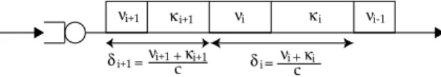
Consider the path bottleneck link with capacityc. This link is completely utilized by definition and outgoing packets travels back-to-back. If no interfering traffic is present downstream the bottleneck link or on the ACK path, the time space between two received ACK:s is the sum of the packet size νi and merging data

κi (deriving from competing flows) scaled by the

bottleneck capacityc, see Figure 1. Under stationary νi νi+1+ c κi+1 = δ i+1

νi+1 κ i+1 νi κ i νi-1

νi+

c

κi

=

δ i

Fig. 1. Packets traveling on the bottleneck link with capacitycMbps.

conditions, transmitting a constant packet sizeνi=ν, should ideally result in the merging traffic being of constant sizeκi=κ. This means that the inter-arrival-times would be perfectly evenly distributed, i.e.δi=δ for some constantδ >0, and hence, the instantaneous bandwidth estimate

ˆˆ

bi=ν_δi

i (2)

would equal the available bandwidthν/δ. However,

in practice, even with constant packet size νi=ν, the merging trafficκi is generally time varying. It is instructive to think of these variations as noise as these variations will average out over a longer time-interval. Packet displacements due to cross-traffic downstream the bottleneck, as well as ACK delays can also be considered as noise affecting the inter-arrival times. It is thus appropriate to introduce the model

δi=δi+ei (3)

where δi is the inter-arrival time that would be ob-tained when one packet of size νi is transmitted for each ACK and the load from cross-traffic is frozen at the present level and ideal conditions hold. As dis-cussed above, the noise term ei can be attributed to local variations in the cross-traffic at the bottleneck and the impact of cross-traffic downstream the bot-tleneck as well as on the ACKs. It seems reasonable to assume that when the cross-traffic is stationary,ei

can be modeled as a stationary stochastic process with zero mean.

Under this assumption the requirements i) and ii) above can be rephrased as that the bandwidth estimate should

• i’) reduce the impact ofei as much as possible, while still be able to

• ii’) track variations inδi.

Below we will analyze some approaches to this prob-lem.

2.1 Filtering the instantaneous bandwidth estimates

Viewing the instantaneous bandwidth estimates (2) as raw data, an obvious approach is to low-pass filter these estimates in order to obtain a smoother esti-mate. WithH(q) =∑∞k=0hkq−kdenoting a linear time-invariant (LTI) filter (hereq−1_{denotes the}

backward-shift operatorq−1_e

i=ei−1), the bandwidth estimate is

given by ˆ bb,n=H(q)bˆˆn= ∞

∑

k=0 hk ν_δn−k n−k (4)

Let us now analyze the impact of the noise ei un-der stationary conditions. Suppose therefore that the packet sizeνi=ν, a constant, so that δi=δ =ν/b wherebis the available bandwidth.

Under ideal conditions, i.e. whenen=0, ˆˆbn=ν/δis a perfect estimate of the available bandwidthb. Hence, in order to guarantee that the smoothed estimate ˆbn is unbiased, the filter should have static gain 1, i.e.

H(1) =1.

Now, notice that when the noise ei is non-zero, the instantaneous estimate is over-biased. The function

Φ(x) =ν/(δ+x) is convex and Jensen’s inequality

(Lehmann, 1983) implies Ehbˆˆn i =E[Φ(en)]>Φ(E[en]) =Φ(0) =ν δ =b (5) Hence, also the smoothed estimate is biased since

Eˆ bb,n=H(q) Ehbˆˆn i =Ehbˆˆn i >b (6)

where the second equality follows from thatH(1) =1. The bias can be quantified by expanding the raw bandwidth estimate (2) in a Taylor series

ˆˆ bn= ν δ+en = ν δ 1+ ∞

∑

j=1 (−1)je j n δj ! (7) Hence ˆ bb,n=H(q) ν δ 1+ ∞

∑

j=1 (−1)je j i δj !! =ν δ 1+ ∞

∑

j=1 (−1)jH(q)e j n δj ! (8)

and Eˆ bb,n=ν δ  1+ ∞

∑

j=1 (−1)jH(q)E h enj i δj   =ν δ 1+ ∞

∑

j=1 (−1)jmj δj ! (9) wheremjdenotes thejth moment E[enj]of the noise. Observe that the bias is independent on the properties of the filterH (as long as it has static gain 1) and is the same as for the raw bandwidth estimate ˆˆbn. We illustrate this in an example.

Example 2.1. Figure 2. shows outputs from different filters with bandwidth samples from a NS-2 simula-tion as input data. The dashed line is the bandwidth estimate produced by an arithmetic mean filter and the solid line is the bandwidth estimate produced from a first order filter with a pole at 0.99. The experimen-tal setup is a TCP SACK source sending data over a 5 Mbps bottleneck link. The congestion window bound and end-to-end delay are configured such that the link is completely utilized. At time 10 s a single UDP flow of 1 Mbps enters the bottleneck link. After the transient has died out we see that both filters reach the same level, and hence have the same bias.

6 7 8 9 10 11 12 13 14 15 4 4.2 4.4 4.6 4.8 5 5.2

Available bandwidth estimation

Time [sec]

Bandwidth [Mbps]

arithmetic mean, w = 100 westwood

exponential, α = 0.99

Fig. 2. Estimation by filtering directly on the width sample. Up to time 10 s the available band-width is 5 Mbps, after that 4 Mbps.

3. TCP-WESTWOOD

The original TCP-W scheme filters the instantaneous bandwidth samples and should, according to the anal-ysis in the previous section, be susceptible to bias. This has also been observed (Grieco and Mascolo, 2003; Caponeet al., 2002) and is also shown in Fig-ure 2 where the bandwidth estimate from the original time dynamic exponential filter in TCP-W (see (Gerla

et al., 2001)) is shown as the dotted line. Notice that, after the transient has died out, after the onset of the UDP-flow, this estimate doesnotreach the same level

as the arithmetic mean and first order filter estimates. This means that the bias for this estimate is different from that of a LTI filter. To better understand this we investigate the TCP-W filter in (Gerla et al., 2001), which is given by ˆ bw,n=αnbˆw,n−1+ (1−αn)dˆˆn with αn=2₂τ_τ−δn +δn, ˆˆ dn= ˆˆ bn+bˆˆn−1 2 (10)

whereτ is a filter parameter. The filter is thus linear, buttime-varyingand this is the reason for its different behavior. The estimate can be expressed as

ˆ bw,n= ∞

∑

k=0 (1−αn−k) k−1

∏

l=0αn−l ˆˆ dn−k (11) Notice first that ifαn=α, then the above is a first or-der filter with static gain 1. Now, in oror-der to get some intuition for this expression when the filter coefficients vary with time, let us, for the moment, use the simple model

αn=α+vn (12)

wherevnis modeled as a stationary stochastic process with zero mean. Assuming, for simplicity, that ˆˆbnand

vnare processes independent of each other gives that Eˆ bw,n=E "_∞

∑

k=0 (1−αn−k) k−1

∏

l=0αn−l # Ehbˆˆn−k i (13) >From this we see that when{vn}is an uncorrelated sequence, the filter has an average static gain 1 since all factors are independent with mean α. However, this will in general not hold when this sequence is correlated. We conclude that the bias in TCP-W will depend on the correlation of the filter coefficientsαn. Thus different scenarios will result in different bias. This is exemplified in Figure 3 where we apply a time varying first order exponential filter with correlated and uncorrelated coefficient sequences respectively to the experimental data just mentioned.

Returning to Figure 2 it can be observed that the the bias for the TCP-W estimate is less than the other two estimates in this scenario. From the above analysis it is clear that this is not an indication of superior performance of TCP-W in general as it is just a coincidence due to the particular correlation of the filter coefficients in this scenario. This have the effect that evaluating static fairness properties becomes a formidable task since the static fairness of a Westwood like protocol will depend on the composition of the cross-traffic at packet level.

4. UNBIASED AVAILABLE BANDWIDTH ESTIMATION

16 16.05 16.1 16.15 16.2 0.992 0.994 0.996 0.998 1 Time [sec] Bandwidth [Mbps] Filter coefficients

Filter 1: uncorrelated α sequence Filter 2: correlated α sequence

15.8 15.85 15.9 15.95 16 16.05 16.1 16.15 16.2 4.2 4.25 4.3 4.35 4.4 4.45 Time [sec] Bandwidth [Mbps] Bandwidth estimate Output filter 1 Output filter 2

Fig. 3. Coefficients and output of a time varying first order exponential filter with correlated and un-correlated filter coefficients.

bn=

1

n∑ni=1νi

1

n∑ni=1δi (14)

we see that we can interpret (1) as a way of smoothing (low-pass filtering) the variations in the inter-arrival time.

This suggests the general estimate ˆ

bt,n=F_H(q)(q)ν_δn

n (15)

In order to for this estimate to be unbiased under ideal conditions, the static gain of the LTI filtersF andH

should be unity.

We now analyze the bias of (15) under the same assumptions as in Subsection 2.1. We then have

ˆ bt,n=F_H(q)(q)ν_δn n = F(q)ν H(q)δ+H(q)en= ν δ+H(q)en (16) Comparing this with the instantaneous bandwidth es-timate (2) we see that the only difference is that en is replaced by the filtered noise H(q)en, hence the expansion equivalent to (7) is ˆ bt,n=ν δ 1+ ∞

∑

j=1 (−1)j(H(q)en) j δj ! (17) Thus, if the filter is such that the noise is attenuated, the inter-arrival-time smoothed estimate ˆbt,nwill have less bias than the raw bandwidth estimates ˆˆbn. Regarding the smoothed bandwidth estimate ˆbb,n, de-fined in (4), we see by comparing (9) with the mean of ˆ

bt,n, which from (17) is given by Eˆ bt,n=ν δ  1+ ∞

∑

j=1 (−1)jE h (H(q)en)j i δj  , (18)

that the filter H(q) does influence the bias of ˆbt,n. Hence, in contrast to what holds for ˆbb,n,H(q) can be used as a design variable (subject, of course, to

H(1) =1) to reduce the bias for the smoothed

inter-arrival-time based bandwidth estimate ˆbt,n.

We will illustrate this on a simplified example.

Example 4.1. Suppose thaten is an uncorrelated se-quence with variance λ◦ and that it is only the mo-ments up to order 2 that give a contribution to the raw bandwidth estimates ˆˆbn. For (2), it follows from (9) that Eˆ bb,n=ν δ 1+ ∞

∑

j=1 (−1)jmj δj ! =ν δ 1+λ◦ δ2 (19) which gives the bias

Eˆ bb,n−ν δ = ν δ λ◦ δ2 (20)

For the smoothed inter-arrival-time estimate ˆbt,n, sup-pose that H(q) in (15) is a first order filter with impulse response coefficientshk= (1−α)αk. Then, sinceenhas zero mean,

Eˆ bt,n=ν δ  1+ Eh(H(q)en)2 i δ2  = ν δ 1+ 1−α 1+αλ◦ δ2 !

which implies the bias Eˆ bt,n−ν δ = ν δ 1−α 1+αλ◦ δ2

Notice that the bias can be made arbitrarily small by choosingα sufficiently close to 1, i.e. by making the filter more and more low-pass.

We now illustrate the difference between smooth-ing raw bandwidth samples and smoothsmooth-ing raw inter-arrival-time samples by way of a NS-2 simulation.

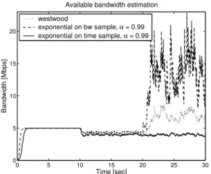
Example 4.2. The data originates from the same ex-perimental setup as before but with Poisson traffic as disturbance. At time 10 s traffic with mean 1 Mbps is passing the bottleneck link. After 20 s stochastic traffic with mean 1 Mbps is added to the 5 Mbps link along the ACK path. The results are shown in Figure 4. The robustness of the inter-arrival-time smoothing filter is clearly superior and the effect of the ACK clustering is negligible as illustrated.

5. CONCLUSIONS AND FUTURE WORK In this paper we have studied bandwidth estimation and we have argued that the bandwidth estimation problem is a trade-off between noise suppression, re-quired for accurate estimation during stationary con-ditions, and tracking ability, required to follow rapid changes of the true underlying bandwidth. In this con-tribution we have focused on analyzing the stationary behavior for the two main approaches to bandwidth estimation: i) smoothing raw bandwidth samples, and ii) smoothing the raw inter-arrival times. For estima-tors employing LTI filters, we have shown that the first approach leads to a bias that cannot be influenced by

0 5 10 15 20 25 30 0 5 10 15 20

Available bandwidth estimation

Time [sec]

Bandwidth [Mbps]

westwood

exponential on bw sample, α = 0.99 exponential on time sample, α = 0.99

Fig. 4. Same exponential filter applied to both band-width samples and samples of the ACK inter-arrival-time. Stochastic traffic of 1 Mbps is en-tering the bottleneck link at time 10 s. At 20 s a flow with 1 Mbps stochastic traffic is disturbing the ACK path at a link with 5 Mbps capacity. the filter itself if it is designed to provide unbiased es-timates in the case of perfect raw bandwidth samples. This is in contrast with the second approach where the filter can be used to attenuate the noise and, thus, provide significantly less biased estimates. This was also illustrated on some examples. We also noted that using adaptive filters, as in, e.g., TCP-Westwood, may by itself introduce a bias. We believe that our analysis will be helpful for future improvments of network control algorithms, both wrt throughput and fairness. In order to capture changes in the underlying δi, a change-detection approach, similar to the one pre-sented for RTT estimation in (Jacobssonet al., 2004), may be an interesting approach. This is currently un-der investigation and will be reported elsewhere. The optimal window size setting based on information from accessible implicit information as estimates of RTT and available bandwidth should in the future be investigated in parallel with the development of the estimation procedures.

REFERENCES

Brakmo, L. S. and L. L. Peterson (1995). TCP Vegas: end-to-end congestion avoidsance on a global In-ternet.IEEE Journal on Selected Areas in Com-munications13(8), 1465–1480.

Capone, A., L. Fratta and F. Martignon (2002). En-hanced bandwidth estimation algorithms in the

TCP congestion control scheme. In: Net-Con

2002. IFIP Conference Proceedings. Kluwer.

pp. 469–480.

Casetti, C., M. Gerla, S. Mascolo, M. Y. Sanadidi and R. Wang (2001). TCP Westwood: bandwidth estimation for enhanced transport over wireless

links. In: Proceedings of ACM MobiCom 2001.

Rome, Italy. pp. 287–297.

Cen, S., P. C. Cosman and G. M. Voelker (2003). End-to-end differentiation of congestion and

wire-less losses. IEEE/ACM Trans. on Networking

11(5), 703–717.

Elaarag, H. (2002). Improving TCP performance

over mobile networks.ACM Computing Surveys

34(3), 357–374.

Fu, C. P. and S. C. Liew (2003). TCP Veno: TCP enhancement for transmission over wireless ac-cess networks.IEEE Journal on Selected Areas in Communications21(2), 216–228.

Gerla, M., M. Y. Sandidi, R. Wang, A. Zanella, C. Casetti and S. Mascolo (2001). TCP West-wood: Congestion window control using

band-width estimation. In: IEEE Globecom’01. San

Antonio, Texas.

Grieco, L. A. and S. Mascolo (2002). TCP West-wood and easy RED to improve fairness in

high-speed networks. In: Protocols for High-Speed

Networks. pp. 130–146.

Grieco, L. A. and S. Mascolo (2003). End-to-end bandwidth estimation for congestion control in packet networks. In:Lecture Notes in Computer Science. pp. 645–658. Springer-Verlag Heidel-berg.

Jacobson, V. (1988). Congestion avoidance and

con-trol. ACM Computer Communication Review

18, 314–329.

Jacobsson, K., N. Möller, K. H. Johansson and H. Hjalmarsson (2004). Some modeling and es-timation issues in control of heterogeneous net-works. In:MTNS’04. Leuven, Belgium.

Jain, M. and C. Dovrolis (2003). End-to-end available bandwidth: measurement methodol-ogy, dynamics, and relation with TCP through-put. IEEE/ACM Transaction on Networking 11(4), 537–549.

Jin, C., D. X. Wei and S. H. Low (2004). FAST TCP: motivation, architecture, algorithms, per-formance. In:Proc. of IEEE Infocom.

Lehmann, E. L. (1983). Theory of Point Estimation. Wiley series in probability and mathematicall statistics. Wiley.

Low, S. H., L. Peterson and L. Wang (2002). Under-standing Vegas: a duality model.Journal of ACM 49(2), 207–235.

Mogul, J. C. (1992). Observing TCP dynamics in real networks. In:Communications, Architectures & protocols. pp. 305–317.

Mukthar, R. G., S. V. Hanly and L. L. H. Andrew (2003). Efficient Internet traffic delivery over

wireless networks.IEEE Communications

Mag-azine.

Samaraweera, N. K. G. (1999). Non-congestion packet loss detection for TCP error

recov-ery using wireless links. IEE

Proceedings-Communications146(4), 222–230.

Sarolahti, P., M. Kojo and K. Raatikainen (2003). F-RTO: an enhanced recovery algorithm for TCP

retransmission timeouts.ACM SIGCOMM