Bayesian Semiparametric Regression

IHS Economics Series

Working Paper 285

Bayesian Semiparametric

Regression

Justinas Pelenis

Impressum Author(s): Justinas Pelenis Title:

Bayesian Semiparametric Regression ISSN: Unspecified

2012 Institut für Höhere Studien - Institute for Advanced Studies (IHS) Josefstädter Straße 39, A-1080 Wien

E-Mail: o [email protected]ffi

Web: www .ihs.ac. a t

All IHS Working Papers are available online: http://irihs. ihs. ac.at/view/ihs_series/ This paper is available for download without charge at: http://irihs.ihs.ac.at/2129/

Bayesian Semiparametric

Regression

285

Reihe Ökonomie

Economics Series

285

Reihe Ökonomie

Economics Series

Bayesian Semiparametric

Regression

Institut für Höhere Studien (IHS), Wien Institute for Advanced Studies, Vienna

Contact:

Justinas Pelenis

Department of Economics and Finance Institute for Advanced Studies Stumpergasse 56

1060 Vienna, Austria

: +43/1/599 91-143 email: [email protected]

Founded in 1963 by two prominent Austrians living in exile – the sociologist Paul F. Lazarsfeld and the economist Oskar Morgenstern – with the financial support from the Ford Foundation, the Austrian Federal Ministry of Education and the City of Vienna, the Institute for Advanced Studies (IHS) is the first institution for postgraduate education and research in economics and the social sciences in Austria. The Economics Series presents research done at the Department of Economics and Finance

and aims to share “work in progress” in a timely way before formal publication. As usual, authors bear full responsibility for the content of their contributions.

Das Institut für Höhere Studien (IHS) wurde im Jahr 1963 von zwei prominenten Exilösterreichern – dem Soziologen Paul F. Lazarsfeld und dem Ökonomen Oskar Morgenstern – mit Hilfe der Ford-Stiftung, des Österreichischen Bundesministeriums für Unterricht und der Stadt Wien gegründet und ist somit die erste nachuniversitäre Lehr- und Forschungsstätte für die Sozial- und Wirtschafts-wissenschaften in Österreich. Die Reihe Ökonomie bietet Einblick in die Forschungsarbeit der

Abteilung für Ökonomie und Finanzwirtschaft und verfolgt das Ziel, abteilungsinterne Diskussionsbeiträge einer breiteren fachinternen Öffentlichkeit zugänglich zu machen. Die inhaltliche

Abstract

We consider Bayesian estimation of restricted conditional moment models with linear regression as a particular example. The standard practice in the Bayesian literature for semiparametric models is to use flexible families of distributions for the errors and assume that the errors are independent from covariates. However, a model with flexible covariate dependent error distributions should be preferred for the following reasons: consistent estimation of the parameters of interest even if errors and covariates are dependent; possibly superior prediction intervals and more efficient estimation of the parameters under heteroscedasticity. To address these issues, we develop a Bayesian semiparametric model with flexible predictor dependent error densities and with mean restricted by a conditional moment condition. Sufficient conditions to achieve posterior consistency of the regression parameters and conditional error densities are provided. In experiments, the proposed method compares favorably with classical and alternative Bayesian estimation methods for the estimation of the regression coefficients.

Keywords

Bayesian semiparametrics, Bayesian conditional density estimation, heteroscedastic linear regression, posterior consistency

JEL Classification

Comments

I am very thankful to Andriy Norets, Bo Honore, Sylvia Frühwirth-Schnatter, Jia Li, Ulrich Müller, and Chris Sims as well as seminar participants at Princeton, Royal Holloway, Institute for Advanced Studies, Vienna, Vienna University of Economics and Business, Seminar on Bayesian Inference in Econometrics and Statistics (SBIES), and Cowles summer conferences for helpful discussions and

Contents

1

Introduction

1

2

Restricted Moment Model

5

2.1 Finite Smoothly Mixing Regression ... 6 2.2 Infinite Smoothly Mixing Regression ... 8

3

Consistency Properties

10

4

Simulation Examples

15

5

Appendix

18

References

38

1

Introduction

Estimation of regression coefficients in linear regression models can be consistent but inefficient if heteroscedasticity is ignored. Furthermore, the regression curve only pro-vides a summary of the mean effects but does not provide any information regarding conditional error distributions which might be of interest to the decision maker. Estima-tion of condiEstima-tional error distribuEstima-tions is useful in settings where forecasting and out of sample predictions are the object of interest. In this paper I propose a novel Bayesian method for consistent estimation of both linear regression coefficients and conditional residual distributions when data generating process satisfies a linear conditional moment restriction _E[y|x] = x0β or a more general restricted conditional moment condition of

E[y|x] = h(x, θ) for some known function h. The contribution of this proposal is that

the model is correctly specified for a large class of true data generating processes without imposing specific restrictions on the conditional error distributions and hence consistent and efficient estimation of the parameters of interest might be expected.

The most widely used method to estimate the mean of a continuous response variable as a function of predictors is, without doubt, the linear regression model. Often the models considered impose the assumptions of constant variance and/or symmetric and unimodal error distributions and such restrictions are often inappropriate for real-life datasets where conditional variability, skewness and asymmetry might hold. The pre-diction intervals obtained using models with constant variance and/or symmetric error distributions are likely to be inferior to the prediction intervals obtained from models with predictor dependent residual densities. To achieve full inference of parameters of interest and conditional error densities I propose a semiparametric Bayesian model for simultaneous estimation of regression coefficients and predictor dependent error densi-ties. A Bayesian approach might be more effective in small samples as it enables exact inference given observed data instead of relying on asymptotic approximations.

Most of the semiparametric Bayesian literature focuses on constructing nonparametric priors for error distribution. The common assumption is that the errors are generated in-dependently from regressorsxand usually satisfy either a median or quantile restriction. Estimation and consistency of such models is discussed in Kottas and Gelfand (2001),

Hirano (2002), Amewou-Atisso et al. (2003), Conley et al. (2008) and Wu and Ghosal

(2008) among others. However, estimation of the parameters and error densities might be inconsistent if errors and covariates are dependent. For example, under heteroscedas-ticity or conditional asymmetry of error distributions the pseudo-true values of regression coefficients in a linear model with errors generated by covariate independent mixtures of normals are not generally equal to the true parameter values. One of the contributions of this paper is to show that the model proposed in this manuscript that incorporates predictor dependent residual densities is flexible and leads to a consistent estimation of both parameters of interest θ and conditional error densities. Other Bayesian proposals that incorporate predictor dependent residual density modeling into parametric models are by Pati and Dunson (2009) where residual density is restricted to be symmetric, by

Kottas and Krnjajic(2009) for quantile regression but without accompanying consistency theorems and byLeslie et al.(2007) who accommodate heteroscedasticity by multiplying the error term by a predictor dependent factor. However, none of these papers address the issue of conditional error asymmetry, and the estimation of regression coefficients by these methods might be inconsistent in the presence of residual asymmetry as the proposed models are misspecified.

Flexible models with covariate dependent error densities might lead to a more effi-cient estimator of the regression coeffieffi-cients. For a linear regression problem, often only the regression coefficient β is of interest. It is a well known fact that if the conditional moment restriction holds then the weighted least squares estimator is more efficient than ordinary least squares estimator under heteroscedasticity. It is known that in parametric

models, by assertion of Le Cam’s parametric Bernstein-von Mises theorem, the posterior behaves as if one has observed normally distributed maximum likelihood estimator with variance equal to the inverse of Fisher information, see van der Vaart(1998). Semipara-metric versions of Bernstein-von Mises theorem have been obtained by Shen (2002) and

Kleijn and Bickel (2010), but the conditions are hard to verify. Nonetheless there is an expectation that posterior distribution of β is normal and centered at the true value in correctly specified semiparametric models if the priors are carefully chosen. Since the most popular frequentist approach of using OLS with heteroscedasticity robust covari-ance matrix (White (1982)) is suboptimal in a linear regression model with conditional moment restriction, one should expect to achieve a more efficient estimator by estimating a correctly specified model proposed here. Simulation results presented in Section4 sup-port the hypothesis that the proposed model gives a more efficient estimator of regression coefficients under heteroscedasticity.

The defining feature of the proposed model is that we impose a zero mean restriction on conditional error densities conditional on any predictor value. Imposition of the con-ditional restriction on the error distributions can be expected to be of benefit as a more efficient estimation of the parameters of interest might be expected. We model residual distributions flexibly as a finite or infinite mixtures of a base kernel. The base kernel for residual density is a mixture of two normal distributions with a joint mean of 0.

The probability weights in both finite and infinite mixtures are predictor dependent and vary smoothly with changes in predictor values. We consider a finite smoothly mixing regression model similar to the ones considered byGeweke and Keane (2007) and Norets

(2010) and show that estimation would be consistent if the number of mixtures is allowed to increase. In such models, an appropriate number of mixtures needs to be selected which presents an additional complication. To avoid such complications, an alternative is to estimate a fully nonparametric model (i.e. infinite mixture). We consider the kernel

stick breaking process as a fully non-parametric approach to inference in a restricted moment model defined by a conditional moment restriction. This flexible approach leads to consistent estimation of both parameters of interest and conditional error densities.

Another contribution of this paper is to provide weak posterior consistency theorems for conditional density estimation in a Bayesian framework for a large class of true data generating processes using kernel stick breaking process (KSBP) with an exponential kernel proposed by Dunson and Park (2008). There are two alternative approaches for conditional density estimation in the Bayesian literature. The first general approach is to use dependent Dirichlet processes (MacEachern (1999), De Iorio et al. (2004), Griffin and Steel(2006) and others) to model conditional density directly. The second approach is to model joint unconditional distributions (Muller et al. (1996), Norets and Pelenis

(2012) and others) and extract conditional densities of interest from joint distribution of observables. Even though many varying approaches for direct modeling of conditional distributions have been considered, consistency properties have been largely unstudied and only recent studies ofTokdar et al. (2010), Norets and Pelenis(2011) andPati et al.

(2011) address this question using different setups. We provide a set of sufficient condi-tions to ensure weak posterior consistency of conditional densities using KSBP with an exponential kernel and mixtures of Gaussian distributions and indirectly achieve posterior consistency of the parametric part.

In Section 4, we conduct a Monte Carlo evaluation of the proposed method and compare it to a selection of alternative Bayesian and classical approaches for estimating regression coefficients. The proposed semiparametric estimator has smaller RMSE and better posterior coverage properties than other alternatives under heteroscedasticity and performs equally well under homoscedasticity. The alternative semiparametric Bayesian estimator based on an error density modeled as a mixture of normal distributions performs worse than other methods both under heteroscedasticy and conditional asymmetry of

error distributions. This is unsurprising as the pseudo-true values of regression coefficients in this misspecified alternative Bayesian semiparametric model are not equal to the true parameter values.

The outline of the paper is as follows: Section 2 introduces the finite and infinite models for estimation of a semiparametric linear regression with a conditional moment constraint. Section 3 provides theoretical results regarding the posterior consistency of both the parametric and nonparametric components of the model. Section 4 contains small sample simulation results. The proofs and details of posterior computation are contained in the Appendix.

2

Restricted Moment Model

The data consists ofN observations of (YN, XN) ={(y1, x1),(y2, x2), . . . ,(yN, xN)}where

yi ∈ Y ⊆R is a response variable and xi ∈ X ⊆Rd are the covariates. The observations

are independently and identically distributed (yi, xi)∼F0 under the assumption that the

data generating process (DGP) satisfies _EF0[y|x] =h(x, θ0) for all x∈ X for some known

function h:X ×Θ7→ Y. Alternatively, the restricted moment model can be written as

yi =h(xi, θ0) +i, (yi, xi)∼F0, i= 1, . . . , n.

with _EF0[|x] = 0 for all x∈ X.

The unknown parameters of this semiparametric model would be (θ, f|x), where θ is

the finite dimensional parameter of interest andf|x is the infinite dimensional parameter.

Let Ξ = F|x×Θ be the parameter space, where Θ denotes the space of θ and F|x the

space of conditional densities with mean zero. That is θ ∈Θ⊂_Rp _and

F|x= f|x :R× X 7→[0,∞) : Z R f|x(, x)d= 1, Z R f|x(, x)d= 0 ∀x∈ X .

The primary objective is to construct a model to consistently estimate the parameter of interest θ0, while consistent estimation of the conditional error densities f0,|x is of

secondary interest. This joint objective is achieved by proposing a flexible predictor dependent model for residual densities that allows the residual density to vary with predictors x ∈ X. The model is correctly specified under weak restrictions on F|x and

leads to consistent estimation of both θ0 and conditional error densities. Furthermore,

the simulation results in Section 4 show that this flexible approach might be helpful to achieve a more efficient estimates of the parameter of interest θ0.

2.1

Finite Smoothly Mixing Regression

First, we define a densityf2(·) which is a mixture of two normal distributions with a joint

mean of zero. That is density of f2 given parameters {π, µ, σ1, σ2} is defined as

f2(;π, µ, σ1, σ2) = πφ(;µ, σ12) + (1−π)φ(;−µ π

1−π, σ 2 2)

where φ(;µ, σ2) is a standard normal density evaluated at with mean µand variance

σ2. Note that by construction a random variable with a probability density functionf2

has an expected value 0 as desired. In Section 3 we show that any density belonging to a large class of densities with mean 0 can be approximated by a countable collection of mixtures of f2.

The proposed finite smoothly mixing regression model that imposes a conditional moment restriction is a special case of a mixtures of experts as introduced by Jacobs et al.(1991). Let the proposed modelMkbe defined by a set of parameters (ηk, θ) where

densitiesf|x. The density of observableyi is modeled as: p(yi|xi, θ, ηk) = k X j=1 αj(xi)f2(yi−h(xi, θ);πj, µj, σj1, σj2) (1) k X j=1 αj(xi) = 1, ∀xi ∈ X

where αj(xt) is a regressor dependent smoothly varying probability weight. Note that

by construction _Ep[y|x] =h(x, θ) as desired. The conditional distribution of residuals is

modeled as a flexible countable mixture of densities f2 with predictor dependent mixing

weights.

Modeling of αj(x) is the choice of the econometrician and there are few available

alternatives. We will use a linear logit regression considered by Norets (2010) as it has desirable theoretical properties. Mixing probabilities αj(xi) are modeled as

αj(xi) = exp ρj +γj0xi Pk l=1exp (ρl+γ0lxi) . (2)

The linear logit regression is not a unique choice asGeweke and Keane(2007) considered a multinomial probit model for αj(x), and a multiple number of alternative possibilities

have been considered in predictor-dependent stick breaking process literature. Generally, this finite mixture model can be considered as a special case of smoothly mixing regression model for conditional density estimation that imposes a linear mean but leaves residual densities unconstrained.

The full finite mixture model is characterized by the parameter of interest θ and the nuisance parametersηk ≡

πj, µj, σj1, σj2, ρj, γj0 k

j=1. To complete the characterization of

this model one would specify a prior Πθ on Θ and a prior Πη on the parameters ηk that

induces a prior Πf|x onF|x. These priors induce a joint prior Π = Πθ×Πf|x on Ξ. In Section 3 we show that for any true DGP F0 there exists k large enough and

parameters (θ, ηk) such that the proposed model is arbitrarily close in KL distance to the

true DGP. This property can be used to show that a consistent estimation of θ0 would be obtained with k → ∞.

2.2

Infinite Smoothly Mixing Regression

Estimation of a finite mixture model introduces an additional complication of having to estimate the number of mixture components k. An alternative solution would be to consider an infinite smoothly mixing regression. The conditional density of the observable

yi is modeled as: p(yi|xi, θ, η) = ∞ X j=1 pj(xi)f2(yi−h(xi, θ);πj, µj, σj1, σj2)

where η are nuisance parameters to be specified later, pj(xi) is a predictor dependent

probability weight and P∞_j=1pj(x) = 1 a.s. for all x ∈ X. To construct this infinite

mixture model we will employ predictor-dependent stick breaking processes.

Similarly to the choice of αj(x) in the finite smoothly mixing regressions, various

constructions of pj(x) have been considered in the literature. Those methods include

order based dependent Dirichlet processes (πDDP) proposed byGriffin and Steel(2006), probit stick-breaking process (Chung and Dunson (2009)), kernel stick-breaking process (Dunson and Park(2008)) and local Dirichlet process (lDP) (Chung and Dunson(2011)) which is a special case of kernel stick-breaking processes. We will be employing a kernel stick-breaking process introduced by Dunson and Park (2008). It is defined using a countable sequence of mutually independent random components Vj ∼ Beta(aj, bj) and

defined as:

pj(x) = VjKϕ(x,Γj)

Y

l<j

(1−VlKϕ(x,Γl)), for all x∈ X

where K : _Rd × _Rd _{→ [0,1] is any bounded kernel function. Kernel functions that}

have been considered in practice are Kϕ(x,Γj) = exp(−ϕ||x−Γj||2) and Kϕ(x,Γj) =

1(||x−Γj||< ϕ), where || · ||is the Euclidean distance.

Jointly the conditional density of yi conditional on covariate xi is defined as

p(yi|xi, θ, η) = ∞ X j=1 pj(xi)f2(yi−h(xi, θ);πj, µj, σj1, σj2) (3) pj(x) = VjKϕ(x,Γj) Y l<j (1−VlKϕ(x,Γl))

For Bayesian analysis the parameters are endowed with these priors:

πj, µj, σ2j1, σ2j2 ∼ G0, Γj ∼ H, Vj ∼ Beta(aj, bj), ϕ ∼ Πϕ and θ ∼ Πθ . The nuisance parameter is

η = {ϕ,{πj, µj, σj1, σj2, Vj,Γj}∞j=1} and jointly these priors on the nuisance parameters

induce a prior Πf|x on F|x.

This is a very flexible model for predictor dependent conditional densities, however it also imposes the desired property that conditional error densities have a mean of zero in order to identify parameter of interest θ. We will show that this is a ‘correctly’ specified model for the DGP as posterior concentrates on the true parameter θ0 and on a weak

neighborhood of the true conditional densities f0,|x using a particular choice of a kernel

function. Exponential kernel is chosen as it is closely related to the linear logit regression used in finite mixture model. Therefore, we will use kernel stick-breaking processes with exponential kernel as our choice to constructpj(x).

Even though practical suggestions have been plentiful, theoretical results regarding the consistency properties of predictor dependent stick-breaking processes are scarce.

Related theoretical results are presented by Tokdar et al. (2010), Pati et al. (2011) and

Norets and Pelenis (2011). One of the key contributions of this paper are Theorem2and Corollary 1in Section 3 that show that kernel stick-breaking processes with exponential kernel can be used to consistently estimate flexible unrestricted conditional densities and the parameters of interest. Hopefully, consistent estimation of the error densities could lead to a more efficient estimation of the parameters of interest as compared to the other methods that do not directly impose a conditional moment restriction.

3

Consistency Properties

We provide general sufficient conditions on the true data generating process that lead to posterior consistency in estimating regression parameters and conditional residual densi-ties. I show that residual densities induced by the proposed models can be chosen to be arbitrarily close in Kullback-Leibler distance to true conditional densities that satisfy the conditional moment restriction. That is the Kullback-Leibler (KL) closure of proposed models in Section 2 include all true data generating distributions that satisfy a set of general conditions outlined below.

Letp(y|x,M) be the conditional density ofygivenximplied by some modelM. The models considered in this paper were presented in Sections2.1 and2.2. Let the true data generating joint density of (y, x) bef0(y|x)f0(x), then the joint marginal density induced

by the model M is p(y|x,M)f0(x). Note that in the models considered in Section 2

we modeled only conditional error density and left the data generating density f0(x) of x∈ X unspecified. The KL distance between f0(y|x)f0(x) andp(y|x,M)f0(x) is defined

as dKL(f0, pM) = Z log f0(y|x)f0(x) p(y|x,M)f0(x) F0(dy, dx) = Z log f0(y|x) p(y|x,M)F0(dy, dx). (4)

Given the true conditional data generating densityf0(y|x), definef0,|x asf0,|x(|x) =

f0(+h(x, θ0)|x). We say that posterior is consistent for estimating (f0,|x, θ0) if Π(W|Yn, Xn)

converges to 1 withP_Fn₀ probability asn→ ∞for any neighborhoodW of (f0,|x, θ0) when

the true data generating distribution is F0. We define a weak neighborhoodUδ(f|x) as

Uδ(f|x) = f|x :f|x ∈ F|x, Z R×X gf|x(, x)f0(x)ddx− Z R×X gf|x(, x)f0(x)ddx < δ,

g :_R× X 7→ _R is bounded and uniformly continuous}.

Then we consider neighborhoodsW of (f0,|x, θ0) of the formUδ(f0,|x)×{θ :||θ−θ0||< ρ}

for any δ > 0 and ρ > 0. Since our primary objective is consistent estimation of θ0 it

suffices to consider only the weak neighborhoods of conditional densities.

First, we will consider the case of the finite model described in Section 2.1. Let the proposed model Mk be defined by the parameters (ηk, θ). Then we show that there

existsk large enough and a set of parameters (ηk, θ) such that KL distance between true

conditional densities and the ones implied by the finite model is arbitrarily close to 0.

Theorem 1. Assume that

1. f0(y|x) is continuous in (y, x) a.s. F0.

2. X has bounded support and _EF0[y

2_{|x]<∞ for all x∈ X.}

3. h is Lipschitz continuous in x. 4. There exists δ >0 such that

Z

log f0(y|x)

inf||y−z||<δ,||x−t||<δf0(z|t)

F0(dy, dx)<∞ (5)

(ηk, θ) such that

dKL(f0(·|·), p(·|·, θ, ηk))< .

Theorem 1 is proved rigorously in the appendix. The basic idea is that any uncondi-tional density with mean 0 can be approximated by a finite mixture of f2 densities. To

approximate conditional densities we show that mixing weights α(x) are flexible enough so that for any x ∈ X most of the mass on the neighborhood of x induced by a subset of particular mixing weights approaches 1. Then only unconditional density with mean 0 at that particular x∈ X has to be approximated and that is feasible.

The results above imply the existence of a large numberk of mixture components such that induced conditional densities are close to the true values of the DGP. However, this does not provide a direct method of estimating k, the number of mixtures, to be used in applications. Furthermore, one can show that any finite model could have pseudo-true values of θ different from true values for some data generating distributions that belong to the general class F of DGPs. Such concerns do not play a role if an infinite smoothly regression model induced by a predictor dependent stick breaking process prior is used for inference. Below we show that estimation of infinite mixture model would lead to posterior consistent estimation of f0,|x and θ0. Hence, we provide the necessary

theoretical foundation for the use of infinite mixture model.

For the infinite mixture model defined in the Equation 3, the priorsG0, H,ΠV,Πϕ,Πθ

and a choice of kernel function Kϕ induce a prior Π on Ξ. A conditional density

func-tion fx is said to be in the KL support of the prior Π (i.e. fx ∈ KL(Π)), if for all

>0, Π(K(fx))> 0, where K(fx) ≡ {(θ, η) :dKL(fx(·|·), p(·|·, θ, η))< } and dKL(·,·)

is defined in the Equation 4. The next theorem shows that if a true data generating distribution F0 satisfies the assumptions of the Theorem 1, then f0 belongs to the KL

support of Π under general conditions on the prior distributions and for a particular kernel function.

Theorem 2. Assume F0 satisfies assumptions of Theorem 1 and f0(·|·) are covariate

dependent conditional densities ofy∈ Y induced byF0. Let Kϕ(x,Γ) = exp(−ϕ||x−Γ||2)

and let the prior Π be induced by the priorsG0, H,ΠV,Πϕ,Πθ. If the priors are such that

θ0 is an interior point of support of Πθ, Π(σj1 < δ)>0 for any δ >0and X ⊂supp(H),

then f0 ∈KL(Π).

The full proof of the theorem is provided in the Appendix, while the intuition is provided below. The proof is constructing by showing that there exists a particular set of parameters of infinite smoothly mixing regression and an open neighborhood of this particular set of parameters that are arbitrarily close in KL sense to the finite smoothly mixing regression that is close to the DGP. Hence the true data generating conditional densities belong to the KL support of the prior Π.

Once the KL support property is established we hope to proceed to use Schwartz’s pos-terior consistency theorem (Schwartz(1965)) to show that posterior is weakly consistent atf0,|xandθ0. First, we will consider the case of the linear regression withh(x, θ) =x0θas

an illustrative example of the additional assumptions that are necessary to achieve poste-rior consistency. This is an assumption used byWu and Ghosal(2008) and it plays a sim-ilar role to the assumption of no multicollinearity in the DGP so thatθ0 can be identified.

Letγ ∈ {−1,1}d _{and define a quadrant Q}

γ ={z ∈Rd:zjγj >0 for all j = 1, . . . , d}.

Theorem 3. An (almost) immediate implication of Schwartz (1965). Suppose that F0

satisfy the assumptions of the Theorem 1 and that the prior distributions satisfy the requirements of the Theorem 2 and that EF0[y|x] = x

0

θ0. Suppose that for any γ,

F0(Qγ\{X : |xi| < ξ}) > 0 for each i = 1, . . . , d and some ξ > 0. Furthermore, the

prior is restricted so there exists a large L such that _Ef[2|x] < L for all x ∈ X and all

f ∈supp(Πf|x). Let W =Uδ(f0,|x)× {θ :||θ−θ0||< ρ} for some δ >0 and ρ >0, then Π(Wc_|Y

N, XN)→0 a.s. PF∞0.

of exponentially consistent tests for testing H0 : (f|x, θ) = (f0,|x, θ0) against alternative

hypothesis H1 : (f|x, θ) ∈ Wc. Once that is accomplished it is a straightforward

appli-cation of Schwartz’s posterior consistency theorem as KL-property is already proved in Theorem 2.

Theorem 3 can be extended to other restricted moment models beyond linear regres-sion case with an additional general assumption. The proof of the corollary below is presented in the Appendix, but it is a fairly straightforward extension of the construction of the exponentially consistent tests in a more general than linear regression setting.

Corollary 1. Suppose thatF0 satisfy the assumptions of the Theorem1and that the prior distributions satisfy the requirements of the Theorem 2. Additionally, assume that this identification restriction is satisfied: EF0[||h(x, θ)−h(x, θ0)||]≥ξ||θ−θ0||for some ξ >0.

Furthermore, the prior is restricted so that there exists a large L such that _Ef[2|x] < L

for all x∈ X and all f ∈supp(Πf|x). Let W =Uδ(f0,|x)× {θ :||θ−θ0|| < ρ} for some

δ >0 and ρ >0, then Π(Wc_|Y

N, XN)→0 a.s. PF∞0.

This corollary establishes that consistent estimation of parameter of interest and con-ditional error densities will be achieved if the true data generating process satisfies a conditional moment restriction. Given the desirable theoretical properties that both parametric and nuisance parts are consistently estimated it achieves the two objectives. Firstly, the estimation of the parameter of interest is consistent. Secondly, consistent estimation of the nuisance parameter, which are conditional error densities in this case, might lead to a more efficient estimation of the parameter of interest which would be a justification for the estimation of the full semiparametric model as opposed to some alternative simplified model.

4

Simulation Examples

A number of simulation examples is considered to asses the performance of the method proposed in this paper. Consider a linear regression model with

yi =α+x0iβ+i, , (yi, xi)

iid

∼F0, i = 1, . . . , n.

and_EF0[i|xi] = 0 andxis one-dimensional. We consider four alternative data generating

processes (DGPs), with first three suggested by M¨uller (2010).

1. Case (i): yi = 0 + 0·xi+i, i ∼N(0,1).

2. Case (ii): yi = 0 + 0·xi+i, i|xi ∼N(0, a2(|xi|+ 0.5)2), where a= 0.454. . .

3. Case (iii): yi = 0 + 0·xi +i, i|xi, s ∼ N([1−2·1(xi < 0)]µs, σs2), where P(s =

1) = 0.8,P(s= 2) = 0.2,µ1 =−0.25, σ1 = 0.75, µ2 = 1 andσ2 =

√

1.5.

4. Case (iv): yi = 0+0·xi+i,i|xi ∼N(xiµs,0.52), whereP(s= 1) =P(s = 2) = 0.5

and µ1 =−µ2 = 0.5.

All four DGPs are such that _E[(xii)2] = 1 and xi ∼N(0,1).

Inference is based on the following methods. First, inference based on an infeasi-ble generalized least squares (GLS) with a correct covariance matrix specification. Sec-ond, Bayesian inference based on the artificial sandwich posterior (OLS) as proposed by

M¨uller (2010). Let θ = (α, β)0, then θ ∼ N(ˆθ,Σ) where ˆˆ θ is the ordinary least squares coefficient and ˆΣ is the “sandwich” covariance matrix. Note that inference based on this sandwich posterior is asymptotically equivalent to inference using Bayesian boot-strap (Lancaster (2003)) so there is a Bayesian alternative to this frequentist inspired procedure when the regression coefficient is the object of interest. Third, Bayesian in-ference based on a normal regression model (NLR), where i|xi ∼ N(0, h−1) with priors

θ ∼N(0,(0.01I2)−1),3h∼χ23. Fourth, Bayesian inference based on a normal mixture

lin-ear regression model (MIX) withi|xi, s∼N(µs,(hhs)−1) andP(s=j) = πj, j = 1,2,3

with priors θ ∼ N(0,(0.01I2)−1),3h ∼ χ₃2,3hj ∼ χ23,(π1, π2, π3) ∼ Dirichlet(3,3,3) and µj

iid

∼N(0,(0.4h)−1_{). Fifth, inference based on aRobinson(1987) asymptotically efficient}

uniform weight k-NN estimator with kn = n4/5. Finally, Bayesian inference based on

the conditional linear regression model (CLR) proposed in this paper. We consider the finite model with k = 5 number of states. The priors are set to θ ∼ N(0,(0.01I2)−1), γj ∼ N(0,(0.01I2)−1),3hji ∼ χ23,µ˜j ∼ N(0,0.25−1), π = 10 for all j = 1, . . . , n and

i = 1,2. Posterior computation and full description of the priors are contained in the Appendix5.2. Posterior simulation for the infinite mixture model could be accomplished using retrospective or slice sampling methods proposed byPapaspiliopoulos and Roberts

(2008), Walker(2007) and Kalli et al. (2011).

The parameter of interest is β ∈ _R and we consider three separate criteria for the evaluation of the performance of the proposed estimators. First, we will compute root mean squared error (RMSE). While Bayesian credibility regions are different from confi-dence intervals in practice one can still expect some similarity even in moderate samples. Therefore, for practical purposes we construct 95% intervals using 0.025 and 0.975 quan-tiles of the posterior distribution and report coverage probabilities. Furthermore, we consider the lengths of these credibility regions as another indicator of the performance of the estimator. Similar approaches for evaluating performance have been considered by

Conley et al. (2008).

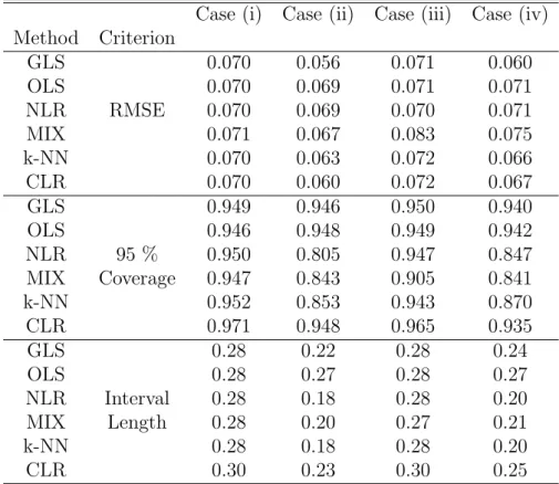
We repeat simulation exercise 1000 times for each DGP. The results are displayed in Table 1. Relative performance of the methods is similar whether RMSE,coverage, or interval length is used as an evaluation criterion. The results show that the conditional linear regression model proposed in this paper performs better than alternatives in Cases (ii) and (iv) in the presence of heteroscedasticity and performs comparably in other cases.

Table 1: Simulation results

Case (i) Case (ii) Case (iii) Case (iv) Method Criterion GLS 0.070 0.056 0.071 0.060 OLS 0.070 0.069 0.071 0.071 NLR RMSE 0.070 0.069 0.070 0.071 MIX 0.071 0.067 0.083 0.075 k-NN 0.070 0.063 0.072 0.066 CLR 0.070 0.060 0.072 0.067 GLS 0.949 0.946 0.950 0.940 OLS 0.946 0.948 0.949 0.942 NLR 95 % 0.950 0.805 0.947 0.847 MIX Coverage 0.947 0.843 0.905 0.841 k-NN 0.952 0.853 0.943 0.870 CLR 0.971 0.948 0.965 0.935 GLS 0.28 0.22 0.28 0.24 OLS 0.28 0.27 0.28 0.27 NLR Interval 0.28 0.18 0.28 0.20 MIX Length 0.28 0.20 0.27 0.21 k-NN 0.28 0.18 0.28 0.20 CLR 0.30 0.23 0.30 0.25

Notes: DGPs are in columns and methods of inference in rows. Entries are RMSE, Coverage of 95% Bayesian credibility region and interval length of the Bayesian credibility region. Bayesian inference in each method is implemented by a Gibbs sampler with 8000 draws and first 2000 discarded as burn-in for 1000 draws from each DGP.

In Cases (i) and (iii) the best performing models should be OLS and NLR since it is well know that OLS estimator achieves the semi-parametric efficiency under homoscedastic-ity. Note that model MIX performs worse in Cases (iii) and (iv) due to (conditional) asymmetries of the error distribution. In Case (iii) this is expected since the pseudo-true value of β is not the true β0 = 0 for the MIX model. As demonstrated in this simula-tion example estimasimula-tion of linear models with uncondisimula-tional error densities modeled as mixtures of normals or with flexible symmetric residual densities as proposed inPati and Dunson(2009) might be misguided if the regression coefficients are the object of interest. The reason being that the pseudo-true values ofβ might be different from the trueβ0, for

this paper outperforms other alternatives in the heteroscedastic cases and performs com-parably in the homoscedastic cases even when compared to the asymptotically efficient k-NN estimator.

5

Appendix

5.1

Proofs

Note that dKL is always non-negative, hence for any model Mm,n

0≤ Z log f0(y|x) p(y|x, θm,n,Mm,n) F0(dy, dx)≤ Z log max 1, f0(y|x) p(y|x, θm,n,Mm,n) F0(dy, dx).

Therefore, it would suffice to show that the last integral in the inequality converges to 0 as (m, n) increase. Dominated convergence theorem will be used for that. In the first part we will show pointwise convergence to 0 for any given (y, x) a.s. F. Then we will present conditions for the existence of an integrable upper bound on the integrand.

Pointwise Convergence

Let Am

j , j = 0,1, . . . , m, be a partition of Y, where Am1 , . . . , Amm are adjacent cubes

with side length hm and Am0 is the rest of set Y. Let Bnj, j = 0,1, . . . , N(n), be a

partition of X with N(n) =nd, where Bn₁, . . . , B_Nn_(n) are adjacent cubes with side length

λn and B0n is the rest of X. This partition has to satisfy two conditions. First, the

partition becomes finer as nincreases withλn →0. Second, the area covered by the finer

partition has to increase and eventually cover the whole support ofX, i.e. λd

nN(n)→ ∞.

Furthermore, let xn

i be the center of Bjn, j = 1, . . . , N(n) and xn0 ∈ B0n be such that

n ||xn 0 −x||2 > sn :∀x∈ SN(n) i=1 Bin o

a model Mm,n such that p(y|x,Mm,n) = N(n) X j=0 m X i=0 αnm_ji (x)φ y−h(x, θ);µji, σji2 (6) N(n) X j=0 m X i=0 αnm_ji (x)µji = 0 for allx∈ X.

We propose mixing probabilities such that

αnm_ji (x) = πjiαj(x) πji =F0(Ami |x n j) αj(x) = exp −cn(xnj 0_xn j −2xnj 0_x) PN(n) i=0 exp (−cn(xni 0_xn i −2xni 0_x)).

Under appropriate conditions for cn, we can show that some collection of αj(x)

ap-proximates 1Bn

j(x). All that is required is thatcn is such that cn→ ∞ and exp{−cnsn}/N(n)→0, where sn =λ2nd

i.e. sn is the squared diagonal of Bin. Such a sequence cn always exists, for

exam-ple all the necessary conditions would be satisfied for λn = N(n)−dn−1/2 = n−1/2 and

cn = s−n2. Following the proof of Proposition 4.1. in Norets (2010) define In(x, sn) =

j :||xn

j −x||2 < sn . Using the arguments of the proof of Proposition 4.1. we know that

for (n, m) large enough for any j ∈In_{(x, s} n)

X

j∈I1n(x,sn)

αj(x)≥1−exp{−cnsn}/N(n). (7)

Since h is Lipschitz continuous by Assumption 3, hence there exists L large enough such that |h(x, θ0)−h(xnj, θ0)| ≤ L||x−xnj||. Let δ

∗

m =δm+Ls

1/2

for any j ∈ I₁n(x, sn) and Ami ⊂ Cδ∗

m(y), where Cδ(y) is an interval centered at y with length δ, F0(Ami |x n j)≥λ(A m i ) inf z∈Cδ∗m(y),||t−x|| 2_≤s n f0(z|t). (8)

For each xn_j the parameters {µji} m i=0 must satisfy m X i=0 πjiµji = m X i=0 F0(Ami |x n j)µji = 0. (9)

Let θ = θ0, let cm_i be the center of the cube A_im if i 6= 0, then for i 6= 0 let µji =

cm

i +dnj −h(xnj, θ0) where djn∈[−hm/2, hm/2] and let µj0 be

µj0 = R Am 0 f0(y|x n j)(y−h(xnj, θ0))dy F0(Am0 |xnj)

ifF0(Am0 |xnj)>0 andµj0 = 0 otherwise. We show that there existsdnj such that equation

(9) is satisfied. Define functionG(dn

j|xnj) as G(dn_j|xn_j) = m X i=0 F0(Am_i |xn_j)µji = m X i=1 Z Am i f0(y|xnj)(c m i +d n j −h(x n j, θ0))dy+ Z Am 0 f0(y|xnj)(y−h(x n j, θ0))dy.

Clearly, the functionG(dn_j|x_jn) is linear in dn_j and therefore continuous in dn_j. Note that

G(hm/2|xnj) = m X i=1 Z Am i f0(y|xnj)(cmi +hm/2−h(xnj, θ0))dy+ Z Am 0 f0(y|xnj)(y−h(xnj, θ0))dy ≥ m X i=1 Z Am i f0(y|xnj)(y−h(x n j, θ0))dy+ Z Am 0 f0(y|xnj)(y−h(x n j, θ0))dy ≥ m X i=0 Z Am i f0(y|xn_j)(y−h(xn_j, θ0))dy = 0

since_EF0[y|x] =h(x, θ0) for allx∈ X and henceG(hm/2|x

n

j)≥0. By the same argument

it follows that 0 ≥G(−hm/2|xnj). As we have mentioned earlier G(·|xnj) is a continuous

function, therefore ∃ dn_j ∈[−hm/2, hm/2] such that G(dnj|xnj) = 0 and equivalently

equa-tion (9) is satisfied. For any j ∈ In_{(x, s} n) let y∗j = y−(h(x, θ0)−h(xnj, θ0)), then Cδm(y ∗ j) ⊂ Cδ∗ m(y) by definition of δm and δm∗. Let σji =σm if i>0 and σj0 =σ0 to be chosen later. Then for m large enough such that ∅ 6=i:Am

i ⊂Cδm(y∗) X i:Am i ⊂Cδm∗(y) λ(Am_i )φ y−h(x, θ0);µji, σm2 = X i:Am i ⊂Cδ_m∗(y) λ(Am_i )φ y−(h(x, θ0)−h(xnj, θ0));cmi +d n j, σ 2 m ≥ X i:Am i ⊂Cδm(y∗j) λ(Am_i )φ y∗_j;cm_i +dn_j, σ_m2 ≥1− 3hm (2π)1/2_σ m − 8σm (2π)1/2_δ m . (10)

with last inequality derived from Lemmas 1 and 2 in Norets and Pelenis (2012) (with a minor adjustment in the proofs due to uncentered positions of µji).

Then equation (6) and inequalities (7), (8) and (10) can be combined to show that for any given (x, y) there exist (m, n) large enough such that

p(y|x,Mm,n)> X j∈In 1(x,sn) X i:Am i ⊂Cδm∗(y) F0(Ami |x n j)αj(x)φ y−h(x, θ);µji, σm2 ≥ inf z∈C_δ∗ m(y),||t−x|| 2_≤s n f0(z|t) X j∈In 1(x,sn) αj(x) X i:Am i ⊂Cδ_m∗(y) λ(Am_i )φ y−h(x, θ);µji, σm2 ≥ inf z∈Cδ∗m(y),||t−x|| 2_≤s n f0(z|t) 1− 3hm (2π)1/2_σ m − 8σm (2π)1/2_δ m X j∈In 1(x,sn) αj(x) ≥ inf z∈Cδ∗_m(y),||t−x||2≤sn f0(z|t) 1− 3hm (2π)1/2_σ m − 8σm (2π)1/2_δ m 1− exp{−cnsn} N(n)

Let {δm, σm, hm, cn, sn} satisfy the following:

δm →0, σm/δm→0, hm/σm →0, cn→ ∞, sn →0, exp{−cnsn}/N(n)→0.

Hence for any given (x, y) and a given >0 there exist (M1, N1) large enough such that

∀m > M1, n > N1 p(y|x,Mm,n)> inf z∈Cδ∗m(y),||t−x|| 2_≤s n f0(z|t)·(1−).

By Assumption 1 f0(y|x) is continuous in (y, x) and if f0(y|x) > 0, then there exist

(M2, N2) large enough such that ∀m > M2, n > N2 f0(y|x)

infz∈Cδ∗m(y),||t−x||

2_≤s

nf0(z|t)

≤1 +

since sn →0 andδm∗ →0. Then for any (m, n)≥ {max{M1, M2},max{N1, N2}}

1≤ f0(y|x) p(y|x,Mm,n) ≤ f0(y|x) infz∈Cδm∗(y),||t−x|| 2_≤s nf0(z|t)(1−) ≤ 1 + 1−.

Henceforth, log max{1, f0(y|x)/p(y|x,Mm,n)} →0 a.s. F0as long asf0(y|x) is continuous

in (y, x) a.s. F0. This result establishes pointwise convergence.

Integrable upper bound

Now we will establish an integrable upper bound for the application of the DCT. We know from equation (7) that for any x∈ X there existsn large enough such thatαj(x)>1/2

for j ∈ In_{(x, s}

n). Similarly from equation (10) that for any (y, x) the bound for the

Riemann sum is bounded below by 1/2 for m large enough. These facts will be used in deriving an integrable upper bound.

Before we proceed one additional change to the model Mm,n has to be made. Note

j. We define a new model M∗

m,n by introducing πj00 = 0.5F0(Am0 |Xjn) and µj00 = 0 and πj01= 0.5F0(Am0 |Xjn) and µj01 = 2µj0. Then for j ∈In(x, sn) and n, m large enough

p(y|x,M∗_m,n) = N(n) X j=1 αj(x) M X m=1 F0(Ami |x n j)φ y−h(x, θ);µji, σm2 + 0.5F0(Am0 |X n j)φ y−h(x, θ); 2µj00, σ02 + 0.5F0(Am0 |X n j)φ y−h(x, θ); 0, σ 2 0 > αj(x) M X m=1 F0(Ami |x n j)φ y−h(x, θ);µji, σ2m + 0.5F0(Am0 |X n j)φ y−h(x, θ); 0, σ 2 0 ! >0.5[1−1Am 0 (y)] inf z∈Cδ_m∗(y),||t−x||2≤δ f0(z|t) X i:Am i ⊂Cδ∗m(y) λ(Am_i )φ y−h(x, θ);µji, σm2 + 0.25·1Am 0 (y)F0(A m 0 |X n j)φ y−h(x, θ); 0, σ 2 0 >0.25[1−1Am 0 (y)] inf z∈Cδ∗m(y),||t−x|| 2_≤δf0(z|t) + 0.25·1Am 0 (y)_z∈C inf δ(y),||t−x||2≤δ f0(z|t)·λ(Cδ(y))φ y−h(x, θ); 0, σ20 >0.25[1−1Am 0 (y)]_z∈C inf δ(y),||t−x||2≤δ f0(z|t) + 0.25·1Am 0 (y)_z∈C inf δ(y),||t−x||2≤δ f0(z|t)·δ·φ y−h(x, θ); 0, σ02 >0.25 inf z∈Cδ(y),||t−x||2≤δ f0(z|t)·δ·φ y−h(x, θ); 0, σ20

form, nlarge enough such thatδ∗_m< δ,sn< δandσ02chosen such thatδφ(y−h(x, θ); 0, σ20)<

1. Then log max 1, f0(y|x) p(y|x, θ,M∗ m,n) ≤log max 1, f0(y|x) 0.25δφ(y−h(x, θ); 0, σ2 0) infz∈Cδ(y),||t−x||2≤δf0(z|t) = log 1 0.25δφ(y−h(x, θ); 0, σ2 0) · f0(y|x) inf_z∈Cδ(y),||t−x||2≤δf0(z|t) =−log0.25δφ y−h(x, θ); 0, σ2₀ + log f0(y|x) infz∈Cδ(y),||t−x||2≤δf0(z|t)

is integrable by Assumption 4.

In summary, applying DCT we get that dKL(f0(·|·), p(·|·, θ,Mm,n))→0.

Finite model with mixtures of two normal distributions

The final component of the proof is to show that the model Mm,n can be rewritten as

a finite regressor dependent mixture of f2 rather than just Gaussian densities. We start

with a finite model as defined in equation (6)

p(y|x,Mm,n) = n X j=0 αj(x) m X i=0 πjiφ y−h(x, θ);µji, σji2 .

Given any j by Lemma 1 below there exists

pji, πji∗, µ ∗ ji, σ2 ∗ ji m i=0 m X i=0 πjiφ y−h(x, θ);µji, σ2ji = m X i=0 pji 2 X l=1

π_jil∗ φ y−h(x, θ);µ∗_jil, σ_jil2∗

such that Pm i=0pji = 1, P2 l=1π ∗ jil = 1 and P2 l=1π ∗ jilµ ∗

jil = 0 for all i. Note that predictor

dependent weights can be expressed as

αj(x) = exp −cn(xnj 0_xn j −2xnj 0_x) Pn i=0exp (−cn(x n i 0_xn i −2xni 0_x)) = exp (φj,0+φj,−0x) Pn i=0exp (φi,0+φi,−0x)

constructed using Lemma 1 for each j. Then p(y|x,Mm,n) = n X j=0 αj(x) m X i=0 πjiφ y−h(x, θ);µji, σji2 = n X j=0 exp (φj,0+φj,−0x) Pn k=0exp (φk,0+φk,−0x) m X i=0 πji 2 X l=1

π∗_jilφ y−h(x, θ);µ∗_jil, σ2_jil∗

= n X j=0 m X i=0

exp φ∗_ji,0+φ∗_ji,−0x

Pn k=0exp φ ∗ k,0+φ ∗ k,−0x 2 X l=1

π∗_jilφ y−h(x, θ);µ∗_jil, σ2_jil∗

= m×n X j=0 exp φ∗_j,0+φ∗_j,−0x Pn×m k=0 exp φ ∗ k,0+φ ∗ k,−0x 2 X l=1 π_jl∗φ y−h(x, θ);µ∗_jl, σ2_jl∗.

This shows that modelMm,n can be represented using a finite predictor-dependent

mix-ture of 2-component mixmix-ture models with mean zero.

Lemma 1. Let θn ={πi, µi, σ2i} n i=1 be such that p(y|θn) = n X i=1 πiφ(y;µi, σi2) such that Pn i=1πi = 1 and Pn

i=1πiµi = 0. Then there exists a set of parameters θ∗n =

{p∗_i, π∗_i1, µ∗_i1, σ2_i1∗, π_i∗₂, µ∗_i2, σ_i2₂∗}n_i=1 such that p(y|θn) =p(y|θn∗) = n−1 X i=1 p∗_i 2 X l=1 π_il∗φ(y;µ∗_il, σ2_il∗) such that Pn−1 i=1 p ∗ i = 1, P2 l=1π ∗ il = 1 and P2 l=1π ∗ ilµ∗il = 0 for each i. Proof. (Lemma1)

Find i= arg mini∈{1,...,n}{|πiµi|}. Let i=n without loss of generality. If µi = 0 then let

p∗₁ =πi andπ11∗ =π ∗ 12 = 1/2,µ ∗ 11 =µ ∗ 12=µi andσ122∗ =σ2 ∗

11 =σ2i. If µi 6= 0, then pick any

j 6=i such that sign(µi)=6 sign(µj). Then let π∗11= (p

∗ 1) −1_π i and π∗12= (p ∗ 1) −1_π i|µi|/|µj|

and σ₁₂2∗ =σ2_j. ThenP2 l=1π ∗ il = 1 and P2 l=1π ∗ ilµ ∗ il = 0 for i= 1.

Let ˜πk = πk for all k = 1, . . . , j−1, j + 1, . . . , n−1 and let ˜πj = πj −πn|µn|/|µj|.

Then n X i=1 πiφ(y;µi, σi2) = n−1 X i=1 ˜ πiφ(y;µi, σi2) +p ∗ 1 2 X l=1 π₁∗_lφ(y;µ∗_1l, σ2_1l∗). By induction n X i=1 πiφ(y;µi, σi2) = n−1 X i=1 p∗_i 2 X l=1 π₁∗_lφ(y;µ∗_1l, σ2_1l∗) where P2 l=1π ∗ il = 1 and P2 l=1π ∗

ilµ∗il = 0 for each i. Note that

Pn−1

i=1 p

∗

i = 1 since integral

of the LHS w.r.t y is 1 and integral of RHS w.r.t y is 1 iff Pn

i=1p

∗

i = 1.

Proof. (Theorem 2)

We want to show that f0 ∈ KL(Π), that is Π({(θ, η) :dKL(f0(·,·), p(·|·, θ, η)< }) >0.

Let >0 be given. By Thoerem1 there exists a finite numberk and a set of parameters (ηk, θ) such that dKL(f0(·|·), p(·|·, θ, ηk))< /3, where ηk =

πj, µj, σj1, σj2, γj0 k

j=1. Note

that the mixing weights that depend on {ρj, γj0}kj=1 can be rewritten as

αj(x) = exp ρj+γj0x Pk l=1exp (ρl,0+γl0xi) = exp ρj+γ 0 jγj/2−γj0γj/2 +γj0x−x 0_x Pk l=1exp (ρl+γl0γl/2−γl0γl/2 +γl0x−x0x) = exp (ρj +γ 0 jγj/2)−0.5||x−γj||2 Pk l=1exp ((ρl+γ 0 lγl/2)−0.5||x−γl||2) ≡ αjexp (−ϕ||x−Γj|| 2₎ Pk l=1αlexp (−ϕ||x−Γl||2) = αjKϕ(x,Γj) Pk l=1αlKϕ(x,Γl)

with a set of parameters {ϕ, αj,Γj}kj=1. In this particular construction ϕ= 0.5, however

Let fF SM R(·|·, θ, ηk) be constructed as fF SM R(y|x, θk) = k X j=1 pj(x)f2(y−h(x, θ);πj, µj, σj1, σj2) pj(x) = αjKϕ(x,Γj) Pk l=1αlKϕ(x,Γl)

and we know that dKL(f0(·,·), fSM R(·|·, θ, ηk)) < /3 for some particular parameters

(θ, ηk). Now, we will show that there exists a truncated at some largeK infinite smoothly

mixing regression fT SM R such that

Z log fSM R(y|x, θ, ηk) fT SM R(y|x, θ, ηK) dF0(y, x)< 3 where fT SM R(yi|xi, θ, ηK) = K X j=1 pj(xi)f2(yi−h(xi, θ);πj, µj, σj1, σj2) pj(x) =VjKϕ(x,Γj) Y l<j (1−VlKϕ(x,Γl)).

Let’s construct an infinite smoothly mixing regression with parameters (θ∗, η∗) based on the parameters (θ, ηk) of fSM R. Let θ∗ =θ, and η∗ ≡

π_j∗, µ∗_j, σ_j∗₁, σ_j∗₂, V_j∗,Γ∗_j0 k j=1 be defined as (π∗_h, µ∗_h, σ_h∗₁, σ_h∗₂) = (π∗, µ∗₁, σ₁∗, σ∗₂)(h modk)= (πj, µj2, σj1, σj2) Kϕ(x,Γ∗h) =Kϕ(x,Γ∗(h modk)) =Kϕ(x,Γj) V_h∗ =V₍∗_{h modk)} =αj ·δ

where j = (h modk) and for some smallδ with max{αj}

−1

> δ >0 and any ϕ >0. Given these parameter values of η∗ the conditional density induced by the infinite

smoothly mixing representation is fISM R(y|x, θ∗, η∗) = k X j=1 δαjKϕ(x,Γj)f2(y−h(x, θ);πj, µj, σj1, σj2) Y 0<l<j (1−δαlKϕ(x, xl)) + 2·k X j=k+1 δαjKϕ(x, xj)f2(y−h(x, θ);πj, µj, σj1, σj2) Y k<l<j (1−δαlKϕ(x, xl)) · Y 0<i≤k (1−δαiKϕ(x, xl)) + 3·k X j=2·k+1 δαjKϕ(x, xj)f2(y−h(x, θ);πj, µj, σj1, σj2) Y 2·k<l<j (1−δαlKϕ(x, xl)) · Y 0<i≤2·k (1−δαiKϕ(x, xl)) +. . . and it combines to fISM R(y|x, θ∗, η∗) = Pk j=1δαjKϕ(x, xj)f2(y−h(x, θ);πj, µj, σj1, σj2)· Q l<j(1−δαlKϕ(x, xl)) Pk j=1δαjKϕ(x, xj) Q l<j(1−δαlKϕ(x, xl)) .

It is almost immediate that fIM SR(y|x) induced by infinite representation approaches

fSM R(y|x, θ, ηk) for all values of (y, x) as δ → 0. To make this statement precise note

that fSM R(y|x, θ, ηk) fIM SR(y|x, θ∗, η∗) = Pk j=1αjKϕ(x, xj)f2(y−h(x, θ);πj, µj, σj1, σj2) Pk j=1αjKϕ(x, xj)f2(y−h(x, θ);πj, µj, σj1, σj2) Q l<j(1−δαlKϕ(x, xl)) · Pk j=1αjKϕ(x, xj) Q l<j(1−δαlKϕ(x, xl)) Pk j=1αjKϕ(x, xj) < Pk j=1αjKϕ(x, xj)f2(y−h(x, θ);πj, µj, σj1, σj2) Pk j=1αjKϕ(x, xl)f2(y−h(x, θ);πj, µj, σj1, σj2)·(1−δmaxαl)k ·1 = 1 (1−δmaxαl)k .

Then if we pick δ <(1−exp(−/(6k)))/max{αj} it immediately implies that

log(fSM R(y|x, θ, ηk)/fISM R(y|x, θ, η∗)) < /6 for all (y, x). Now we want to show that

there exists fT SM R such that log(fISM R(y|x, θ, η∗)/fT SM R(y|x, θ, ηK)) < /6. Let the

truncated SMR be cut off at a point K = k ∗M for some M large enough. Then by construction of η∗ for any (y, x) the following is true

fISM R(y|x, θ, η∗) 1− Y 1≤l<k∗M (1−δαlKϕ(x,Γl) ! =fT SM R(y|x, θ, ηK) fISM R(y|x, θ, η∗) fT SM R(y|x, θ, ηK) = 1− Y 1≤l<k∗M (1−δαlKϕ(x,Γl) !−1

The objective is to show thatM large enough exists such that

−log 1− Y

1≤l<k∗M

(1−δαlKϕ(x,Γl)

!

< /6.

This is achieved by considering let i∗ = arg maxj=1,···,k{αj}. Since X is bounded we can

find K = maxx∈XKϕ(x,Γi∗)>0. Then

−log 1− Y 1≤l<k∗M (1−δαlKϕ(x,Γl) ! <−log 1− Y 1≤l<M (1−δαi∗K) ! =−log 1−(1−δαi∗K)M.

Then for M > log(1−e−/6) log(1−δαi∗K)

this inequality is true

−log 1−(1−δαi∗K)M< /6.

Hence, forK > k∗M we have foundηK_{such that log(f}

/6 for all (y, x) and it follows that Z log fSM R(y|x, θ, ηk) fT SM R(y|x, θ, ηK) dF0(y, x)< 3.

Next we will show that there exists an open neighborhood Υ of ηK such that for any

η0 ∈Υ Z log fT SM R(y|x, θ, ηK) fT SM R(y|x, θ, η0) dF0(y, x)< 3.

To show this we will show that this integral is (sequentially) continuous in η0 at ηK. Let

ηl be a sequence of parameter values converging to ηK asl → ∞. Then for every (y, x),

we have that log(fT SM R(y|x, θ, ηK)/fT SM R(y|x, θ, ηl)) →1. To show that the integral is

continuous we will use the dominated convergence theorem. We need to show that there exist integrable with respect to F0 lower and upper bounds for −log(fT SM R(y|x, θ, ηl)).

Since, fT SM R(yi|xi, θ, ηl) = K X j=1 pj(xi)f2(yi−h(xi, θ);πj, µj, σj1, σj2) As ηl _→η

K, therefore for l large enough and for some finiteµ > µ, σ > σ and π > π we

will find that πl

j ∈(π, π),µlj ∈(µ, µ), −µlj πl j 1−πl j ∈(µ, µ) and σl j1, σjl2 ∈(σ, σ). Then φ(0; 0, σ)≥fT SM R(yi|xi, θ, ηl) ≥ 1(−∞,µ)exp −(y₂−_σµ2)2 + 1(µ,µ)exp −(µ₂−_σµ2)2 + 1(µ,∞)exp −(y₂−_σµ2)2 √ 2πσ2 .

The logarithm of the upper bound is constant and finite, hence integrable. The logarithm of the lower bound is integrable by the Assumption2of the Theorem1as the conditional second moments of y are finite under F0. Hence the integral is continuous and an open

neighborhood Υ of ηK exists.

Finally, given any η0 ∈Υ, let η∞= (η0, ηK+1:∞) withηK+1:∞ unrestricted. Then

log fT SM R(y|x, θ, η

0₎

fISM R(y|x, θ, η∞)

<0

for any (y, x) by definition.

In conclusion, then there exists ηK and an open neighborhood Υ of ηK such that for

any η0 ∈Υ and anyη∞= (η0,·)

Z log f0(y|x) fISM R(y|x, θ, η∞) dF0(y, x) = Z log f0(y|x) fSM R(y|x, θ, ηk) dF0(y, x) + Z log fSM R(y|x, θ, ηk) fT SM R(y|x, θ, ηK) dF0(y, x) + Z log fT SM R(y|x, θ, ηK) fT SM R(y|x, θ, η0) dF0(y, x) + Z log fT SM R(y|x, θ, η 0₎ fISM R(y|x, θ, η∞) dF0(y, x) < 3 + 3 + 3 + 0< .

Hence, if ηk is in the support of the prior and the priors assign a positive mass for some

neighborhood of anyηk, then Π(Υ)>0 andf0 is in the KL support of Π.

Proof. (Theorem 3)

First, we would like to construct an unbiased test for the hypothesis:

H0 : (f, θ) = (f0, θ0) against H1 : (f, θ)∈ V × {θ :||θ−θ0|| ≥ρ}

where V = supp(Πf|x). To do so we will consider a finite set of alternative hypothesis such that their union would be a superset of H1. Therefore, consider for some small

∆>0 a group of hypothesis for each γ and j = 1, . . . , d

For anyj consider onlyxobservations such thatxjγj > ξ wherexj is thej−th coordinate

of x and x ∈ Qγ, then by construction x0θ−x0θ0 > ξ∆. Let Qγ,j =Qγ\{X : |xj| < ξ},

then by the assumption of the theorem F0(Qγ,j) =ζ >0. Then we will use Chebyshev’s

inequality to construct strictly unbiased test for H0 against H1. By assumptions 1 and

2 of Theorem 1 there exists M such that M > supx∈XEF0[(y−x

0_θ

0)2|x]. For any n let Kn,j = Pn i=11{xi ∈ Qγ,j}. Then let Tn,j = Kn,j−1 Pn i=11{xi ∈ Qγ,j}(yi −xiθ0). Then by Chebyshev’s inequality Pf0(|Tn,j| ≥ ε) ≤ M2

Kn,jε2 and since ζ > 0 it is immediate that

Pf0(|Tn,j| ≥ ε) → 0 as n → ∞. Now we just need to show that inf(f,θ)∈H1Pf,θ(|Tn,j| ≥

ε)→1 as n → ∞. Then note that for any θ∈H1, we have that x0θ−x0θ0 > ξ∆. So let ε=ξ∆/3 and consider a statistic ˜Tn,j =Kn,j−1

Pn

i=11{xi ∈Qγ,j}(yi−xiθ). Then

Pf,θ(|Tn,j| ≥ε)≥Pf,θ(|T˜n,j| ≤ε)≥1−

L2 Kn,jε2

whereL > supx∈X,f∈W,θ∈ΘEf,θ[(y−x0θ)2|x] for some L by conditions on the prior support.

Since Kn,j → ∞ as n → ∞, therefore Pf,θ(|Tn,j| ≥ ε) → 1. These facts can be used to

construct an uniformally consistent sequence of tests

φn(Xn, Yn) = 1{|Tn,j| ≥ξ∆/3}

and by Proposition 4.4.1 byGhosh and Ramamoorthi (2003) this implies the existence of exponentially consistent tests. Note that by choosing ∆ >0 sufficiently small the union of these sets of alternative hypothesis will contain the set{(f, θ)∈ V ×{θ :||θ−θ0|| ≥ρ}}

which is the original alternative hypothesis.

Given a weak neighborhood of Uδ(f0,|x) of conditional error density, let’s construct

exponentially consistent tests for this hypothesis:

for some smallυ >0. Uδ(f0,|x) is defined via some bounded uniformly continuous function

g, then let ∆2 be such that if |1 −2| < ∆2, then |g(1, x)−g(2, x)| < δ/2. Then for f|x ∈ Uδ(f0,|x)cand anyθsuch that|θ−θ0|< υ, whereυis such that|x0(θ−θ0)|<∆2asX

is bounded, definefy|x,θ =f|x(+h(x, θ), x). Then fy|x,θ ∈ Uδ/2(f0,y|x)c whereUδ/2(f0,y|x)

is a weak neighborhood of conditional densitiesf0(y|x). Exponentially consistent tests for

such weak neighborhoods always exist, while we could not have constructed exponentially consistent tests based on unobservable .

By choosing ∆ and υ small enough the union of the sets of alternative hypothesis would contain{(f|x, θ)∈ Uδ(f0,|x)c× {θ :||θ−θ0|| ≥ρ}}. Then exponentially consistent

tests for H0 : (f, θ) = (f0, θ0) against H1 : (f, θ)∈(Uδ(f0,|x)× {θ:||θ−θ0||< ρ})c exist,

and since f0 ∈ KL(Π) by Theorem 2, then a straightforward application of Schwartz

(1965) posterior consistency theorem yields the result that Π(Wc_|Y

n, Xn) → 0 a.s. PF∞0

for any given ρ >0.

Proof. (Corollary1)

First, we would like to construct an unbiased test for the hypothesis:

H0 : (f, θ) = (f0, θ0) against H1 : (f, θ)∈ V × {θ :||θ−θ0|| ≥ρ}

where V = supp(Πf|x).

By the assumption 2 of Theorem 1 there exists M such that M > supx∈XEF0[(y−

h(x, θ0))2|x]. LetTn=n−1

Pn

i=1yi−h(xi, θ0). Then by Chebyshev’s inequalityPf0(|Tn| ≥

ε) ≤ M2

nε2 and it is immediate that Pf0(|Tn| ≥ ε) → 0 as n → ∞. Now we just need to

show that inf(f,θ)∈H1Pf,θ(|Tn| ≥ ε) → 1 as n → ∞. Then note that for any θ ∈ H1,

˜ Tn =n−1 Pn i=1yi−h(xi, θ). Then Pf,θ(|Tn| ≥ε)≥Pf,θ(|T˜n| ≤ε)≥1− L2 nε2

where L > supx∈X,f∈W,θ∈ΘEf,θ[(y−h(x, θ))2|x] for some L by conditions on the prior

support. Since n → ∞, therefore Pf,θ(|Tn| ≥ ε) → 1. These facts can be used to

construct an uniformly consistent sequence of tests

φn(Xn, Yn) = 1{|Tn| ≥ξρ/3}

By Proposition 4.4.1 by Ghosh and Ramamoorthi (2003) this implies the existence of exponentially consistent tests. The rest of the proof is identical to the Theorem 3.

5.2

Posterior Computation

The finite model with k states is defined as

p(yi|xi, β, ηk) = k X j=1 αj(xi)f2 yi−x 0 iβ;πj, µj, h −1/2 j1 , h −1/2 j2 αj(xi) = exp ρj +γj0xi Pk l=1exp (ρl+γ 0 lxi) .

We propose Gibbs sampler for the estimation procedure. We introduce latent state vari-ables si = (si1, si2) with si1 ∈ {1, . . . , k} and si2 ∈ {1,2}. Then p(yi|si, xi, β, ηk) =

φ(·, xi0β +µsi, h −1 si ), with µj1 = µj and µj2 = − πj 1−πjµj and P(si = (j, l)|xi, β, ηk) = αj(xi)πjl.

Gibbs sampling techniques byGeweke and Amisano(2011) are employed to implement the zero mean conditions in Gibbs sampler. Letsi = (j, l), then define di as 2k×1 vector

with value 1 on (2(j−1) +l)’th row and 0 elsewhere. Letπj be the j’th row ofπ, then let

2×1 vector Cj be the orthonormal compliment of πj. Define scalar ˜µj =Cj0(µj1, µj2)0.

Construct 2k×k matrix C = Blockdiag[C1, . . . , Ck] and k×1 vector ˜µ = (˜µ1, . . . ,µ˜k)0.

Then the distribution of observable yi is

(yi|xi, si, β, ηk)∼N(xi0β+ ˜µ0C0di, h−si1).

Letζ = (β0,µ˜0)0 and Wi = (Xi0, d0iC). Finally,the distribution of observable yi is

(yi|xi, si, β, ηk)∼N(Wiζ, h−si1)

and the prior for ζ is induced by priors on ˜µ and β. The following priors are used: Gaussian priors for β, ρ, γ,µ˜, a Gamma prior for h2 _{and a Dirichlet prior for π. The full}

posterior is proportional to the joint distribution of observables and unobservables: p(YN, SN, β, ηk|XN)∝ N Y i=1 |hsi| 1/2_exp −0.5(yi−Wiζ)2hsi αsi1(xi)πsi · |H_ζ|1/2_exp −0.5(ζ−ζ)0H_ζ(ζ−ζ) · k Y j=1 2 Y l=1 π_jlπ−1 · k Y j=1 2 Y l=1 |hjl|(ν−2)/2exp −0.5s2hjl · k Y j=1 |H_γ|1/2_exp −0.5(γj −γ)0Hγ(γj−γ) · k Y j=1 |H_ρ|1/2_exp −0.5(ρj −ρ)0Hρ(ρj −ρ) where ζ = [β0,00]0 , H_µ=h_µ·Ik, H_ζ =    H_β 0 0 H_µ   .

Then Gibbs sampler consists of:

1. Conditional posterior distribution of ζ:

p(ζ|. . .)∼Nζ, H−_ζ1 Hζ =Hζ+ N X i=1 W_i0hsiWi ζ =H−_ζ1 H_ζζ+ N X i=1 W_i0hsiyi ! .

2. Conditional posterior distribution of hjl: hjl ∼Ga   ν+Njl 2 ,   1 2s 2 + 1 2 X i|si=(j,l) (yi−Wiζ)(yi −Wiζ)0   −1  where Njl=PN_i=11{si=(j,l)}.

3. Conditional posterior distribution of π:

Posterior distribution ofπ is non-standard and non-conjugate since C is a function of π and we must account for that in our posterior simulator. Firstly, we will follow Geweke and Amisano (2011) in producing a unique representation of Cj for

j = 1, . . . , k. Note thatπjCj = 0, then construct uniqueCj by first constructingCj∗

as follows: C_j∗ = (πj1,−πj21/πj2)0. Then construct uniqueCj by normalizing column

of C_j∗ to Euclidean length of 1. Since Cj is a function of π, we will use Metropolis

within Gibbs step for each row j of π. Use Dirichlet distribution as a proposal for row πj p(πj|. . .)∝π (π+Nj1) j1 π (π+Nj2) j2 .

Construct new ∗_i =yi−Wi∗ζ. Then Metropolis acceptance ratio for the new draw

of πj is exp−0.5P i|si1=j ∗0 i hsi ∗ i exp−0.5P i|si1=j 0 ihsii where i =yi−Wiζ.

4. Conditional posterior distribution of (ρ, γ):

5. Conditional posterior distribution of si:

Gibbs sampler block forsi has a simple multinomial distribution with

p(si = (j, l)|. . .)∝αj(xi)πjl|hjl|0.5exp{−0.5(yi−µjl−x0iβ)

0

hjl(yi−µjl−x0iβ)}.

References

Amewou-Atisso, M., Ghosal, S., Ghosh, J. K., and Ramamoorthi, R. V. Posterior con-sistency for semi-parametric regression problems. Bernoulli, 9(2):291–312, 2003.

Chung, Y. and Dunson, D. The local dirichlet process.Annals of the Institute of Statistical Mathematics, 63(1):59–80, 2011.

Chung, Y. and Dunson, D. B. Nonparametric bayes conditional distribution modeling with variable selection.Journal of the American Statistical Association, 104(488):1646– 1660, 2009.

Conley, T. G., Hansen, C. B., McCulloch, R. E., and Rossi, P. E. A semi-parametric bayesian approach to the instrumental variable problem. Journal of Econometrics, 144(1):276 – 305, 2008.

De Iorio, M., Mller, P., Rosner, G. L., and MacEachern, S. N. An anova model for depen-dent random measures. Journal of the American Statistical Association, 99(465):205– 215, 2004.

Dunson, D. B. and Park, J.-H. Kernel stick-breaking processes. Biometrika, 95(2):307– 323, 2008.

Geweke, J. and Amisano, G. Hierarchical markov normal mixture models with applica-tions to financial asset returns. Journal of Applied Econometrics, 26(1):1–29, 2011.

Geweke, J. and Keane, M. Smoothly mixing regressions. Journal of Econometrics, 138(1):252–290, 2007.

Ghosh, J. K. and Ramamoorthi, R. V. Bayesian Nonparametrics. Springer, New York, 2003.

Griffin, J. E. and Steel, M. F. J. Order-based dependent dirichlet processes. Journal of the American Statistical Association, 101(473):179–194, 2006.

Hirano, K. Semiparametric bayesian inference in autoregressive panel data models.

Econometrica, 70(2):781–799, 2002. ISSN 00129682.

Jacobs, R. A., Jordan, M. I., Nowlan, S. J., and Hinton, G. E. Adaptive mixtures of local experts. Neural Computation, 3(1):79–87, 1991.

Kalli, M., Griffin, J. E., and Walker, S. G. Slice sampling mixture models. Statistics and Computing, 21(1):93–105, 2011.

Kleijn, B. J. K. and Bickel, P. J. The semiparametric bernstein-von mises theorem.

Working paper, 2010.

Kottas, A. and Gelfand, A. E. Bayesian semiparametric median regression modeling.

Journal of the American Statistical Association, 96(456):1458–1468, 2001.

Kottas, A. and Krnjajic, M. Bayesian nonparametric modeling in quantile regression.

Scandinavian Journal of Statistics, 36(2):297–319, 2009.

Lancaster, T. A note on bootstraps and robustness. Working paper, 2003.

Leslie, D. S., Kohn, R., and Nott, D. J. A general approach to heteroscedastic linear regression. Statistics and Computing, 17(2):131–146, 2007.

MacEachern, S. N. Dependent nonparametric processes. ASA Proceedings of the Section on Bayesian Statistical Science, 1999.

Muller, P., Erkanli, A., and West, M. Bayesian curve fitting using multivariate normal mixtures. Biometrika, 83(1):67–79, 1996.

M¨uller, U. K. Risk of bayesian inference in misspecified models and the sandwich covari-ance matrix. Working paper, 2010.

Norets, A. Approximation of conditional densities by smooth mixtures of regresssions.

Annals of Statistics, 38(3):1733–1766, 2010.

Norets, A. and Pelenis, J. Posterior consistency in conditional density estimation by covariate dependent mixtures. Working paper, 2011.

Norets, A. and Pelenis, J. Bayesian modeling of joint and conditional distributions.

Journal of Econometrics, forthcoming, 2012.

Papaspiliopoulos, O. and Roberts, G. O. Retrospective markov chain monte carlo meth-ods for dirichlet process hierarchical models. Biometrika, 95(1):169–186, 2008.

Pati, D., Dunson, D., and Tokdar, S. Posterior consistency in conditional distribution estimation. Working paper, 2011.

Pati, D. and Dunson, D. B. Bayesian nonparametric regression with varying residual density. Working paper, 2009.

Robinson, P. M. Asymptotically efficient estimation in the presence of heteroskedasticity of unknown form. Econometrica, 55(4):875–891, 1987.

Schwartz, L. On bayes procedures. Z. Wahrsch. Verw. Gebiete, 4:10–26, 1965.

Shen, X. Asymptotic normality of semiparametric and nonparametric posterior distribu-tions. Journal of the American Statistical Association, 97(457):222–235, 2002.

van der Vaart, A. W. Asymptotic Statistics. Cambridge University Press, 1998.

Walker, S. G. Sampling the dirichlet mixture model with slices. Communications in Statistics - Simulation and Computation, 36(1):45–54, 2007.

White, H. Maximum likelihood estimation of misspecified models.Econometrica, 50(1):1– 25, 1982.

Wu, Y. and Ghosal, S. Posterior consistency for some semi-parametric problems. Sankhya : The Indian Journal of Statistics, 70(3):0–46, 2008.

Author: Justinas Pelenis

Title: Bayesian Semiparametric Regression Reihe Ökonomie / Economics Series 285 Editor: Robert M. Kunst (Econometrics)

Associate Editors: Walter Fisher (Macroeconomics), Klaus Ritzberger (Microeconomics) ISSN: 1605-7996

© 2012 by the Department of Economics and Finance, Institute for Advanced Studies (IHS),