Developing Leading and Lagging Indicators to Enhance Equipment Reliability in a Lean System

University of Tennessee, Knoxville

Trace: Tennessee Research and Creative

Exchange

Masters Theses Graduate School

12-2017

Developing Leading and Lagging Indicators to

Enhance Equipment Reliability in a Lean System

Dhanush Agara Mallesh

University of Tennessee, Knoxville, [email protected]

This Thesis is brought to you for free and open access by the Graduate School at Trace: Tennessee Research and Creative Exchange. It has been accepted for inclusion in Masters Theses by an authorized administrator of Trace: Tennessee Research and Creative Exchange. For more information, please [email protected].

Recommended Citation

Agara Mallesh, Dhanush, "Developing Leading and Lagging Indicators to Enhance Equipment Reliability in a Lean System. " Master's Thesis, University of Tennessee, 2017.

To the Graduate Council:

I am submitting herewith a thesis written by Dhanush Agara Mallesh entitled "Developing Leading and Lagging Indicators to Enhance Equipment Reliability in a Lean System." I have examined the final electronic copy of this thesis for form and content and recommend that it be accepted in partial fulfillment of the requirements for the degree of Master of Science, with a major in Industrial Engineering.

Rapinder Sawhney, Major Professor We have read this thesis and recommend its acceptance:

Xueping Li, Russell Zaretzki

Accepted for the Council: Carolyn R. Hodges Vice Provost and Dean of the Graduate School (Original signatures are on file with official student records.)

Developing Leading and Lagging

Indicators to Enhance Equipment

Reliability in a Lean System

A Thesis Presented for the

Master of Science

Degree

The University of Tennessee, Knoxville

Dhanush Agara Mallesh

December 2017

©by Dhanush Agara Mallesh, 2017 All Rights Reserved.

For my parents, Appa and Amma, and Akka and Arjun, and, my godson Leo.

Acknowledgements

I am extremely thankful and indebted to my advisor Dr. Rupy Sawhney for guidance through the course work and progress of this master’s thesis. His constant support and encouragement will always be remembered. In addition to helping me academically, he showered me with many fatherly advice, and also put me in situations where I gained opportunities to improve professionally.

My appreciation also goes to Dr. Xueping Li and Dr. Russell Zaretzki for being a part of my thesis committee, and also being a constant source of motivation throughout the course of the program. The staff and faculty of the Department of Industrial and System Engineering at the University of Tennessee provided a friendly environment. In particular, my gratitude goes to Carla Arbogast for her words of encouragement and guidance during job applications, and, Enrique Macias De Anda, Dr. Ninad Pradhan, Dr. Kaveri Thakur and Vahid Ganji for their endless hours of help and dedication to all the students in Department of Industrial Engineering, and particularly to me. I am extremely thankful to Meridium, Inc. for their co-operation and willingness to work on this research. Special regards to Sarah Lukens who I could bounce ideas off and played a vital role in the completion of this research.

My colleagues and friends Bharadwaj, Guru, Dinesh, Samantha, Kapil, Abhishek, Mohit, Mozzie, Mostafa, Justin, Anju, Girish, Wolday, Julia, Bill, and other in CASRE group also deserve special mention.

Selfless affection and dedication offered by my parents Mallesh and Shantha cannot be expressed in words. My utmost indebtedness to Kavya and Arjun who helped throughout my graduate school starting from admission until I found a job.

“Do. Or do not. There is no try.”

—Jedi Master Yoda, Star Wars

“If you can find a path with no obstacles, it probably doesn’t lead anywhere”

— Frank A. Clark

Abstract

With increasing complexity in equipment, the failure rates are becoming a critical metric due to the unplanned maintenance in a production environment. Unplanned maintenance in manufacturing process is created issues with downtimes and decreasing the reliability of equipment. Failures in equipment have resulted in the loss of revenue to organizations encouraging maintenance practitioners to analyze ways to change unplanned to planned maintenance. Efficient failure prediction models are being developed to learn about the failures in advance. With this information, failures predicted can reduce the downtimes in the system and improve the throughput.

The goal of this thesis is to predict failure in centrifugal pumps using various machine learning models like random forest, stochastic gradient boosting, and extreme gradient boosting. For accurate prediction, historical sensor measurements were modified into leading and lagging indicators which explained the failure patterns in the equipment were developed. The best subset of indicators was selected by filtering using random forest and utilized in the developed model. Finally, the models give a probability of failure before the failure occurs. Appropriate evaluation metrics were used to obtain the accurate model. The proposed methodology was illustrated with two case studies: first, to the centrifugal pump asset performance data provided by Meridium, Inc. and second, the data collected from aircraft turbine engine provided in the NASA prognostics data repository. The automated methodology was shown to develop and identify appropriate failure leading and lagging indicators in both cases and facilitate machine learning model development.

Table of Contents

2.2 Prognostics and Health Management . . . 17

2.2.1 Physics-based Prognostics . . . 20

2.2.2 Data-driven Prognostics . . . 21

2.2.3 Hybrid Prognostics . . . 22

2.3 Sensor Technology in Maintenance . . . 24

2.4 Failure Prediction Models . . . 25

3 Methodology 28 3.1 Data Preprocessing . . . 30

3.1.1 Data Organization . . . 30

3.1.2 Imbalanced Datasets . . . 31

3.2 Indicators Development and Selection . . . 32

3.2.1 Indicator Development . . . 32 vii

3.2.2 Indicator Selection . . . 38

3.3 Model Selection . . . 40

3.3.1 Classification and Regression Trees (CART) . . . 41

3.3.2 Random Forest . . . 43

3.3.3 Stochastic Gradient Boosting . . . 44

3.3.4 eXtreme Gradient Boosting . . . 46

3.4 Model Tuning . . . 48

3.4.1 Tuning of Methods Used . . . 48

3.5 Evaluation Metrics . . . 49

3.5.1 Confusion Matrix . . . 51

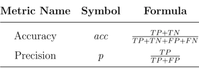
3.5.2 Accuracy . . . 52

3.5.3 Precision and Recall . . . 52

3.5.4 F-score . . . 53

4 Results and Application 54 4.1 Asset Performance Data . . . 54

4.1.1 Preprocessing . . . 55

4.1.2 Preliminary Modeling. . . 57

4.1.3 Indicator Development and Selection . . . 59

4.1.4 Performance Comparison of Failure Prediction Models . . . 62

4.2 NASA Benchmark Data . . . 65

4.2.1 Results. . . 67

5 Conclusion and Future Work 69 5.1 Conclusion . . . 69 5.2 Contributions . . . 70 5.3 Future Work . . . 71 5.3.1 Model . . . 71 5.3.2 Software . . . 71 viii

Bibliography 72

Appendix 88

A Asset Performance Data 89

A.1 Addressing the imbalance problem. . . 89

A.2 Failure indicators . . . 90

Vita 91

List of Tables

2.1 Summary of traditional methods using prognostics and health management . 19

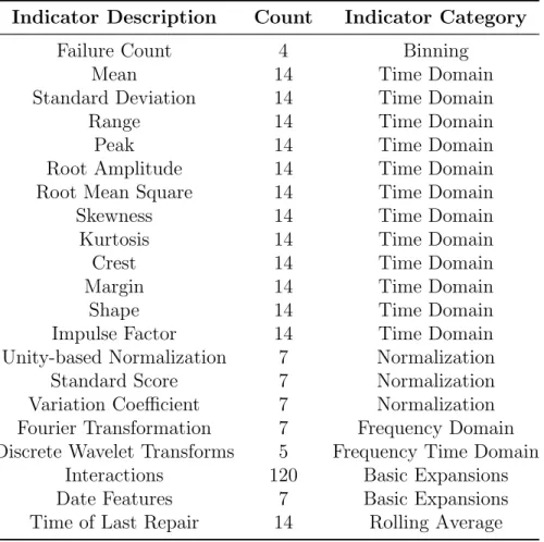
3.1 Summary of Failure Indicators Developed. . . 39

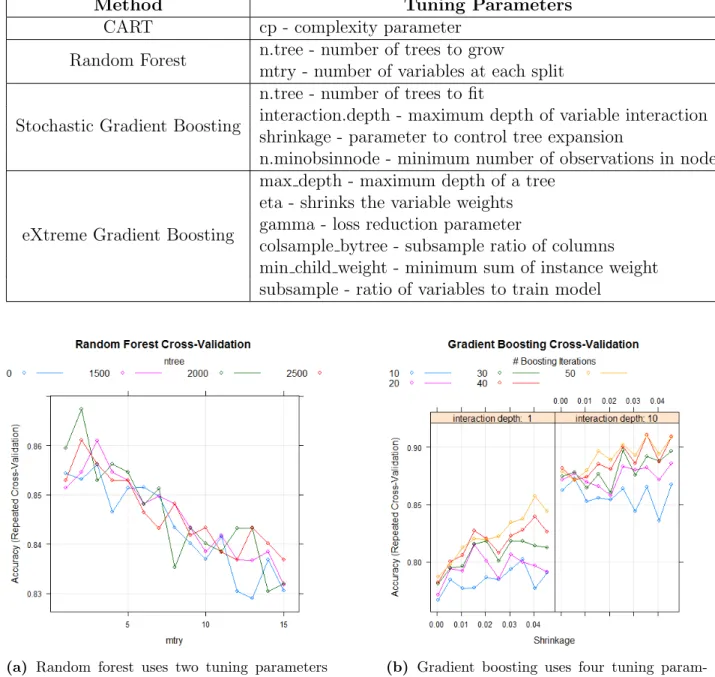
3.2 Tuning parameters for the methods used on training dataset . . . 50

3.3 Confusion Matrix . . . 51

3.4 Metrics derived from confusion matrix (Table 3.3) . . . 52

4.1 Variable description . . . 56

4.2 Description of top 20 indicators selected using random forest model . . . 63

4.3 Performance of the failure prediction methods . . . 64

4.4 Performance of the failure prediction methods for engines . . . 67

List of Figures

1.1 Approach: First, the indicators are developed and passed through filters. Second, the model is built using the indicators. Third, the model is used on

testing data to predict the probability of failure . . . 7

1.2 Framework of the thesis . . . 12

2.1 Classification of prognostics approaches . . . 20

3.1 Methodology Flowchart. . . 29

3.2 Guidelines for model selection . . . 41

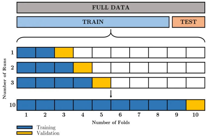
3.3 10-fold cross validation process for time series data . . . 49

3.4 Tuning of random forest and gradient boosting methods . . . 50

4.1 Sensors installed in centrifugal pump to monitor performance, adopted from Meridium(2017) . . . 55

4.2 Centrifugal pump sensor measurements . . . 58

4.3 Performance of preliminary model . . . 59

4.4 The process of creating failure indicators from the historical sensor data in the database . . . 60

4.5 The process of creating failure indicators from the historical sensor data in the database . . . 61

4.6 Comparison of performance metrics and computational time . . . 64

4.7 Engine sensor measurements . . . 65

4.8 Failure in the components . . . 66

4.9 Right:Results of failure prediction models using evaluation metrics accuracy, precision and f-measure. Left: Comparison of computation time . . . 67

A.1 Over-sampling failures to balance the data . . . 89

A.2 Sample of indicators developed from sensor measurements . . . 90

Chapter 1

Introduction

1.1

Overview

Organizations especially manufacturing industries strive to achieve system performance excellence by providing higher quality products and services with reasonable costs and lead times. Fleischer et al. (2006) stated that the performance of a production system mainly depends on the equipment’s availability and productivity. Essential elements in achieving high performance include identifying and anticipating disruptions in the delivery of products and services.

Disruptions include any unexpected event that will affect the standard performance of the system (Darmoul et al., 2013). In a manufacturing context, disruptions manifest in several ways: material unavailability, unavailability of operators, failure of equipment, production schedule overrides, etc. Reducing disruptions improves worker morale and focus (Aytug et al., 2005; Dal et al., 2000), helps equipment run smoothly, reduces raw material waste, and produces higher quality products (Ljungberg, 1998).

Identification of strategies to the improve performance of a system will depend on the critical factors causing the disruptions. Ahmad et al. (2003) listed the most important sources of disruptions in the manufacturing environments:

ˆ Personnel

ˆ Materials

ˆ Schedules

ˆ Equipment Personnel

Personnel include operators and their skills required to work with equipment, it is considered as a critical factor as operators and equipment are in direct contact within in an environment (Miller, 1953). Personnel is influenced by human error and further affects the performance of a system. Most companies have stated that 8% of the disruption are caused by personnel (Gertman and Blackman, 1994), but the source of causes go beyond just human error. If manufacturing industry is embracing the new technology and advancements, then the technology must be practiced in a manner that imports confidence. However, the industries practice different methods, lagging behind in the skills to operate the technology results in disruptions. Some of the personnel disruptions are inevitable as they can occur without any warning during or after the operation of an equipment (Hopp and Spearman, 2011).

Materials

Materials refers to inventory comprising of raw materials, semi-finished material and finished goods at the work stations in a manufacturing line. The stock pile level of inventory correspond to the continuous operation of manufacturing line, if there were no inventory of raw materials at the start of manufacturing line, the shortage will disrupt the normal working condition leading to unscheduled downtime and reduce the performance of the system (Sawhney et al., 2010). Jeziorek (1994) suggested that the high inventory level may address the unscheduled downtime, however, they don’t completely get rid of them. Multiple Japanese methodologies were testing to satisfy the inventory requirements but they were sensitive to variations resulting in a fragile process (Bennett, 2009), where the performance of the system decreased.

Schedules

Scheduling comprises of the process of planning, controlling and scheduling work or workloads in a production process. The planning process allows the organization to allocate resources like personnel and inventory to the required machinery or plant to optimize the productivity (Choi, 1997). The concept of scheduling helps improve the production efficiency by optimizing the manufacturing time and costs. On the other hand, disruptions in the operation schedule results in low levels of inventory which would lead to bad performance of the system.

Equipment

Typically manufacturing environments are subjected to one or more disruptions due to their dynamic nature. The disruptions mentioned above are referred to as real-time events, which can arbitrarily change system status and degrade its performance (Gholami et al., 2009). Equipment disruption is a key factor in the performance of the system which leads to different kinds of breakdowns, and equipment breakdown results in 80% of the downtime in manufacturing systems whether it can be controlled or not (Jabal Ameli et al., 2008). Some of the equipment breakdowns result in disruptions are power outages (Wu et al., 2008), short on equipment consumables (Hopp and Spearman, 2011), failure of equipment (Godinho Filho and Uzsoy, 2011), equipment tools goes out of adjustment (Veeger et al.,2010), tools wearing out (Hopp and Spearman,2011), etc. This research seeks to identify which indicators contribute to system disruptions in the critical bottleneck area and therefore help organizations perform at higher levels by eliminating disruptions with improved equipment reliability and throughput.

The biggest problem equipment disruptions cause are truly unplanned equipment breakdowns. The breakdowns may occur at any point of time in the job, during or in-between them. In August 2001, a crude distillation unit malfunction in the Citgo Petroleum Co. resulted in shutdown of the refinery for 12 months, and estimated total value of loss of $230 million (Marsh, 2014). Failure of a pump in an oil refinery in West Texas led to a

massive fire explosion incurring a loss of over$380 million and shut down for a year (Marsh, 2014). According to a study by Emerson (2016), unplanned outages in data centers results in a loss of nearly $9000 per minute. An analysis by Tucker et al. (2013) of 190 US Gulf of Mexico asset producers in Ziff’s Energy Group revealed an opportunity to improve the production efficiency by reducing the downtime. Total (planned and unplanned) production efficiency of these assets was 88%. Out of the 12% efficiency loss, 8% was relatively caused due to unplanned maintenance. If this loss were prevented, the organization would have saved close to $600 million per year. It is challenging to analyze and repair the equipment within a short period for a human being during the unplanned maintenance since the disruptions are unpredictable resulting in long downtimes. Further leading to fragment loss, facility failures and operational upsets. Therefore, if the breakdowns were known in advance, the organizations can avoid the costly downtimes.

Equipment disruptions can cause unplanned delays in the production process. The delays result in downtime affecting the planned schedule; the process takes extra time than previously planned. Unplanned events like downtime negatively effect the intended capacity’s ability to meet the demand (Melnyk,2007). The delay in one piece of equipment affects the entire process and creates variations in the performance of the production process. Variations caused by equipment breakdowns can be minimized if breakdowns can be anticipated and corrective measures are applied in time. Therefore, when the effects of breakdowns are previously determined, it is possible to develop a methodology to predict the breakdowns and schedule a planned maintenance to reduce downtime. By doing this, high reliability and targeted performance of the system can be achieved.

Planned maintenance results in reliable and safe to operate equipment, therefore influencing the quality, manpower, material, tools and cost (Pintelon and Gelders, 1992; Ahuja and Khamba, 2008). Albino et al. (1992), Savsar et al. (1993) and Vineyard and Meredith(1992) developed simulation models to study the relationship between maintenance and production, and identified the different effect of planned versus unplanned maintenance strategies. Planned maintenance strategies resulted in optimal inventory level and satisfied demand when compared unplanned maintenance, which failed to meet demand. Mosley

et al. (1998) developed a predictive model with the objective to reduce equipment downtime by scheduling maintenance and obtained 20% increase in production. Therefore, planned equipment maintenance is a vital step in the manufacturing process (Ahmad et al., 2003). The literature study shows that mathematical models have been developed to setup planned maintenance activities that mitigate the effect of downtime between the process. Such improvements can be achieved through transitioning from unplanned to planned maintenance.

The motivation behind planned and scheduled maintenance is to improve equipment health, or at least system reliability. It is a vital part of the asset management. Moreover, planned maintenance if done efficiently with proper policies may reduce equipment downtime and other undesirable effects of downtime. Maintenance evidently affects equipment components and its reliability: if little is performed, this may lead to expensive failures and higher downtime, and therefore, reliability is low; performed often, reliability will improve but will result in a linear increase in maintenance cost (Endrenyi et al., 2001).

In a system, if the maintenance is focused on the right equipment at the right time, then a significant impact is made regarding system reliability. Especially if the equipment is the bottleneck of the system, planned maintenance focuses on decreasing downtime by improving the component availability. Taking care of the bottleneck equipment improves the system reliability, production costs are cut, buffer inventories are cut, effective capacity is increased, and moreover, a significant improvement is made in the throughput.

1.2

Problem Statement

Traditionally maintenance practitioners used failure rates, mean time to failure, vibration measurements, oil analysis and a variety of other models which predict failures, but each one of them requires a particular set of equipment. This thesis examines sensors that are typically measured to monitor and evaluate the health of pumps. The sensor measurements are analyzed instead of the failure rates, and a model is developed to predict failure allowing unplanned maintenance to transition into planned maintenance. Sensor measurements

themselves are not sufficient, and therefore, will be modified to obtain relevant information and then filtered bringing the leading and lagging indicators. This is used in the machine leaning models to predict failure rate in centrifugal pumps at a very high probability. The reduction in failure rates using planned maintenance will result in higher reliability of the equipment. This potentially will help eliminate the bottleneck equipment in the process leading to improvement in the throughput of the system.

1.3

Approach

The variables utilized in this thesis were obtained from an extensive database within Meridium (2017), an asset performance management organization. The database consists of a combination of equipments records and its sensor readings at hourly intervals. The equipment considered for research is centrifugal pumps with seven sensor measurements: suction pressure, discharge pressure, flow, temperature, power, rotations per minute (rpm), and vibration.

With the extensive amount of data available and limited data-driven approaches, machine learning models chose the ideal method to be used on the sensor data. Initially, a pilot model is developed using the raw sensor measurements to predict failure. However, the raw sensor data did not contain quality information to predict failure accurately. Therefore, indicators were developed which consisted of encoded information from the raw sensors that improves the machine learning methods to classify the failures (Anderson et al., 2013).

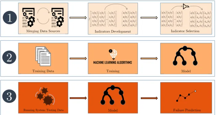
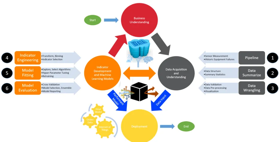
For the methods to work at peak performance and obtain high accuracy, development and selection of the indicators is an important step. The methodology to develop indicators from the sensor data, and build good prediction models using these indicators, as applied here, consists of three steps (see Figure 1.1).

The approach as shown in Figure 1.1 is briefly explained followed by a detailed explanation. The first step in the failure prediction methodology involves development of failure indicators which requires merging the different data sources. This data is used to engineer new leading and lagging indicators that relate to the working condition of

Figure 1.1: Approach: First, the indicators are developed and passed through filters. Second, the model is built using the indicators. Third, the model is used on testing data to predict the probability of failure

an equipment and the best indicators are selected for prediction using filter and wrapper indicator selection methods. In the second step, a machine learning algorithm is trained using the data obtained from the selected indicators. The third step includes the training process which optimizes the objective function and regularizes the model parameters. Since the data sources are historical, the data set is divided into training and testing dataset, where the training data will be used to choose the best model parameters while the testing dataset will be used to evaluate the prediction quality of the algorithm. The tuned and trained model will be later used to predict failures.

The first step is the most important step and the most time consuming, as domain specific knowledge is required for data acquisition, merging it, cleaning and data wrangling, and many iterations of indicator engineering go into it. Specifically, the raw data is imported from three different sources: equipment records, failure and maintenance history and sensor measurements data. The data sources include sensor reading data collected from centrifugal pumps, as well as failure-prone historical maintenance and repair records that detail failure

description and type. The data sources are combined using spatial and time relationship between equipment and sensor readings. Next, the failure indicators are developed; they relate to the working condition of equipment and failure patterns. The indicators obtained from the raw data may not be directly useful or relate to the equipment. Hence, in this case, new indicators or a set of indicators holding the same information as the historical sensor measurements are developed to obtain the leading and the lagging indicators. Sensor data is tagged with a timestamp which helps to calculate the lagging indicators. Some of the indicators developed are:

ˆ Binned indicators

ˆ Frequency domain indicators - Fast Fourier Transform

ˆ Time domain indicators - mean, standard deviation, range, peak, etc.

ˆ Normalized indicators - standard core and silly pins

ˆ Time-Frequency indicators - wavelet transforms

ˆ Lagged indicators - lagged rolling average

ˆ Interaction indicators

Other indicators include a non-linear combination of primary indicators and decomposi-tion transforms. However, not all the indicators are effective enough to predict the failure at a certain stage, and the irrelevant indicators will induce higher computational time. Therefore, important indicators are selected using random forest with specified iterations by optimizing the error parameters and obtaining the importance of each indicator.

When the dataset is preprocessed, and the important indicators are obtained, the next step in the methodology is to select a machine learning algorithm and train an appropriate model. The dataset from the previous step is divided into training and test dataset, where the training data is used for model development, and the testing data is used to evaluate the model. Since the dataset is timestamped data, regular k-fold cross-validation will result

in overfitting the model. Therefore, a time-dependent splitting strategy is used to get a cross-validation statistic and obtain the testing data that are subsequently compared to the training period (Arlot et al., 2010). The approach for selecting the model depends on the equipment iterating failure patterns. These failure events are triggered by the dependency of equipment on the succession of other error events, but not all these events lead to failure. After researching the different mechanisms and dependencies, the following reasons were considered in selected a failure prediction model:

ˆ Equipment health depend on the change in error patterns

ˆ These error patterns have innumerable conditions, where some patterns relate to the equipment leading to failure, and some are just false positives

ˆ To learn and record those patterns which result in failure

ˆ The machine learning techniques are used to train the model based using the recorded patterns

Decision tree learning algorithms such as boosted trees and random forest classifier have been proved to be effective in pattern recognition tasks like automatic recognition of handwritten letters (Polikar, 2006), human emotions (Horn, 2001) and fraud detection (Bishop, 2006). The above being one of the reasons to choose decision tree learners and the second reason being able to differentiate between miscued events, failures and non-failures. Miscued events go unobserved but later deteriorate and become failures which can be detected. This action can be compared to the functioning of tree classifiers in decision trees; the initial states can go unattributed but are later dynamically introduced to the lower stages of the tree structure. The probability of occurrence of failure is predicted by learning the different stages down the line of the decision tree.

The objective of decision learning algorithms is to regularize the hyper-parameters to learn the patterns that lead to failure. To treat the imbalance of classes, i.e., failure and not failures, oversampling techniques are used along with tuning the classifiers to handle the

data. The indicators behave capriciously at different points of time when a failure occurs. Therefore, separate trees are developed in the decision trees to learn the various scenarios of failure sequences. In the prediction phase, the model learns all the different patterns using the training dataset.

The final step of the methodology is to select the best model. Since the failure dataset faces the imbalance problem, various classification evaluations are compared to the benchmarked metrics which are calculated at different scenarios. The comparison of the models using evaluation metrics will help obtain the better performing decision tree model resulting in the accurate prediction of failures. Also, the models are stacked together by combining the outputs using ensembling. Ensembling is relevant when there is a chance of model over-fitting or under-fitting.

1.4

Assumptions

After examining the equipment and sensor records, some characteristics have been deter-mined which result in assumptions based on which the failure indicators and prediction model are developed. The assumptions are:

1. The number of records for failure is less due to rare occasion of failures. The period from the end of failure to the start of next failure is assumed to be non-failures and the sensor records as labeled appropriately.

2. The duration of failure is unavailable in the dataset. Therefore, the end of the maintenance period for that equipment is assumed as the end of the failure period. 3. The equipment running for an extended period and multitasking can sometimes result

in sudden increase or decrease in the sensor measurements. For this reason, such scenarios are assumed to be noise in the data.

4. All the data sources are timestamped. The sensor data contains hourly interval timestamp with sensor measurements while the failure and maintenance records have

timestamp corresponding to the event. It is assumed both the timestamp and indicators contain information to predict failure.

5. Due to the complexity of equipment, it is assumed that the failure patterns at different points of time are different, i.e., different indicators can react to different types of failures resulting in various failure trends.

6. The sensed measurements contain hidden information. Therefore, multiple indicators are developed assuming that all of them are significant. In the following stage, indicator selection is used to identify important indicators.

1.5

Organization of Thesis

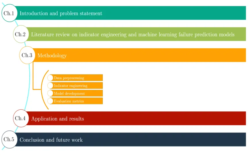
An outline of the thesis is shown in Figure 1.2. Chapter 2 presents the literature review to understand the indicator development and a survey of failure prediction models. Chapter 3

discusses the theoretical details of the methodology that will be used in this thesis. Chapter

4 discusses the results of the methodology applied to the Meridium’s and NASA’s data set. The first dataset is a technical data obtained from Meridium with centrifugal pump records, while the second dataset uses the aircraft turbine engine dataset obtained from NASA’s prognostics center of excellence repository. Chapter 5 includes the conclusion remarks and an outlook to future work.

Figure 1.2: Framework of the thesis

12 12 12

Chapter 2

Literature Review

Compared to the traditional approaches like breakdown maintenance and preventive maintenance, prognostics is still a new field being investigated. In fact, researchers studying prognostics tend to focus on specific areas instead of the field as a whole, mentioning, monitoring, fault detection and diagnostics while disregarding greater possibilities of the field (Heo, 2008; Keller et al., 2006; Liao et al., 2006). Lately, new methodologies and studies have been published for prognostics approaches, which are discussed in detail in the sections that follow.

This chapter discusses the concept of prognostics, different types of maintenance and its undesirable effects. The relationship between real-time sensor data and failure detection is also addressed. The literature relating to the various machine learning methods used for failure prediction, with an inclination towards maintenance management, are also examined in detail.

2.1

Maintenance Management Evolution

Maintenance is defined as “set of activities required to keep physical assets in the desired operating condition or to restore them to the best optimal condition” (Heo,2008;Liao et al., 2006; Pintelon and Parodi-Herz, 2008). In other words, maintenance is a significant factor

that impacts the availability and reliability of the asset to overcome the increase in failure rate which degrades the production quality and efficiency.

Early in the 1980s, maintenance costs summed up to more than $600 billion in the domestic plants in the United States, just to maintain their critical equipments. These costs doubled by the 2000’s (Fluke,2007). Moreover, in some industries like mining, petrochemical, and construction, one-third of the maintenance costs is spent on ineffective maintenance and exceeds the operational costs (Eti et al., 2005;Parida and Kumar,2006).

Over the years, maintenance has expanded from an everyday function into a complex task. Maintenance has undergone a continuous change in the organizational level with increasing complexity of industrial technology and machine tools leading to an elevation in maintenance costs (Parida and Kumar, 2006). Initially maintenance did not receive the importance it deserved, but it evolved to become a major task to increase throughput, mainly by reducing downtime of equipment.

Maintenance evolved from a focus on breakdown and progressed to preventive main-tenance. Eventually, reliability-centered maintenance was developed and advanced to a more practical approach based on condition-based maintenance. Currently, the newest maintenance is based on the prognostics.

The first type of maintenance introduced was breakdown maintenance, where actions are performed after the equipment has come to a complete stop or has become unstable. The equipment was checked for defective parts and repaired. Initially, breakdown maintenance was created only for non-repairable cases and later extended to repairable cases (Barlow et al., 1963).

Multiple types of maintenance actions were defined under corrective maintenance such as minimal repair, general repair, failure replacement and general repair. The researchers have contributed with multiple models which adopted the corrective maintenance actions. The general age replacement model was proposed by Block et al. (1988);Stadje and Zuckerman (1991), in which equipment failures are corrected with minimal repair and returned to their original working condition by identifying the probability repair and replacement.

Among the different corrective maintenance models, one of the appealing models was developed by Kijima (1989) to characterize the equipment and maintenance performances by calculating the new virtual age based on the idea of the primary age. Although corrective maintenance is easy to perform with less work and lower short-term costs, it increases the downtime and reduces the reliability of equipment.

The second concept that was introduced in the evolution of maintenance focused on prevention and originated sometime between the years 1950 and 1960. It was created to avoid a complete shutdown of equipment and disastrous failures. The actions include setting up regular inspections and maintenance at periodic time intervals, regardless of the current condition of the equipment. The critical parameter in PM is determining the optimal time interval for inspection. Savits (1988) and Block et al. (1990) developed one of the first PM models known as a block-replacement model. The model uses fixed time intervals to take action by removing each failure by replacement. Multiple authors (Tilquin and Cleroux, 1975; Boland, 1982; Boland and Proschan, 1982; Aven, 1983) published their work using block-replacement model. Later,Bazovsky (2004) initiated the use of optimization methods in PM models. Jardine and Tsang (2013) used an idea developed by Bazovsky (2004) while developing decision models to calculate the best time interval by extrapolating the historical reliability data and expected cost rate. Kelly (1989) did a survey of practitioners, which proved the unpopularity of fixed time intervals in PM. The strategies in PM reduces the number of failures. However, they do not eliminate immediate disastrous failures between the intervals and also increase maintenance activities, making PM labor intensive.

The evolution of PM was introduced in the late 1960s, when the United States civil aircraft industry developed reliability-centered maintenance (RCM) to reduce cost rate resulting from PM to achieve higher reliability while preserving the functionality of the equipment. It is based on the evolved form of Failure Mode Effect Analysis (FMEA) and involves the use of statistical parameters, particularly probability distributions.

The models in RCM use traditional reliability approaches where the parameters are analyzed based on the distribution of time-to-failure data obtained from similar equipment. The application of RCM using parametric models such as Weibull distributionRausand et al.

(2004), non-homogeneous Poisson process Kothamasu et al.(2009) and Weibull distribution Van Noortwijk(2009) has helped improve the machine reliability. However, the disadvantage is that RCM provides the overall reliability estimate of the whole population of similar equipment in the organization, rather than the real-time reliability estimate of a particular equipment.

In the last two decades, condition-based maintenance (CBM) has been developed in the direction to reduce downtime by monitoring equipment health data without interrupting the normal working operation. CBM introduces maintenance tasks into the schedule only when there is an intervention detected in the measurements observed from the equipment. An able CBM can reduce unnecessary costs by eliminating the scheduled PM tasks. Nonetheless, the minimization of failures and costs require constant on-line monitoring of equipment health. Hess et al. (2008) identified some limitations in CBM traditional methods during a research conference held by National Institute of Standards and Technology, which are described below:

ˆ failed to observe equipment constantly

ˆ inaccurate results in prediction the equipment health

ˆ inability to learn from the historical failure data and detect new failure patterns In other words, CBM methods are limited by inefficiency in observing, reacting, and recommending actions to failures.

As the scope of maintenance gained more importance within the organizational perfor-mance parameters, researchers contributed to enhance CBM’s approach which evolved into the concept of Prognostics and Health Management (PHM) (Hess et al.,2008). PHM can be defined as the ideology in maintenance which integrates the physics of failure mechanism and life-cycle management (Uckun et al.,2008). PHM is today’s most widely accepted practice in high technology equipment based organizations, such as the aerospace industry and military. The United States has allocated special emphasis in this approach within NASA in their spacecraft (Osipov et al., 2007) and the military in two different programs. The programs

are Joint Strike Fighter Program (Hess et al., 2004) and Future Combat Systems Program (Barton,2007) for anomaly detection, efficient diagnostics, real-time performance monitoring and predicting failures.

PHM has been acting its part in the multiple areas helping industries from the equipment manufacturer to the end user. Some of the advantages of PHM compared to the other maintenance systems (Hess et al.,2008; Uckun et al.,2008;Asmai et al., 2010;Balaban and Alonso, 2012) are:

ˆ improvement in equipment reliability (forecast failure-prone equipment)

ˆ ability to recommend maintenance actions to increase life of an equipment

ˆ reduction of downtime and operational costs by elimination of unnecessary maintenance actions

The main contribution of PHM is to provide the end users the knowledge of the future health of equipment. This job broadly consists of two different steps. The first step is monitoring and accessing the health condition; then anomaly detection techniques can be used here to detect various types of failure patterns. The second step aims at predicting the probability of failure, where machine learning methods are used (Si et al., 2011).

In summary, the evolution of maintenance has expanded from simple reactive approaches to data guided prediction, as the nature of business rely on effective strategies. The thesis focus on present day approaches while expanding the body of knowledge regarding PHM.

2.2

Prognostics and Health Management

PHM is a concept within equipment monitoring maintenance system which also includes fault analysis, equipment diagnostics, anomaly detection and online monitoring. Kothamasu et al. (2009) referred to prognostics as the complete form of CBM system. The authors have used PHM estimates to develop applications for maintenance assessment and scheduling. Pintelon and Parodi-Herz (2008); Hess et al. (2008) researched the use of PHM to predict failure for

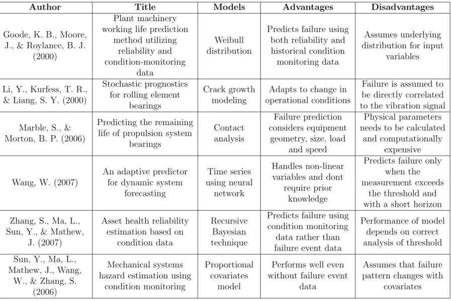
logistics systems. Table 2.1 lists the exciting research work using prognostics and health management.

Callan et al. (2006) divided the PHM system into five different steps: data acquisition, data manipulation, condition monitoring, health assessment and prognostics. Prognostics is the most important measure used to “estimate the time of failure or risk for one or more existing and future failure modes” (Katipamula and Brambley,2005). The application of all the steps in the CBM will result in the improvement in production, reduction in downtime and failures, improved work performance of equipment, elimination of unnecessary downtime and a decrease in life-cycle cost.

The model considers the original data and produces the results in the form of probability of failure to schedule maintenance routines. Data is collected through continuous online observation of equipment and analyzed for pattern changes. The analysis can be performed with the help of different methods, including statistical and empirical models (Ma and Jiang, 2011). The current condition of the equipment is assessed and compared to the estimates of the degradation level; this helps determine if the equipment is operating abnormally. A statistical method utilizes the estimates distribution of normal working and degraded condition to determine the shift. If a shift is observed, it is important to determine the cause; equipment has different degradation levels based on the type of failure. Finally, different prognostics models can be used to determine the probability of failure of the equipment.

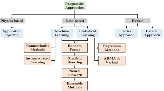
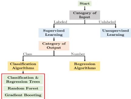
Prognostics algorithms can be classified into three types: physics-based, data-driven and hybrid prognostics as shown in Figure 2.1 (Si et al., 2011).

Table 2.1: Summary of traditional methods using prognostics and health management

Author Title Models Advantages Disadvantages

Goode, K. B., Moore, J., & Roylance, B. J.

(2000)

Plant machinery working life prediction

method utilizing reliability and condition-monitoring data Weibull distribution

Predicts failure using both reliability and historical condition monitoring data

Assumes underlying distribution for input

variables

Li, Y., Kurfess, T. R., & Liang, S. Y. (2000)

Stochastic prognostics for rolling element

bearings Crack growth modeling Adapts to change in operational conditions Failure is assumed to be directly correlated to the vibration signal Marble, S., &

Morton, B. P. (2006)

Predicting the remaining life of propulsion system

bearings

Contact analysis

Failure prediction considers equipment

geometry, size, load and speed Physical parameters needs to be calculated and computationally expensive Wang, W. (2007) An adaptive predictor for dynamic system

forecasting

Time series using neural

network

Handles non-linear variables and dont

require prior knowledge

Predicts failure only when the measurement exceeds

the threshold and with a short horizon Zhang, S., Ma, L.,

Sun, Y., & Mathew, J. (2007)

Asset health reliability estimation based on

condition data

Recursive Bayesian technique

Predicts failure using condition monitoring

data rather than failure event data

Performance of model depends on correct analysis of threshold Sun, Y., Ma, L.,

Mathew, J., Wang, W., & Zhang, S.

(2006)

Mechanical systems hazard estimation using

condition monitoring

Proportional covariates

model

Performs well even without failure event

data

Assumes that failure pattern changes with

2.2.1

Physics-based Prognostics

The physics-based algorithms for prognostics use mathematical techniques to model and understand the degradation of equipment (Pecht and Jaai, 2010). The equipment health estimates using this algorithm are based on the process information that causes abnormal activity and results in failure. They detect failure which occurs under the circumstances of mechanical, electrical, chemical, thermal and radiation disturbances (Pecht and Gu, 2009). The algorithm is selected based on the knowledge of loading conditions and equipment geometry (Pecht, 2008).

Figure 2.1: Classification of prognostics approaches

Physics-based prognostics are developed with an application in specific and applied at the lowest hierarchy. Heng et al.(2009) suggested that physics-based methods are inefficient to use in an industrial environment, because of the different types of failures observed in various types of equipment. Furthermore, method selection is hard when the geometry of the equipment is unavailable (Pecht and Jaai, 2010). Therefore it is ineffective to use this due to the various assumptions, errors, and uncertainty developed in a dynamic operating condition which leads to lower accuracy (Wang, 2010).

2.2.2

Data-driven Prognostics

Data-driven approaches develop models based on the condition monitoring data instead of models that depend on the comprehensive equipment physics. They assume that unless an abnormal activity occurs in the system, it keeps working in normal condition. This approach obtains relevant information from the raw data and behavior patterns of the equipment. Therefore, data-driven methods have a better application due to economic modeling, as they depend only on the historical data and don’t require any human expertise (Javed et al., 2013;Pecht and Jaai,2010). The data-driven prognostics methods are classified into machine learning and statistical approaches.

Machine learning methods are based on the concept of artificial intelligence. They learn from previous examples of failure patterns and modes in historical data. Based on the types of data available, different types of machine learning methods can be applied. Supervised methods are used when the data is labeled, while unsupervised methods are applied to unlabeled data. Atherton (1999) and Yam et al. (2001) developed prognostics model using recurrent neural networks (supervised method) to analyze the trends in the monitored data and forecast the equipment measured value for the future. Zhang et al. (2007) used a recursive Bayesian method on density function of measured values from the equipment to predict failure probability. The model mostly used historical degradation pattern rather than the failure event data.

Statistical approach predicts failure by fitting the monitored data to a probabilistic model, and fitted curve is extrapolated. Statistical methods are similar to machine learning methods: they are simple and use the condition monitored data to predict failure. However, the accuracy of the model can depend on the completeness and nature of data. Si et al. (2011) presented a survey of a literature review of statistical methods. The survey list includes multiple methods such as regression methods, Hidden Markov models, Kalman filtering methods, etc,. Orchard et al. (2005) employed a particle filtering method to forecast the non-linear projection of increasing degradation in the turbo engine blade. A priori estimate

was calculated based on the previous state of the blade and used to generate the prediction horizon of the desired state.

Data-driven prognostics have the ability to extract relevant information from big noisy data to make prognostics decisions (Dragomir et al., 2009). When data is collected from equipment operating in a real industrial environment, it contains variability and noise. Therefore the preprocessing step is an essential step to extract relevant information to improve the accuracy of the model.

2.2.3

Hybrid Prognostics

Hybrid prognostic is a combination of physics-based and data-driven approaches. The significance of this method is to develop an optimized prognostics model using both historical monitoring and reliability data with minimal assumptions to handle uncertainty and predict failures of high accuracy. Sun et al. (2006) proposed proportional covariates model (PCM) which used system hazard as an explanatory variable and the monitoring data as response variables. This model was used to estimate the hazard function in the absence of historical failure data as long as the response variables were proportional to the hazard. Further research suggested that both event failure and condition monitoring data was used in measuring reliability estimation parameters. Hybrid prognostics is further divided into two types: series and parallel approaches. In a series approach, a physics-based model is paired with the data-driven method to update model parameters with new training data (Psichogios and Ungar, 1992). In a parallel approach, a combination of data-based and physics-based models work in concert to predict residuals in situations when other models cannot (Thompson and Kramer, 1994).

Heng et al. (2007) developed a new paradigm called intelligent product limit estimator which incorporated data composed of equipment health up to the time of repair or replacement (suspended or truncated data) to predict failure. The model built using the suspended data resulted in an excellent long-range prediction, as the equipment in operation are never allowed to run to failure and data are suspended. In the model, Kaplan-Meier

develops estimates using the variation in equipment health, and these estimate probabilities are used as training targets in the feed-forward neural network. The research presents a model which utilizes the available information and provides accurate prediction in a probabilistic unit.

Despite the abundant research efforts, prognostics approaches are not perfect due to the assumptions inherent in every model (Sikorska et al., 2011). Furthermore, each approach has pros and cons, while limiting their application on the data available. A prognostics approach for a particular application is selected based on two important factors: performance and applicability (Jardine et al., 2006). Javed (2014) compared all the three prognostics approaches by assigning weights based on different criteria in performance and applicability. The data-driven approach had the maximum weight in the applicability factor as it can learn various types of failure patterns with its general methods. However, it requires improvement in the performance part. An et al.(2015) compared all the approaches with the help of case study, and data-driven method outperformed others with machine learning methods. The data-driven method performs better in the event of high levels of noise and large training data sets. Machine learning methods in data-driven approach is still an improving field, but it is heavily researched to improve some of the drawbacks. Because data-driven approach especially machine learning methods are the most efficient with good applicability, this method will be considered for further analysis in the thesis.

Some machine learning methods obtain high accuracy and some fails (Domingos, 2012), while the quality of the data has a big impact on the performance of the learning algorithm too. Inconsistent data will reduce the efficiency of a well tuned complex algorithm, while a good dataset can obtain high accuracy using a simple algorithm. Thus, developing features from raw data to extract the useful information is important (Domingos, 2012). It is also important to note that adding useless features to the data will result in overfitting the machine learner. Hence, in this study, the drawbacks are addressed by introducing a method to develop indicators of importance and selecting them to prevent curse of dimensionality.

2.3

Sensor Technology in Maintenance

Prognostics approaches have a long history of methods which evolved from using visual inspection to sensor signals to predict failures. Traditionally human interaction was required to diagnose equipment degradation. Fortunately, sensor technology has taken over the advanced maintenance approaches to help identify failures (Spencer et al.,2004). Utilization of sensor signals in parallel with the prognostic approach based data-driven methods will reduce unplanned maintenance costs, and improve availability and safety.

In spite of advancement in maintenance technologies, unplanned and hand-held based maintenance is still being used in some industrial equipments. At present, nearly 30% of the equipment is not using modern technology in maintenance practices (Hashemian et al.,2005). Emerson company reported the dataset containing pressure, level and flow transmitters measured using hand-held maintenance technology in multiple industries. Emerson found that 70% of the time maintenance was scheduled based on the measurement reading, while there was no breakdown in the transmitters (Hale, 2007). However, some nuclear plants utilized online sensor technology to get sensed reading and found that there were no problems 90% of the time in equipment (Hashemian et al., 1998). The above literature suggests that online sensor technology, rather than hand-held devices, reduces the failure rate and downtime.

Hashemian et al. (1995) describes that in online calibration monitoring, the equipment with sensor measurements drifted beyond the control-limits was identified and maintenance actions was performed during the plant downtime. This approach minimized the efforts of operators by 90%. Hashemian et al. (2005) developed the loop current step response method, which used active sensor measurements to schedule planned maintenance in cables, motors and thermocouples. As noted by Hashemian et al. (2007), sensor-based predictive maintenance methods were used to detect blockages in pressure sensing lines with the help of pressure sensor placed at the end of the sensing line.

Effective sensor technology and monitoring builds a good foundation for developing an efficient prognostic based maintenance. In fact, the data generated from sensors are a critical

component for prognostics approach. However, the options of how the sensor data can be utilized is still being researched. The sensed data is collected from different sources which are not interconnected and an independent model is built for each source (Levis et al.,2004). With improvement in sensor technology, integrated online sensor monitoring systems were developed, but still lack the automated failure prediction model to utilize them efficiently (Madria et al.,2014). Therefore, this thesis discusses the ways to close the gap of automation using machine learning methods to build an automated failure prediction model.

2.4

Failure Prediction Models

The primary motivation for the development of prediction models is to understand the effect of the quality of historical data on the decision that help schedule planned maintenance to prevent failure in equipment. The failure event data and condition monitoring data can be efficiently utilized to identify failure patterns of different faults in equipment and guide maintenance decisions so as to reduce failure and downtime. In this section of the chapter, different machine learning techniques that can be used in the prediction of failure is discussed. Recently there has been a significant increase in the use of predictive models in prognostics methodology. Multiple models have been developed for specific equipment or type of failures. The methods include random forest, gradient boosting, neural networks and ensemble learning methods. The focus is based on data-driven prognostics in the development of failure prediction models and moreover, to compare the performance to select the best technique for the study. The methods selected in this study were influenced by the application in a specific environment, the quality of historical data, predictive performance and computational requirements for applicability of the method.

Random Forest

Recently, random forest (RF) as a machine learning technique, has been utilized for failure prediction in multiple operations of engineering due to its robust ability to work efficiently with large number of indicators, small samples and also its simplicity in interpretation of

tree-based models (Timofeev, 2004; Verikas et al., 2011). RF uses a tree-based classifier (Breiman et al., 1984a), integrated with bootstrap aggregation (Breiman, 1996). The algorithm exploits the use of trees in the method. Each failure pattern is trained in isolation in a tree, and the predictions of all trees are combined to get a sophisticated result. Using this method, Frisk et al. (2014) have predicted failures in lead-acid batteries with training data obtained from heavy duty trucks containing heterogeneous data of 300 variables. RF performed well even with imbalanced and missing data from trucks.

Santur et al. (2016) proposed the use of RF in a study to predict the failure that may occur in railway tracks. Video image data of railway tracks was used to extract indicators, and the data was used to predict the different types of faults like scouring, breaking and deficient fasteners on tracks. The three different methods: principal component analysis, singular value decomposition, and random forest were compared with RF achieving the highest accuracy of 85%. In the study health assessment of bearings, Satishkumar and Sugumaran (2016) used vibration signals of bearing to develop a failure prediction model using RF. An accuracy of 95.64% was obtained by initially performing a feature selection using decision trees.

Gradient Boosting Method

Friedman(2002a) developed gradient boosting machine (GBM), a machine learning classifier to improve the predictive performance in classifications. GBM is highly appreciated because of its robustness to interactions, missing values, imbalance and outliers (Hastie et al.,2009). Furthermore, it automatically selects variables and leaves out irrelevant variables.

Kelvin (2016) analyzed the occurrence of unexpected failures in 1100 automated teller machines and 280 cash acceptance machine. Multiple models were used in the modeling step, and GBM resulted in the best model with an area under the curve of 87% to predict the failure. Furthermore, there were key challenges of data format and volume which was efficiently handled by GBM. Cerqueira et al. (2016) faced multiple challenges with the air pressure system components from Scania trucks. There were missing values, outliers and imbalance in class distribution. IN this situation, GBM was selected as the best method to

handle the challenges and prevent overfitting. Two different algorithms, random forest and extreme gradient boosting, were used to model the failure of air pressure components. The best model (extreme gradient boosting) was generated with parameter tuning using ten-fold cross-validation and obtained sensitivity cost of 3750 and lowest deviance.

In contrast to using raw sensor variables as training data and traditional statistical methods in Hu et al. (2016) and Liu et al. (2016) to predict failure, this thesis aims to develop relevant leading and lagging indicators from sensor variables that contain useful information to explain the failure patterns in equipment. The best subset of indicators are selected for modeling using the random forest and gradient boosting methods. The best failure prediction model is selected based on their applicability to utilize the indicators developed from the equipment and metrics in performance assessment. The following chapter will discuss the methodology followed in this research along with a detailed explanation of all the methods used.

Chapter 3

Methodology

This chapter describes the methodology developed to attain the objectives of the thesis. Initially, indicators are developed utilizing the historical dataset, and they are used in the machine learning algorithm. The details of the development of indicators and working of machine learning are discussed in the section of this chapter in detail. The methodology has been divided into the following phases:

1. Data preprocessing 2. Indicator development

3. Model development and selection 4. Evaluation metrics

The data preprocessing phase consists of a novel approach to clean and prepare the data for modeling. Indicator development describes the techniques to develop the leading and lagging indicators. The model development phase consists of the mathematical formulation and techniques used in formulating the machine learning algorithms for failure prediction. The evaluation metrics phase describes the different evaluation strategies for analyzing the quality of the prediction results.

3.1

Data Preprocessing

Data preprocessing is the phase in the methodology where the data is prepared for further use in modeling. The challenge in this phase is the number of different activities it involves, including variable parsing, outliers checking and balancing the label variables. Due to an improvement in infrastructure, sensor measurement reliability increased linearly over the last decade when compared to antiquated, manual models of data processing. Therefore, preprocessing is a necessary task required for the model to predict failure accurately.

3.1.1

Data Organization

According toWickham et al.(2014), the first step is to map the dataset to match its structure, which is performed by the following steps:

1. Each variable is allocated to its unique column 2. Each observation is allocated to its unique row

3. Each observational unit is assigned to its unique table

The above steps result in a standard structured data that is easier to read because the structured layout form paired values from different columns with the same row. However, it does not affect the further analysis which demands organization of the variables. The most efficient way of organizing the variables is by their importance in the analysis; the fixed time stamp variables should come first followed by the measured sensor measurements. Rows are then sorted based on the time stamp variables, cutting off ties with other fixed variables.

The data structuring step is followed by tidying the dataset read to the system. Initially, the dataset requires further preparation before jumping to the analysis part. Wickham et al. (2014) pointed out the most problems in messy datasets:

1. Column header has random names, not variable names. 2. Multiple information is stored in the same column

3. Variables are stored in both rows and columns

Commonly the messy dataset is arranged with values of the row and column rather than the variable names. This arrangement of data might sometimes prove useful for efficient storage and computation, but it complicates the analysis process failing to recognize the uniqueness of the variable. To improve the identification of variables, the values in the headers are converted to columns with a unique variable name. The names allocated to the columns based on the variable are easy to use and informative, maintaining the consistency throughout the dataset.

Often, after converting values to variable names, there are multiple variable names in the same column. The variable names in this format can be further broken down to form additional variables, which results in useful information. Preprocessing the data in this form extracts the hidden information resolving another problem in the messy dataset.

Variable values stored in both rows and columns is the most tricky part of the preprocessing. The information of a certain variable is spread all over the data across rows and columns making it difficult the analyze. The variable names are stored in the columns while the observation values are the headers. This issue is fixed by reconstructed the data to represent the variable names as the columns headers and each row represented by a sample.

3.1.2

Imbalanced Datasets

In the real world, datasets involving the health of equipment present imbalance in the dataset due to rare instances, i.e., failure, which makes it difficult to develop a model as there is little failure data compared to non-failure data to learn.

Developing a prediction algorithm with an imbalanced dataset results in a high accuracy of the model but the prediction classifier is biased towards majority class as the number of rows with minority class being small. For example, consider an imbalanced dataset with 20:80 ratio of minor to major label classes resulting in an accuracy of 95%. This model initially looks like the perfect model but the results could be deceiving since accuracy favors labels of major classes strongly while the minority classes are being misclassified.

There are a couple of methods to solve the imbalance problem in the dataset. The most efficient method found in the recent literature to re-balance the dataset is Synthetic Minority Oversampling Technique (SMOTE) Chawla et al. (2002). In this approach, the minority class is over-sampled by generating new examples to match the number of majority classes. SMOTE identifies the nearest neighbor of the minority class example using the Euclidean distance. A synthetic example is generated based on two examples and placed randomly somewhere between them.

Data preprocessing is an important phase in the methodology; good quality data improves the end results of the modeling. Like the usual saying garbage in and garbage out, a good quality data input to the model will lead to high-quality prediction output.

3.2

Indicators Development and Selection

Developing indicators is the process of using domain-specific experience and data insights to create features that help in the machine learning prediction. More than one indicator is used at a time in a prediction model; the more uncorrelated the indicators are from each other, the greater the information gain from the indicators. The set of indicators developed for the prediction model is referred to as feature space.

In the application of predicting failures using machine learning algorithms, the data acquired must be preprocessed before the development of feature space for effective results from the machine learning methods (Zhang et al., 2010). Every variable in the dataset is developed into a set of features that defines the feature space. This phase is not only limited to the development of indicators but also includes indicator selection which extracts the most important features affecting the trend of failure.

3.2.1

Indicator Development

Indicator development is based on different techniques that derive the required information from the raw sensor data in order to replace variables with new and better indicators. The

development utilizes functions from various mathematical and modeling techniques to learn from the observed and measured sensor variables. Tan and Jiang (2013) has experimented with techniques like decomposing, filtering, translating and more to extract the hidden information in the sensor data. This thesis uses different techniques to develop indicators using the historical sensor measurements which signify strong statistical evidence between the trend in sensor variables and the occurrence of failures.

Binning Indicators

Binning is a process of transforming continuous variables into nominal or categorical indicators which help in creating density estimations of the measured values. When used correctly, the binning process can improve the simplicity of the model and decrease computation time (Kim and Han, 2000). There are multiple methods in binning but equal width interval binning was used because of its tendency to produce low discretization error. In equal width interval binning, the variables are sorted and divided into k equally sized intervals. For a variablexwith the minimum and maximum values denoted by the xmin and xmax, the bin width is determined by:

δ = xmax−xmin

k (3.1)

The value k is determined by Sturges rule where k = 1 +log2(n), where n equals the length of the dataset (Yang and Webb, 2009). Then the method passes through the entire dataset once transforming each variable into binned indicators independently.

Time Domain Indicators

The trends of the measured variables can vary from time to time presenting non-stationarity in the data. According to Virili and Freisleben (2000), the time-dependent variables with trends can often cause complexity in modeling, leading to a decrease in the quality of predictions. Therefore, the transformed variables can display the clear change in patterns

after removing the variability. In this section different time-dependent functions are used to extract the indicators in the time domain as represented in the equations 3.2 - 3.13.

mean :xm = PN n=1x(n) N (3.2) standard deviation :xstd = s PN n=1(x(n)−xm)2 N −1 (3.3)

range :xr =max(x(n))−min(x(n)) (3.4)

peak :xp =max|x(n)| (3.5) root amplitude :xra = PN n=1 p |x(n)| N !2 (3.6)

root mean square :xrms =

s PN n=1x(n)2 N (3.7) skewness : xske= PN n=1(x(n)−xm)3 (N−1)x3 std (3.8) kurtosis :xkurt = PN n=1(x(n)−xm) 4 (N −1)x4 std (3.9) crest :xc= xp xrms (3.10) margin :xma = xp xra (3.11) shape :xsha = xrms xm (3.12) impulse factor :xif = xp xm (3.13) where, n is the variable values from n = 1,2,3...,N and N is the length of the dataset.

Normalization Indicators

Normalization is the process of transforming the measured values to a common scale to deal with variables of different units and scales. Some of the machine learning methods are prone

to outliers; normalization intends to compare the corresponding normalized values reducing the effects of exceptional values. The different functions used to normalize the variables are:

unity-based normalization :xun = x(n)−min(x(n)) max(x(n))−min(x(n)) (3.14) standard score :xss = x(n)−xm xstd (3.15) variation coefficient :xvc = xstd xm (3.16) Normalization is a tedious process as the future distribution of the variable is unknown, leading to the null maximum and minimum values of the variable. Therefore, normalization is to be performed after binning the variables which will eliminate outliers Gaber et al. (2005).

Frequency Domain Indicators

The frequency domain functions transform a given variable on each given frequency band. Finding the frequency at a particular point in time is irrelevant, but it is important to find how much of that particular frequency is in the variable. These frequency domain indicators are developed to find the distribution of frequency and filter the noise. Filtering in the time domain results in complexity and causes convolution. Therefore, the time-dependent variables are transformed into frequency domain, remove the noise with filtering and transform it to obtain the time-dependent indicators. Fourier transform functions are used in this case to develop the indicators.

Fourier transform treats the values in the variable as a point in the circular path and divides it into a group of cycles that hold the same information as the original variable (Bracewell and Bracewell, 1986). The properties of cycles are defined by strength, delay, and speed which is later used to recreate the original variable. Initially, the variables are passed through filters where each independent filter extract a cycle, i.e., the filters extracts all the values in the variables without leaving any observation. After the filtering, the original variable is obtained from the linear combination of the cycles. Fast Fourier Transform (FFT)

algorithm is selected to perform the transformation and presented by the complexity of O(n.log(n)) operations. The FFT algorithm consists of two equations (Harris, 1978), where equation 3.17 represents the transformation from time domain to frequency domain and Equation 3.18 converts the frequency domain variables back to the original time-dependent variables. Xk = N−1 X n=0 xne−i.2πkn/N (3.17) xn = 1 N N−1 X k=0 Xke−i.2πkn/N (3.18) where,

Xk = amount of frequency k in the variable N = number of samples

n = current sample, n∈ {0, .., N−1} k = current frequency

xn = value of the variable at timen

The transformations result in the development of indicators like frequency peaks in the variable or the rate of change in the certain frequency.

Frequency Time Domain Indicators

The measured variables may contain hidden information in the frequency domain with continuously changing statistics with time; such information can be extracted using the time-frequency analysis. The methods analyze variables in tim