to Generalized Linear Models, Generalized
Additive Models, and Smoothing
Sri Utami Zuliana
A thesis submitted for the degree of
Doctor of Philosophy
Department of Mathematical Sciences University of Essex
ii
Dedicated to
My fatherAyah Djahidand my motherUmi Rus
Acknowledgements
I would like to express my gratitude to Almighty Allah.
There are many people that helped, inspired and encourages me to progress and complete this thesis, to whom I am deeply thankful. First and foremost, I gratefully acknowledge the support of my supervisor, Dr. Aris Perperoglou. He has provided me with his remark-able insights, guidance and continuous encouragement. This work would not have been possible without his help and guiding. I am thankful to my supervisory board member Prof. Peter Higgins for his valuable suggestions and encouragement.
I am very thankful to Ministry of Religious Affair, Republic of Indonesia for financial
support and UIN Sunan Kalijaga, Yogyakarta, Indonesia for full support. I am thankful to the administration of Department of Mathematical Sciences University of Essex for their support.
I would like to thanks to all my friends with whom I shared my happiness and sadness and who helped me during my study. I am thankful for my brother, my sisters in law and all my big family members for their support.
iv
Abstract
Recently, penalized regression has been used for dealing problems which found in maxi-mum likelihood estimation such as correlated parameters and a large number of predictors. The main issues in this regression is how to select the optimal model. In this thesis, Schall’s algorithm is proposed as an automatic selection of weight of penalty.
The algorithm has two steps. First, the coefficient estimates are obtained with an arbitrary
penalty weight. Second, an estimate of penalty weightλcan be calculated by ˆλ= σˆˆ2
τ2, where
ˆ
σ2 is the variance of error and ˆτ2 is the variance of coefficient. The iteration is continued
from step one until an estimate of penalty weight converge. The computational cost is minimized because the optimal weight of penalty could be obtained within a small number of iterations.
In this thesis, Schall’s algorithm is investigated for ridge regression, lasso regression and two-dimensional histogram smoothing. The proposed algorithm are applied to real datasets and simulation dataset. In addition, a new algorithm for lasso regression is proposed. The performance of results of the algorithm was almost comparable in all
applications. Schall’s algorithm can be an efficient algorithm for selection of weight of
Declaration
The work in this thesis is based on research carried out at the Department of Mathematical Sciences, University of Essex, United Kingdom. I certify that this is all my own work, unless referenced in the text, no part of this thesis has been submitted elsewhere for any other degree or qualification.
Copyright c 2017 by Sri Utami Zuliana.
Abreviations
AIC Akaike information criterion
AICc Akaike information criterion with a correction
B-splines basis splines
BIC bayesian information criterion
ED effective dimensions
GAMs generalized additive models
GCV generalized cross-validation
GLMs generalized linear models
i.i.d independent and identically distributed random variables
IWLS iterative weighted least square
Lasso least absolute shrinkage and selection operator
MLE maximum likelihood estimation
MSE mean squared errors
OLS ordinary least squared
P-GAMs generalized additive models with penalized B-splines
P-splines penalized B-splines
Contents
Acknowledgements iii Abstract iv Declaration v Abreviations vii 1 Introduction 12 The Weight of Penalty Optimization for Ridge Regression 4
2.1 Introduction . . . 4
2.2 Ridge Regression in a Generalized Linear Models (GLM) . . . 6
2.2.1 Ridge regression from Bayesian perspective . . . 7
2.3 Simulation . . . 10
2.4 Summary . . . 15
3 Ridge Regression in Poisson Models and Logistic Models 18 3.1 Introduction . . . 18
3.2 Optimized Poisson Ridge Regression and Logistic Ridge Regression . . . . 19 viii
3.3 Applications . . . 21
3.3.1 Example . . . 22
3.3.2 Datasets Simulations for non-correlated covariate . . . 24
3.3.2.1 A non-correlated Poisson regression model . . . 25
3.3.2.2 A non-correlated logistic regression model . . . 25
3.3.3 Datasets Simulations for correlated covariates . . . 26
3.3.3.1 A correlated Poisson regression model . . . 26
3.3.3.2 A correlated logistic regression model . . . 27
3.4 Summary . . . 28
4 Generalized Additive Models 30 4.1 Introduction . . . 30
4.2 B-spline basis functions . . . 33
4.3 Penalized splines (P-splines) . . . 35
4.4 Univariate Smoothing with GAMs with P-splines(P-GAMs) . . . 37
4.5 Optimal Smoothing . . . 38 4.6 Application . . . 40 4.7 Simulation . . . 42 4.8 Summary . . . 44 5 Lasso Regression 45 5.1 Introduction . . . 45 5.2 Definition . . . 46 5.3 Computation . . . 47
Contents x
5.4 The proposed algorithm . . . 48
5.5 Application . . . 50
5.5.1 Simulation . . . 50
5.5.2 Prostate Cancer Data . . . 51
5.5.3 Microarray data set . . . 52
5.5.4 PRIDE models . . . 52
5.6 Summary . . . 55
6 Two Dimensional Smoothing via an Optimised Whittaker Smoother 58
7 Conclusion and future work 63
Appendix 71
List of Figures
2.1 Distribution ofλs based on different methods of optimization . . . 11
2.2 Boxplot of computation time with respect to method for the simulated data
with correlation between the independent variables . . . 13
2.3 Distribution of estimatedλs based on different methods of optimization for
the simulated data with no correlation between the independent variables . 15
2.4 Distribution of computation time based on different methods of optimization
for the simulated data with no correlation between the independent variables 16
3.1 The coefficients of five covariates are shrunk to zero. AIC, BIC, GCV and
Schall’s algorithm give different optimal fit. The optimal coefficients from
Schall’s algorithm (+) (λ = 95.78) are located in the middle of three other
criterions. . . 24
4.1 Scatterplot of the motor-cycle impact data. It can be seen that a simple linear
regression is not the best model. . . 31
4.2 Polynomial regressions are applied to mcycle. It can be seen that as the
degree is higher, the fit is more sensitive. The polynomial regression degree
20 above 50 ms does not represent what happened on the data set. . . 32
List of Figures xii
4.3 Illustration of B-spline bases degree 1 with knot sequencet={0,0.2,0.4,0.6,0.8,1.0}
. . . 34
4.4 Illustration of B-spline bases degree 2 with knot sequencet ={0,0.2,0.4,0.6,0.8,1.0}
. . . 35
4.5 B-spline regressions with different number of knots. Upper left, the fit is
resulted from B-splines with 20 knots. Upper right, the fit is resulted from B-splines with 25 knots. Lower left, the fit is resulted from B-splines with 30 knots. Lower right, the fit is resulted from B-splines with 30 knots. As
bigger the number of knots, the fit is more wavy . . . 41
4.6 The curve is resulted from P-spline with 40 knots. The optimal weight
of penalty of P-spline regression is selected automatically using Schall’s
algorithm. . . 42
4.7 Scatterplot of the simulated data. It can be seen that a simple linear regression
is not the best model. . . 43
4.8 Left: the smoothing result from optimized P-GAM.;Right: the smoothing
result from tensor product (package mgcv). . . 43
5.1 Estimated coefficients under the different packages i.e. glmnet,penalized,
proposed algorithm using grid search, and proposed algorithm using Schall’s algorithm. The proposed algorithm using Schall’s algorithm penalized less
5.2 Upper: A histogram of the number of deaths for Greek males in 1960. Three
smoothers have been applied with PRIDE modelling, usingL2(blue line),L1
(green line) andL0(red line) penalization. Lower left: Plot of deviance effects
underL0penalization, lower middle: deviance effects underL1penalization,
lower right: deviance effects underL2penalization. . . 56
6.1 Optimized Smoother Whittaker . . . 61
6.2 Tensor Product . . . 61
6.3 Optimized Smoother Whittaker . . . 61
6.4 Tensor Product . . . 61
6.5 Otimized Smoother Whittaker . . . 62
List of Tables
2.1 The average prediction error of different methods. . . 12
3.1 The simple Poisson regression results show that all covariate has a
signifi-cant P-values. In column 2 and 3, coefficients and standard errors of each
variables are given. The last column shows that each variable has a
signif-icant P-values (less than 0.001). However, they are highly correlated data.
Opium has a correlation with area (0.48), mountainous has a correlation with all-season roads (-0.65) and acces to drinking water (-0.68), below min-imum calories has a correlation with literacy rate (-0.46), and majority has a
correlation with acces to drinking water (0.49). . . 23
3.2 The average of coefficients of Poisson regression using ridge regression for
non-correlated data. Schall’s algorithm, AIC, BIC, GCV and MLE doesn’t
give different MSE and mean percentage of bias (mpb) value. So the simple
Poisson regression analysis is enough. . . 26
3.3 MSE from non-correlated logistic data for different sample sizes i.e. 400, 450,
475, 500 and 1000. The value of MSE for MLE is small. So the simple logistic
regression analysis is enough. . . 27
3.4 MSE from correlated count data in different correlation coefficients (0.90,
0.95, and 0.99) and different sample sizes(20, 30, 50, and 80). MSE which is
resulted from Schall’s algorithm are the smallest (ρ=0.90 andρ=0.95). For
ρ=0.99, MSE from Schall’s algorithm and GCV give similar performance. . 27
3.5 MSE from correlated binomial data in different correlation coefficients (0.90,
0.95, and 0.99) and different sample sizes(20, 30, 50, 80, and 150). MSE which
is resulted from Schall’s algorithm are the smallest . . . 28
5.1 Number of variables in the model under different optimisation approach for
1000 repetitions of simulated data i.e. glmnet, penalized, proposed
algo-rithm using grid search, and proposed algoalgo-rithm using Schall’s algoalgo-rithm. The proposed algorithm using grid search, and Schall’s algorithm give the
smallest average bias. . . 51
5.2 Coefficient estimates under four different approaches i.e. glmnet,penalized,
proposed algorithm using grid search, and proposed algorithm using Schall’s algorithm. The proposed algorithm using Schall’s algorithm penalized less
than others. . . 52
5.3 Coefficient estimates under four different approaches i.e. glmnet,penalized,
and proposed algorithm using Schall’s algorithm. The proposed algorithm
using Schall’s algorithm penalized less than others. . . 54
6.1 Computation time for smoothing simulated histogram, simulated image and
Chapter 1
Introduction
Regression analysis is a method, which describes the relationships between a dependent variable and independent variables. The most simple method is a classical linear model. The model relates the dependent variable to a linear combination of independent variables. Classical linear models have the assumption of normally distributed errors.
The generalized linear models (GLMs) allows for non-normal error distributions. There are three components to any GLMs: the random components, the systematic component and the link function. The distribution in the random components may come from an
exponential (Nelder and Wedderburn, 1972). Covariatesxproduce a linear predictor.
In addition, generalized additive models (GAMs) may have a linear or a non linear form via the use of smooth functions (Hastie and Tibshirani, 1986). GAMs will be exhibited by penalized-splines (P-splines).
Coefficients are estimated using maximum likelihood estimation (MLE). However, MLE has problems such as large variability or lack of interpretability i.e. a model is failed giving a useful prediction or representation of a phenomenon. A penalized regression gives more
stable results, continuous, and computationally efficient (Cessie et al., 1992; Verweij and
Van Houwelingen, 1994).
All of these models may include some penalty in the likelihood. This introduces the complexity of having to optimize the penalty weight. Other problem rises for penalized
regression. It needs large grid of λ s to choose the optimal model. In this thesis, we
are going to utilize Schall’s algorithm for penalty optimisation. The performance of the Schall’s algorithm will be investigated and compared to the commonly used methods such as Akaike information criterion (AIC), bayesian information criterion (BIC) and generalized cross-validation (GCV). The algorithm is applied to data from real and simulation data sets in GLMs, generalized additive models (GAMs), least absolute shrinkage and selection operator (Lasso), and two-dimensional histogram.
The remaining thesis consists of six chapters and is organized as follows: Chapter 2 presents how the Schall’s algorithm is applied to ridge regression for generalized linear models. Chapter 3 still discusses how the Schall’s algorithm is applied to ridge regression for generalized linear models but especially for Poisson regression and logistic regression. The algorithm is applied to a normal dependent variable. Chapter 4 is a discussion about how the Schall’s algorithm is applied to ridge regression for generalized additive mod-els. Chapter 5 is dedicated to discussing how the Schall’s algorithm is applied to lasso regression. Chapter 6 is dedicated to discussing how the Schall’s algorithm is applied to
Chapter 1. Introduction 3
a two-dimensional histogram. Finally, Chapter 7 presents the conclusion, and possible future works. The list of publications related to this thesis is presented in publications.
Chapter 2
The Weight of Penalty Optimization for
Ridge Regression
1
2.1
Introduction
Ridge regression (Hoerl and Kennard, 1970; Hoerl et al., 1975) is used in many
ap-plications to shrink estimates of coefficients towards zero. It was introduced originally
within the family of linear models. It is implemented in generalized linear models (Cessie et al., 1992; Perperoglou, 2014) as well as within the context of high-dimensional data and machine learning.
On all these approaches, a penalty term is added to the likelihood, controlled by a weight
λ. It is up to the researcher to decide what should the penalty weight be. A common
1This chapter is published in Zuliana, S. U., and Perperoglou, A. (2016). The Weight of Penalty
Optimiza-tion for Ridge Regression. In Analysis of Large and Complex Data (pp. 231-239). Springer InternaOptimiza-tional Publishing.
2.1. Introduction 5
method is used to optimize the penalty is to select a series of differentλs, fit the model for
each of the weights and choose a model that would maximize a criterion such as Akaike’s Information Criterion (Akaike, 1974), the corrected version (AICc) (Hurvich and Tsai, 1989) or Bayesian Information criterion (BIC) (Schwarz et al., 1978). In other cases generalized cross validation may be used (GCV) (Golub et al., 1979). Examples of the latter approach can be found in Cessie et al. (1992) for logistic regression, or in simple linear regression one
may use functionlm.ridge available in packageMASS(Venables and Ripley, 2002) within
R (R Development Core Team, 2015) software. More recently, Goeman suggested
leave-one-out cross validation (Goeman, 2010) which was implemented in packagepenalized
(Goeman et al., 2012).
All of these approaches can be computationally expensive. In more complicated models where estimation time may be an issue, penalty optimization through a grid search of weights is counter-productive. Xue et al. (2007) suggested simple remedies to address the problem, within the framework of survival analysis, which where shown however to be inferior in simulation studies (Perperoglou, 2014). Recently, within the field of econometrics Kibria investigated penalty weights that are obtained by dividing the residual mean square
estimate with the maximum, mean, median, etc of the coefficients (Kibria, 2003) and came
up with suggestions in their follow up paper (Muniz and Kibria, 2009). More recently Månsson and Shukur (2011) investigated the performance of these estimators for Poisson regression. Cule and De Iorio (2013) introduced a four step algorithm to fit penalized models based on principal components of the eigenvectors of the regressors. This approach
Here we present an approach that is based on mixed models methodology. We view
the penalty as a random effect added to the model and then we employ mixed model
machinery to estimate optimal weight. Under that umbrellaλbecomes a parameter to be
estimated from the model with a repeating algorithm. Our approach is similar to the one suggested by Rigby and Stasinopoulos (2013). Their method is an automatic selection of the smoothing parameters when fitting a generalised additive model for location, scale and shape (GAMLSS) model. Whilst our method is an automatic selection of penalty weight when fitting a generalized linear models. They have implemented their method in package
gamlss(Rigby and Stasinopoulos, 2005).
The chapter is organized as follows: In Section 2.2, we present the background theory on penalized regression methods in generalized linear models. We present the general framework and show how to optimize the penalty weight using a mixed models approach. The emphasis is on a special case of a GLM, a simple linear model. In Section 2.3, we use this simple case to illustrate the Bayesian viewpoint of our suggested algorithm and present simulation studies that evaluate the performance of the suggested algorithm and also compare it with other methods. It closes with a discussion (Section 2.4).
2.2
Ridge Regression in a Generalized Linear Models (GLM)
Consider the form of any generalized linear model as:
2.2. Ridge Regression in a Generalized Linear Models (GLM) 7
where y is a response variable coming from any of the exponential family distributions,
g() is the link function andη=Xβis the linear part of the model forX, ann×pmatrix ofp
covariates onnobservations andβis the vector of unknown coefficients. Letl(β)denotes
the log-likelihood function of that general model and defines the penalized likelihood function as: l∗ β = l(β)− 1 2λ p X j=1 β2 j (2.2)
To estimate the model an Iterative Weighted Least Squares (IWLS) algorithm can be used which takes the form:
ˆ
β=(X0WX+λI)−1X0Wz (2.3)
whereWis a diagonal matrix with appropriate weightsw1,w2, . . . ,wnin the diagonal ,zis
the intermediate variable given byz=W−1
(y−µˆ)+XβandIis ap×pidentity matrix.
The choice of penalty weight is crucial. In cases where λ tends to infinity coefficients
become zero, while whenλapproaches zero coefficients are allowed to vary freely.
2.2.1
Ridge regression from Bayesian perspective
Any penalized model may be seen as a mixed model. Letpβ∗(x∗,y∗) be the joint density
function of observed datax∗and unobserved datay∗when parameterβ∗is known. We can
then define the posterior probabilityp(β∗|
y∗
) as: the likelihood forβ∗
and y∗
as:
Lee and Nelder (1996) defined equation (2.4) as anh-likelihoodwhile Green and Silverman as penalized likelihood (Green and Silverman, 1993). h-likelihood can also be seen mathe-matically as a Bayesian posterior distribution . The first part of the (2.4) corresponds to the likelihood of the simple model multiplied by the likelihood that corresponds random part, in this case, the ridge penalty. Hierarchical likelihood has many similarities to Bayesian methods.
Consider a simple linear model
y=Xβ+ (2.5)
with X an n ×p matrix of covariates and β a p× 1 vector of coefficients. Then where
y∼N(Xβ, σ2I) and letβ ∼N(0, τ2I).
Then the likelihood can be written as:
L(β|y)∝exp − 1 2σ2 y−Xβ 0 y−Xβ exp − 1 2τ2βˆ 0 ˆ β (2.6)
Taking the logarithm of (2.6) leads to:
−logL(β|y) = 1 2σ2 y−Xβ 0 y−Xβ+ 1 2τ2βˆ 0 ˆ β = 1 2σ2 y−Xβ0 y−Xβ+λβˆ0βˆ withλ= στ22.
2.2. Ridge Regression in a Generalized Linear Models (GLM) 9
Looking at model (2.5) from a mixed model perspective one needs to estimate, along
with the coefficients, the variance of the random effects as well. Schall (1991) defined a
two-step algorithm for fitting mixed models and estimating the variance of the random
effect . In this study, the algorithm is used to estimate a penalty weight. It has the following
steps:
1. For given ˆσ2,λˆ estimate the coefficient ˆβby:
ˆ
β=(X0WX˜ +λˆI)−1X0W˜ z˜
2. Given estimates of coefficients ˆβ, variance estimators are obtained from
ˆ σ2 = (y−Xβˆ) 0 (y−Xβˆ) n−ED and ˆ τ2= βˆ 0 ˆ β ED
where ED stands for effective dimensions and is the trace of the hat matrix of the
mode (Hoaglin and Welsch, 1978). An estimate of the penalty weight ˆλcan be then
given by:
ˆ
λ= ED
ˆ
β0βˆ
3. Iterate until the estimated penalty weight ˆλconvergence.
The algorithm can be initialized with any value for ˆλ and usually converges within a
and Eilers (2010). An implementation of the method is also part of thecoxRidgepackage
inR(Perperoglou, 2013).
2.3
Simulation
A simulation study was designed to investigate the performance of different approaches
to maximize penalty weight. The sample size of the full data was n = 500. The response
variable ywas simulated from
y=βz+0.2
wherezcomes from a standard normal distribution (z∼N(0,1)), and the true value of the
coefficient is 1 (β = 1). The normal distribution is chosen because it is the most familiar
distribution and ease of statistical flexibility. Some noise is added in the form of a random
vector∼N(0,1) which is independent ofz.
In a second step, the simulated values of z where used to create a set of correlated
regressors, given as:
x1 = z+1
x2 = z+2
x3 = x1+x2+0.053
where the errors1,2,3are once again random numbers generated from a normal
2.3. Simulation 11
and also between x1 and x1. The data set was then split into a training (labelledd1) and
testing data set (labelledd2), of sizen1 =400 andn2=100, respectively, and a linear model
of the form y = β1x1+β2x2+β3x3 was fitted on the data set whereβ = (1,1,1). A simple
linear regression model was fitted to the training data along with four more penalized
approaches based on different methods of penalty weight optimization. These approaches
were: leave-one-out cross validation using packagepenalized, penalized quasi likelihood
optimization using packagegamlss, generalized cross validation using packageMASSand
optimization via random effects models suggested here using Schall’s algorithm.
Once a model has been fitted, the prediction error on the testing dataset was obtained based on the estimates of each approach as
p.error=X
i∈d2
(yi∈d2 −βˆXi∈d2)2
The whole process was repeated 1000 times.
0 20 40 60
gamlss MASS penalized Schall
Method
Lambda
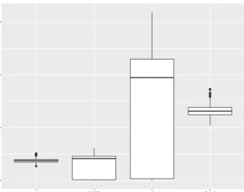
Figure 2.1 illustrates the distribution ofλs as they were obtained by the different meth-ods. As it should be expected, the mixed models approach suggested here is almost identical to the penalized quasi likelihood optimization. On the other hand, leave-one-out
cross validation produces on median λ which is high above all other approaches, while
at the same time the spread of the distribution is much wider. On the other extreme of the spectrum, principal components optimization leads to very small weights and almost no penalization. Generalized cross validation also selects small penalty weights when compared with mixed models and leave-one-out cross validation.
Method Prediction error % of ˆβ3 <0
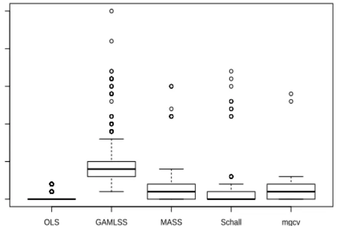
OLS 37.65 49.9 penalized 37.60 20.4 gamlss 80.71 0 MASS 37.60 19.8 Schall 37.58 0 mgcv 37.15 51.0
Table 2.1:The average prediction error of different methods.
Including a penalty termλnot only shrunks estimates towards zero, but in cases where
collinearity is present, it reduces mean squared prediction error and corrects coefficient
signs. Table 2.1 illustrates the average prediction error of all approaches. As expected the
simple linear model has the largest prediction error. Although the differences among the
models are small, using our proposed algorithm produces the smallest prediction error
with correct coefficient sign. Package mgcv gave the smallest prediction error but has 51
2.3. Simulation 13
the ordinary least squares model have an opposite sign from the real one.Multicollinearity
leads to estimates of coefficients with wrong signs (Greene, 2012). The wrong sign is
examined only for β3 because it has correlation with other two independent variables.
Table 2.1 presents in the third column the percentage of cases where ˆβ3 coefficient was
mistakenly estimated as negative. Three out of four methods estimate a correct sign for the
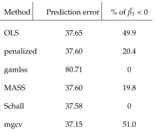
coefficient. Figure 2.2 described the computation time with respect to the methods. Schall
and MASS gave the smallest computation time.
Figure 2.2: Boxplot of computation time with respect to method for the simulated data with correlation between the independent variables
A second simulation study was also applied to investigate the performance of the meth-ods. This time, the regressors had the same distributional assumptions, however, corre-lation amongst them was 0. The data were simulated this way to investigate how each method performs when in fact penalization is not necessary. We simulated a single data
set with a sample size of 500, and generated one outcome variable y, and four covariates
x1,x2,x3,x4which
x1 ∼ N(0,1)
x2 ∼ N(0,1)
x3 ∼ N(0,1)
The covariatesx1,x2,x3,x4 are independent of each other. The response y was generated
from y = 0.7x1 − 0.3x2 + 0.2x3 +0.2 where ∼ N(0,1). The data set was then split
into a training (labelled d1) and testing data set (labelled d2), of size n1 = 400 and n2 =
100. A simple linear regression model was fitted to the training data along with four
more penalized approaches based on different methods of penalty weight optimization.
These approaches were: penalized quasi likelihood optimization using package gamlss,
generalized cross validation using packageMASS, integrated model selection via GCV using
package mgcvand optimization via random effects models suggested here using Schall’s
2.4. Summary 15
0 2 4 6
gamlss MASS Schall
Method
Lambda
Figure 2.3: Distribution of estimatedλs based on different methods of optimization for the simulated data with no correlation between the independent variables
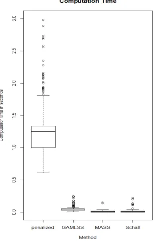
Figure 2.3 illustrates the distribution of estimated λs. The graph reveals that both
methods based on extended likelihoods (labelled as Schall and gamlss) overestimate the
importance of the penalty. The medianλweight was 4.8 in both while in the one obtained by
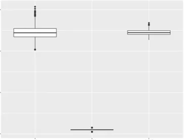
generalized cross validation, was 0.2. Figure 2.4 illustrates the distribution of computation time. The graph reveals that the computation time of ordinary least square is the shortest, following by the computation time of proposed algorithm, Schall’s algorithm.
2.4
Summary
We have introduced a method for optimizing a penalty weight in ridge-type regression problems. The method is based on mixed models algorithms although in practice one does
not need to regard the penalization as a random effect. We have shown the algorithm and
OLS GAMLSS MASS Schall mgcv 0.00 0.05 0.10 0.15 0.20 0.25 Computation Time Method
Computation time in seconds
Figure 2.4: Distribution of computation time based on different methods of optimization for the simulated data with no correlation between the independent variables
The suggested method can work in any type of regression model, regardless of the distribution assumption of the response or the link function. In this work we have shown the advantages of our approach within the context of linear regression. Perperoglou has showed in other texts how the method can be used in survival analysis (Perperoglou, 2014). In future work we aim to show how the method performs when fitting Poisson or binary data.
We presented two simulation studies. As discussed earlier, some caution is needed when applying penalized methods in data that do not require that complexity from the model. Cross validation methods were able to perform quite well in the absence of collinearity and
showed thatλhas to be near zero, i.e. they ended up with no shrinkage of the coefficients.
When mixed models methods were applied, some shrinkage was always present in the model. In any case, preliminary analysis of the data should reveal whether a penalty is needed or not.
2.4. Summary 17
It should be noted that using a mixed models approach as the one discussed here is similar to the approach within gamlss models. Both methods use a restricted maximum
likelihood approach (REML) to estimate a variance of a random effect, and use that
vari-ance to obtain the penalty weight. The only difference is that Rigby and Stasinopoulos
(2013) used their approach to optimize a roughness penalty when fitting regression splines for smoothing. An extension of either methods would be very useful in cases where a roughness penalty form smoothing models is needed in a model that also accounts for correlation, or in cases where penalties are applied into more than one dimensions. A
sim-ilar idea has been explored in the Penalized Regression with Individual Deviance Effects
models (PRIDE) (Perperoglou and Eilers, 2010). Unlike the other regression models, this
model not only involve independent variables but also include individual deviance effects.
Besides the model produces covariates estimates which give a general pattern of data, it gives information whether there is an invisible systematic pattern in data.
Chapter 3
Ridge Regression in Poisson Models and
Logistic Models
3.1
Introduction
In the previous chapters, optimized ridge regression in generalized linear models was discussed, where the response variables have a normal distribution. In generalized linear models, the response variables belong to the exponential family of distributions. The most famous members of exponential families are normal, binomial, and Poisson distributions. Here we focus on generalized linear models with binomial and Poisson responses. The binomial distribution has applied in a lot of fields. It is used when there are two possi-ble outcomes. It is applied for examining the presence of a characteristic. The Poisson distribution is often used to model rare events.
3.2. Optimized Poisson Ridge Regression and Logistic Ridge Regression 19
In Section 3.2, penalized Poisson regression will be presented followed by penalized logistic regression. In Section 3.3, we will illustrate the methods on practical applications.
3.2
Optimized Poisson Ridge Regression and Logistic Ridge
Regression
Poisson regression analysis is commonly used for modelling data with a count
indepen-dent variable. Suppose Y = (y1,y2, . . . ,yn) is an i.i.d sample from a Poisson distribution
with parameterµ, the likelihood is
L(β) = n Y i=1 µyi i e −µi yi!
and the loglikehood is
l(yi|β)= n
X
i=1
yilogµi−µi
As it has been explained in the previous chapter, the penalized log-likelihood for this model is obtained from subtracting a ridge penalty term from the log-likelihood (equation 2.2). The log-likelihood for penalized log-linear Poisson model can be written as
l∗ β = n X i=1 (yiηi−µi)− 1 2λ p X j=1 β2 j
where the link function isg(µi)=ηi =logµi =xTi β. The estimated coefficients are given by iterative weighted least square (IWLS):
ˆ
β=(X0W˜ X+λI)−1X0W˜ z˜
with the weightsW˜ is a diagonal matrix with elements a vectorµon the diagonal and the
intermediate variablez˜ =(y−µ)+µη.
As for logistic regression is commonly used for data with binomial response variable.
SupposeY+=(y+1,y+2, . . . ,y+n) is an iid sample from a binomial distribution with parameter
nandµ+, the likelihood is
L(β) = n Y i−1 µy+i i (1−µ+i)1 −y+ i
and the loglikehood is
l(β)= n X i=1 y+i η+i −log(1+eη+i )
where the link function is g(µ+i)=η+i =log
µ+ i 1−µ+ i .
Similar to Poisson ridge regression, the penalty is subtracted from the log likelihood:
l∗ β= n X i=1 y+iη+i −log(1+eη+i) − 1 2λ p X j=1 β2 j
3.3. Applications 21
where the weightsW+, a diagonal matrix with the diagonal elements:
w+ =nµ+(1−µ+)
and the intermediate variable ˜z+:
˜
z+=η++ y
+−µ+
µ+(1−µ+)
As mentioned on previous chapter, the choice of penalty weight λ is important. The
Poisson ridge regression and the logistic ridge regression will be optimized by the Schall’s algorithm. The performance of algorithm will be compared to other model selection methods such as Akaike information criterion (AIC), Bayesian information criterion (BIC) and generalized cross validation (GCV).
3.3
Applications
The performance of the proposed method is investigated on real-life data and simula-tion. First, Schall’s algorithm will be applied for a pattern of terrorism data in Afganistan between 1994-2008 (Piazza, 2012). Second, data with non-correlated covariates from Pois-son distribution and binomial distribution will be generated. The simulation is designed in such a way to produce a data set where no penalty would be required. Finally, data set with correlated covariate from Poisson distribution and binomial distribution will be generated. The performance of the Schall’s algorithm will be compared with AIC, BIC and GCV.
3.3.1
Example
A pattern of terrorism in Afganistan between 1994-2008 would be modelled. Data is published in Piazza (2012). This data set is obtained from 34 provinces. The aim of the analysis is for examining the relationship between terrorism in Afganistan and the opium trade, various economic development, infrastructure, geographic, security, and cultural
factors. The response (y) is the total terrorism incidents, and has median 22 incidents.
The predictor variables are the average annual opium cultivation (opium in hectares), area (in hectares), mountainous (in %), literacy rate (literacy in %), access to drinking water (water in %), below minimum calories(calories in %), all-season roads (roads in %), under
five mortality (mortality, out of 1000), Pashtun majority (majority, 1=Yes, 0=No), and the
mean of foreign troops (troops in yearly). Median of the average annual opium cultivation, and foreign troops are 594 hectares and 4256 soldiers. Median of percentage mountainous, literacy rate, access to drinking water, below minimum calories, and all-season roads are 40.1 %, 17.5 %, 28 %, 28 %, and 43 %. There are sixteen provinces which is Pashtun majority (47 %). In this analysis, covariates are scaled to zero mean and unit standard deviation.
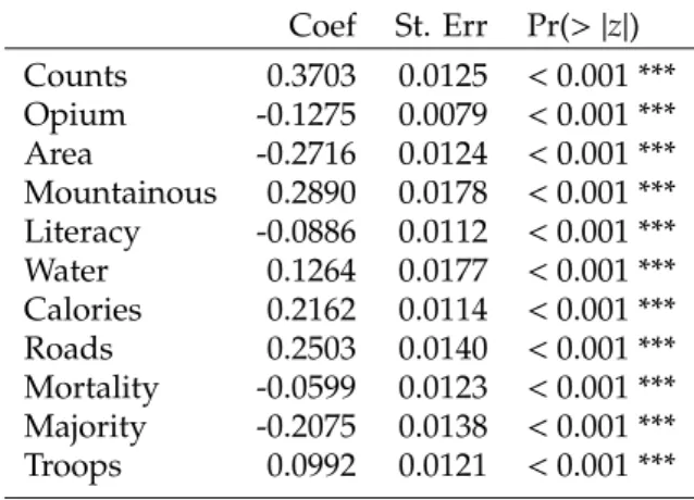
The first model applied is a simple Poisson regression. The results in Table 3.1 shows that all covariates are significant. However, these are highly correlated data. Opium has a correlation with area (0.48), mountainous has a correlation with all-season roads (-0.65) and acces to drinking water (-0.68), below minimum calories has a correlation with literacy rate (-0.46), and majority has a correlation with acces to drinking water (0.49).
3.3. Applications 23 Coef St. Err Pr(>|z|) Counts 0.3703 0.0125 <0.001 *** Opium -0.1275 0.0079 <0.001 *** Area -0.2716 0.0124 <0.001 *** Mountainous 0.2890 0.0178 <0.001 *** Literacy -0.0886 0.0112 <0.001 *** Water 0.1264 0.0177 <0.001 *** Calories 0.2162 0.0114 <0.001 *** Roads 0.2503 0.0140 <0.001 *** Mortality -0.0599 0.0123 <0.001 *** Majority -0.2075 0.0138 <0.001 *** Troops 0.0992 0.0121 <0.001 ***
Table 3.1: The simple Poisson regression results show that all covariate has a significant P-values. In column 2 and 3, coefficients and standard errors of each variables are given. The last column shows that each variable has a significant P-values (less than0.001). However, they are highly correlated data. Opium has a correlation with area (0.48), mountainous has a correlation with all-season roads (-0.65) and acces to drinking water (-0.68), below minimum calories has a correlation with literacy rate (-0.46), and majority has a correlation with acces to drinking water (0.49).
In order to get the optimal model for this data, a Poisson penalized ridge regression is used. For model selection, Akaike criterion (AIC), Bayesian criterion (BIC), generalized cross validation (GCV) and Schall’s algorithm are used.
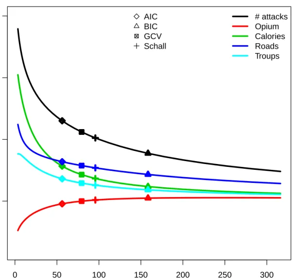
The optimal coefficients from three criterions and Schall’s algorithm can be seen in
Figure 3.1. Schall’s algorithm gives λ = 95.78. For one terrorism incident, opium, area,
mountainous, literacy, water, calories, roads, mortality, majority, and troops contribute 0.0018, 0.0023, -0.0234, 0.0510, 0.0687, 0.0367, 0.0539, -0.0440, 0.0395, and 0.0258. The best
coefficients from Schall’s algorithm are located in the middle of three other criterions.
Schall’s algorithm has a simpler algorithm than other criterions because the weight of
penaltyλis estimated and the iteration, which are done before convergence is usually less
0 50 100 150 200 250 300 0.0 0.1 0.2 0.3 λ coefficients AIC BIC GCV Schall # attacks Opium Calories Roads Troups
Figure 3.1: The coefficients of five covariates are shrunk to zero. AIC, BIC, GCV and Schall’s algorithm give different optimal fit. The optimal coefficients from Schall’s algorithm (+) (λ = 95.78) are located in the middle of three other criterions.
3.3.2
Datasets Simulations for non-correlated covariate
In this subsection, data sets with non-correlated covariate will be generated. Penalized regression will be applied on them, and some model selections will be used for choosing
3.3. Applications 25
the best model.
3.3.2.1 A non-correlated Poisson regression model
The data set with a sample size of 500 is generated. The data set has four covariates
x1,x2,x3,x4where each covariate has a standard normal distribution and are independent
of each other. The response variable is random Poisson with a parameter equal to exp Xβ
whereβ=(1,−0.4,0.7,0.2). 1000 samples are generated and analyzed.
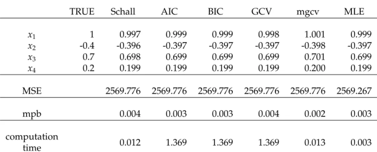
Poisson and Poisson ridge models are fitted the simulated data. According to Table 3.2,
it can be seen that there are no differences between the different methods. Therefore, for
non-correlated data, the simple Poisson regression analysis is enough.
3.3.2.2 A non-correlated logistic regression model
The data is generated data with four independent covariatex1,x2,x3,x4from a standard
normal distribution and are independent of each other. The response variable is a random
binomial with a parameter equal to exp(Xβ)/(1 +exp(Xβ)), where β = (1,−0.4,0.7,0.2).
There are 1000 samples with different sample size: 400, 450, 475, 500, and 1000.
The data set is analyzed by logistic regression and logistic ridge regression. The results are displayed in Table 3.3. It can be seen that MLE is quite better than penalized regression (The value of MSE is the smallest). According to the theory, non-correlated covariate data doesn’t need ridge regression.
TRUE Schall AIC BIC GCV mgcv MLE x1 1 0.997 0.999 0.999 0.998 1.001 0.999 x2 -0.4 -0.396 -0.397 -0.397 -0.397 -0.398 -0.397 x3 0.7 0.698 0.699 0.699 0.699 0.701 0.699 x4 0.2 0.199 0.199 0.199 0.199 0.200 0.199 MSE 2569.776 2569.776 2569.776 2569.776 2569.776 2569.267 mpb 0.004 0.003 0.003 0.004 0.002 0.003 computation time 0.012 1.369 1.369 1.369 0.013 0.003
Table 3.2: The average of coefficients of Poisson regression using ridge regression for non-correlated data. Schall’s algorithm, AIC, BIC, GCV and MLE doesn’t give different MSE and mean percentage of bias (mpb) value. So the simple Poisson regression analysis is enough.
3.3.3
Datasets Simulations for correlated covariates
In this subsection, the algorithm will be applied to the simulation. The data will be
generated with the correlation coefficients 0.90, 0.95 and 0.99. The aim of this experiment
is illustrating the performance of Schall’s algorithm for estimating the penalty weight even for highly correlated designs.
3.3.3.1 A correlated Poisson regression model
The simulation is generated for a correlated data with four random covariates. Each covariate has a correlation with other covariates with the same value of correlation, i.e. 0.90, 0.95, and 0.99. The response variable is random Poisson with a parameter equal to
exp Xβ
whereβ=(−0.309,0.7503,0.301,−0.501). Sample sizes are 20, 30, 50, and 80. 1000
samples are generated and analyzed with Poisson ridge regression. From the Table 3.4, it can be seen that MSE that resulted from Schall’s algorithm are the smallest among other criterions.
3.3. Applications 27
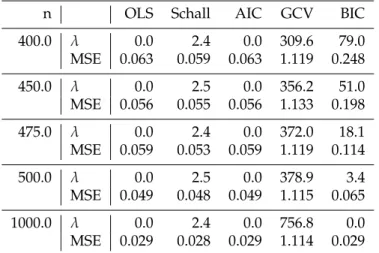
n OLS Schall AIC GCV BIC
400.0 λ 0.0 2.4 0.0 309.6 79.0 MSE 0.063 0.059 0.063 1.119 0.248 450.0 λ 0.0 2.5 0.0 356.2 51.0 MSE 0.056 0.055 0.056 1.133 0.198 475.0 λ 0.0 2.4 0.0 372.0 18.1 MSE 0.059 0.053 0.059 1.119 0.114 500.0 λ 0.0 2.5 0.0 378.9 3.4 MSE 0.049 0.048 0.049 1.115 0.065 1000.0 λ 0.0 2.4 0.0 756.8 0.0 MSE 0.029 0.028 0.029 1.114 0.029
Table 3.3:MSE from non-correlated logistic data for different sample sizes i.e. 400, 450, 475, 500 and 1000. The value of MSE for MLE is small. So the simple logistic regression analysis is enough.
OLS Schall AIC GCV
rho=0.90 20 1.539 0.770 1.361 0.959 30 0.838 0.572 0.878 0.905 50 0.465 0.364 0.549 0.765 80 0.287 0.284 0.313 0.584 rho=0.95 20 3.009 1.086 2.061 0.997 30 1.758 0.835 1.452 0.972 50 1.031 0.600 1.052 0.924 80 0.598 0.450 0.684 0.811 rho=0.99 20 18.079 1.617 7.705 1.042 30 9.960 1.598 5.506 1.126 50 5.426 1.276 3.785 1.096 80 3.290 1.069 2.521 1.113
Table 3.4: MSE from correlated count data in different correlation coefficients (0.90, 0.95, and 0.99) and different sample sizes(20, 30, 50, and 80). MSE which is resulted from Schall’s algorithm are the smallest (ρ = 0.90 and ρ=0.95). Forρ=0.99, MSE from Schall’s algorithm and GCV give similar performance.
3.3.3.2 A correlated logistic regression model
In this subsection, a correlated data will be generated with four random covariates that
have a multivariate normal distribution with meanµ=0 and constant standard deviation
to exp(Xβ)/(1+exp(Xβ)) where β = (−0.309,0.7503,0.301,−0.501). Each covariate has a
correlation with other covariate. Every correlation has the same coefficient, i.e. 0.90, 0.95,
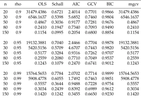
and 0.99. Sample sizes are 20, 30, 50, 80, and 150. 1000 samples are generated and analyzed with logistic ridge regression.
n rho OLS Schall AIC GCV BIC mgcv
20 0.9 31479.4386 0.6721 2.4014 0.7701 0.9866 31479.4386 30 0.9 6546.1637 0.5398 5.6852 0.7460 0.9804 6546.1637 50 0.9 0.4867 0.3036 0.9177 0.7281 0.9676 0.4867 80 0.9 0.2410 0.1947 0.7340 0.7093 0.9490 0.2410 150 0.9 0.1154 0.0995 0.2054 0.6800 0.8854 0.1154 20 0.95 19132.3881 0.7040 2.4466 0.7704 0.9878 19132.3881 30 0.95 5420.5156 0.5709 4.6707 0.7443 0.9820 5420.5156 50 0.95 0.5177 0.3284 0.9316 0.7262 0.9707 0.5177 80 0.95 0.2559 0.2080 0.7710 0.7049 0.9537 0.2559 150 0.95 0.1243 0.1079 0.2470 0.6741 0.9012 0.1243 20 0.99 15764.5653 0.7784 2.0702 0.7714 0.9899 15764.5653 30 0.99 5908.4778 0.6055 1.7492 0.7463 0.9851 5908.4778 50 0.99 0.5557 0.3644 0.9488 0.7228 0.9754 0.5557 80 0.99 0.3034 0.2439 0.8392 0.6989 0.9612 0.3034 150 0.99 0.1420 0.1242 0.3455 0.6650 0.9230 0.1420
Table 3.5: MSE from correlated binomial data in different correlation coefficients (0.90, 0.95, and 0.99) and different sample sizes(20, 30, 50, 80, and 150). MSE which is resulted from Schall’s algorithm are the smallest
Logistic ridge regression has been applied for the data sets. The selection methods: AIC, GCV, BIC, and the proposed methods, Schall’s algorithm are compared. The MSE values can be seen on Table 3.5. It can be seen that all MSE that resulted from Schall’s algorithm is the smallest among other criterions.
3.4
Summary
Penalized Poisson ridge regressions give a better result for a correlated data such as
3.4. Summary 29
with the right sign for correlated covariates. Mountainous has a different sign of coefficient
(-), as we know before, it has a negative correlation with roads and water and the value of
coefficient for roads and water are positive. Majority also has a different sign of coefficient
(+), and it has a positive correlation with water.
In order to know the performance of algorithm, MSE was calculated. MSE for penalized regression using Schall’s algorithm from correlated Poisson datasets and correlated logistic datasets are the lowest compare with MSE from other criterions.
Chapter 4
Generalized Additive Models
4.1
Introduction
The linearity assumption is violated for some applications. For example, mcycle data
set consists of 133 observations with a series of measurement of head acceleration in a simulated motorcycle accident, used to test crash helmet. Based on Figure 4.1, it is obvious that a simple linear regression is not the best model for this dataset. We try to use a polynomial regression for this. In this case, the linear regression model sometimes produce incorrect values. Transformation or higher-degree polynomials can be used , but this needs a good deal of expertise and time.
Figure 4.2 shows the polynomial regression can fit to mcycle dataset for degree five, ten, fifteen and twenty. As the degree is higher, the fit is more sensitive. It can be seen there are unexpected wiggles. Under 15 ms, the datasets give constant acceleration but the polynomial regressions is oscillatory between the data points and it also can be seen
4.1. Introduction 31
Figure 4.1: Scatterplot of the motor-cycle impact data. It can be seen that a simple linear regression is not the best model.
above 50 ms, for the polynomial regressions degree 20, the curve is not representing what happened on the data set.
Some methods have been developed for smoothing a scatterplot, for example: using a local weighting scheme (Cleveland, 1979), and the spline smoothing (Silverman, 1985; Craven and Wahba, 1978; De Boor, 1972). Generalized additive models (GAMs) give a solution for this kind of data (Hastie and Tibshirani, 1986). GAMs replace the linear combination with the respondent variable in GLMs with a sum of smooth functions of covariates. In this chapter, the definition of GAMs, penalized splines (P-splines), optimal smoothing, GAMs with P-splines and the application will be discussed.
Figure 4.2: Polynomial regressions are applied tomcycle. It can be seen that as the degree is higher, the fit is more sensitive. The polynomial regression degree 20 above 50 ms does not represent what happened on the data set.
In Section 4.2, b-splines basis function will be explained. Next, in Section 4.3, penalized splines splines) will be explained. After that, in Section 4.4, GAMs with P-splines (P-GAMs) will be discussed. In Section 4.5, the Schall algorithm for P-GAMs will be discussed. In Section 4.6, the algorithm will be applied to a datasets. Finally, Section 4.8 is the chapter summary.
4.2. B-spline basis functions 33
4.2
B-spline basis functions
There are two properties on B-spline basis functions i.e., the domain is divided by knots
and each basis function degreek,Bj,k(x) (j-th basis function degreek), are zero on the entire
interval except on a few adjacent subintervals (k+1 subintervals ork+2 knots). As a result,
B-splines basis functions are strictly local.
Suppose a set of data{x,y}, wherexis the independent variable andyis the dependent
variable with n observations. The sett = {t
1,t2, . . . ,tk+(q+1)}, called the knot vector which
tj <tj+1, is defined to obtain aqparameter B-spline basis. A B-spline degreek(orderk+1)
can be presented as:
f(x)= q
X
j=1
Bj,k(x)aj
where qis a number of parameter B-spline basis andaj are B-splines coefficients and can
be viewed as the amplitudes of B-splines. Degreek must be 1 ≤ k ≤ q+1. The shape of
the basis functions is only dependent on the knot spacing. The positions of knots and the degree can modified to change the shape of a B-spline basis curve.
Theqparameter B-spline basis functions degreek, Bj,k(x), are most easily defined
recur-sively referred to as the Cox-de Boor recursion formula (De Boor, 1972):
Bj,k(x)= x−tj tj+k−tj Bj,k−1(x)+ tj+k+1−x tj+k+1−tj+1 Bj+1,k−1(x)
where Bj,0(x)= 1 ,tj ≤x<tj+1 0 , else
Figure 4.3:Illustration of B-spline bases degree 1 with knot sequence t={0,0.2,0.4,0.6,0.8,1.0}
For example, the B-splines bases with degree 1 with knot sequencet ={0,0.2,0.4,0.6,0.8,1.0}
can be seen in Figure 4.3. One basis function consists of two linear pieces. It is defined
on two subintervals (three knots); one piece fromtj totj+1 and one piece fromtj+1 totj+2.
The knots are tj, tj+1 and tj+2. A basis function B1,1 is a non-zero function on the interval
[t1,t3]=[0,0.4]. Outside the interval [0,0.4], a basis functionB1,1is a zero function.
The B-splines bases with degree 2 with same knot sequence can be seen in Figure 4.4.
One basis function is defined on three subintervals (four knots). A basis function B1,2 is
a non-zero function on the interval [t1,t4] = [0,0.6]. Outside the interval [0,0.6], a basis
4.3. Penalized splines (P-splines) 35
Figure 4.4:Illustration of B-spline bases degree 2 with knot sequencet={0,0.2,0.4,0.6,0.8,1.0}
Taking into account the regression ofndata points (xi,yi) on the setqB-splinesBj(.). The
fit of the data can be expressed by the sum of squared errors (SSE):
S= n X j=1 yi − q X i=1 Bj(x)aj 2
aj can be estimated using an iterative method of scoring for GLM. The good fit of data is
indicated by lowS. The smoothness of the curve will depend on the number of B-splines
and the valuea. Ifajfor allas are nearly equal, next the function will be constant. Ifajvary
wildly, then the function will be unstable.
4.3
Penalized splines (P-splines)
B-splines have stable numerical properties, but the user has to decide the number and the position of knots. The number of knots influence the fit, too many knots give an overfit model and too few knots give an underfit model. Penalized B-splines (P-splines) introduce
a penalty on roughness ofawhile using a B-spline with a large number of knots (Eilers and
Marx, 1996). P-splines combine a B-spline and a difference penalty. The position of knots
usually are defined as equally spaced knots.
S∗= n X i=1 yi− q X j=1 Bj(x)aj 2 +λ q X j=k+1 (∆daj)2 (4.1)
where ∆d is the finite-order differences of the coefficients of adjacent B-splines andλ is a
penalty weight. The first order differences can be written as:
q−1 X j=1 (∆aj)2= q−1 X j=1 (aj+1−aj)2=|D1a|2 =a21−2a1a2+2a22−2a2a3+. . .+a2q
This can be written in matrix form as:
(D1) 0 D1 = −1 0 0 0. . .0 1 −1 0 0. . .0 0 1 −1 0. . .0 ... 0 0 0 0. . .1 −1 1 0 0. . .0 0 −1 1 0. . .0 0 0 −1 1. . .0 ... 0 0 0 0. . .1
The second order difference is:
4.4. Univariate Smoothing with GAMs with P-splines(P-GAMs) 37
So the second order difference operator∆2can be represented in matrix as:
D2 (q−2)×q= 1 −2 1 0. . .0 0 0 0 1 −2 1. . .0 0 0 0 0 1 −2. . .0 0 0 ... 0 0 0 0. . .1 −2 1
Thed-order difference operator∆d() (Dd) can be called out withR-codeby:
D=diff(diag(n),diff=d).
The coefficients is estimated from minimizingS∗in 4.1:
ˆ
a=(B0B+λP)−1B0y
whereBis a matrix consists of the elementsb•j =Bjk(x), the jth B-splines function andPis
the sum of squares of differences,P=D0dDd,d=0,1,2, . . ..
4.4
Univariate Smoothing with GAMs with P-splines(P-GAMs)
Hastie and Tibshirani (1986) introduced generalized additive models (GAMs) in order
to cover nonlinear covariate effects. They proposed to change a linear formXβ in a GLM
with a sum of smooth functions of the explanatory variablesP
form: g(E(y|X))= p X i=1 si(xik) (4.2)
where p is the number of covariates, xi j is k-th observation for i-th covariates. In this
chapter, the univariate smoothing will be examined. Let a GAM model containing one smooth function of one covariate,
yk =s(xk)+i (4.3)
where yk is a response variable, xk a covariate, s a smooth function and the k are i.i.d
N(0, σ2) random variables.
The functions() can be estimated by choosing a basis, defining the space of functions of
which s (or a close approximation to it) is an element. Marx and Eilers (1998) proposed
GAMs with P-splines (termed P-GAMs) which has fj = Bjkaj as the jth GAM component
whereBjk is the B-spline matrix (withqj knots) of dimensionm×qj andaj is the vector of
coefficient associated with the B-spline bases. The smoothness can be achieved from the fit
to the data which can be expressed by the sum of squared differences
S∗∗ = m X i=1 yi− q X j=1 bi jaj 2 .
4.5
Optimal Smoothing
In order to regularize the smoothness and avoid knot selection scheme, P-splines recom-mend using a large number of equally space knots (Eilers and Marx, 1996). The estimate
4.5. Optimal Smoothing 39
coefficientais obtained from an iterative technique:
ˆ at+1 =(B 0 ˆ WtB+λP) −1 B0Wˆtzˆt
until convergence, whereWˆt andzˆt are the weight matrix and adjusted dependent vector
used in GLM estimation. A difference penalty is applied for smoothing splines.
Besides the number and the degree of B-spline basis function, the smoothness of an estimated curve on generalized additive models using P-splines is influenced by the weight of penalty. The optimal weight of penalty can be obtained by some methods. Marx and Eilers (1998) proposed to use information criterion (IC) to get the optimal weight of penalty:
IC=dev(y;a, λ)+δtrace( ˆH)
where ˆH = B(B0 ˆ
WB+λP)−1
B0 ˆ
W. The estimated effective dimension ED can be obtained
from trace( ˆH). It is more efficiently computed using trace( ˆH)=trace(B0 ˆ
WB+λP)−1
.
The Schall’s algorithm will be proposed for selecting the optimal weight of penalty. It has the following steps:
1. For given ˆσ2,λˆ estimate the coefficient ˆaby:
ˆ
2. Given estimates of coefficients ˆa, variance estimators are obtained from (B0WBˆ +λP)ˆa=B0W ˆˆ z ˆ σ2 = (y−Xβˆ) 0 (y−Xβˆ) n−ED and ˆ τ2 = aˆ 0 D0 dDdaˆ ED
where ED stands for effective dimensions and is the trace of the hat matrix of the
mode (Hoaglin and Welsch, 1978). An estimate of the penalty weight ˆλcan be then
given by: ˆ λ= ED ˆ a0D0 dDdaˆ
3. Iterate until the estimated penalty weight ˆλconvergence.
4.6
Application
A data set consists of 133 observations with a series of measurement of head acceleration in a simulated motorcycle accident, used to test crash helmet. Time is measured in mil-liseconds after impact and head acceleration. In this section, mcycle data set will be used. It is used by Silverman (1985) for giving understanding about the spline smoothing. The data set is obtained from Schmidt et al. (1981).
4.6. Application 41
Figure 4.5: B-spline regressions with different number of knots. Upper left, the fit is resulted from B-splines with 20 knots. Upper right, the fit is resulted from B-splines with 25 knots. Lower left, the fit is resulted from B-splines with 30 knots. Lower right, the fit is resulted from B-splines with 30 knots. As bigger the number of knots, the fit is more wavy
An alternative method to solve this problem is B-spline basis regression. Regression fit for cubic spline with 20, 25, 30, and 40 equally-sized segment can be seen in Figure 4.5. It can be seen that for more knots, the curve is more wavy.
In order to solve the problem in choosing the number of knots, P-GAMs with P-spline is applied and the optimal smoothing used Schall’s algorithm. The result with 40 knots can be seen in Figure4.6. The curve which is resulted from P-spline is more smooth than the curve which is resulted from B-spline.
Figure 4.6: The curve is resulted from P-spline with 40 knots. The optimal weight of penalty of P-spline regression is selected automatically using Schall’s algorithm.
4.7
Simulation
Schall’s algorithm will be applied for smoothing a simulated data set. The data set
consists of 200 observations. The predictor has a standard normal distribution (N(0,1))
and the response variabel isy=b0+b1∗sin(2∗x)3+e2where (b0,b1)=(5,10) andeis an error
with a normal distributionN(0,h(x)). h(x) is a function which performs heteroscedasticity
function:
h(x)=1+0.1x.
4.7. Simulation 43 −2 −1 0 1 2 −5 0 5 10 15 20 simulated data x y
Figure 4.7: Scatterplot of the simulated data. It can be seen that a simple linear regression is not the best model.
Figure 4.8: Left: the smoothing result from optimized P-GAM.;Right: the smoothing result from tensor product (package mgcv).
P-GAM using Schall’s algorithm as automatic optimization will be applied and the result will be compared with smoothing using tensor product. The result is quite similar using the same number of knots (40 knots). Computation time of P-GAM using Schall’s algorithm (0.20 second)is shorter than Computation time of tensor product smoothing (0.86 seconds).
4.8
Summary
Generalized Additive Models can be presented with generalized linear models. In order to get GLMs form, smooth functions in GAMs are replaced by P-splines. If in GLMs, there is linear combination of covariates then in GAMs with P-splines (P-GAMs), there is the linear combination of basis functions.
P-GAMs have some advantages such as GAM estimation is reduced to (generalized) linear regression with a manageable penalty; the system of equations is a low dimension and easy to solve; all the smooths are estimated simultaneously; the resulting GAM fit is compactly summarized by relatively few numbers of parameters that facilitate future prediction and standard errors, and regression diagnostics can be computed with relative ease (Marx and Eilers, 1998).
The weight of penalty choosing is the important steps in penalized regression. The Schall’s algorithm is applied for choosing the optimal weight of penalty. This algorithm uses iterative to find the best model. It usually only needs a few number of iteration.
Chapter 5
Lasso Regression
5.1
Introduction
The lasso is a commonly used method for a variable selection. The method uses L1
penalization to shrink estimates. It is often used on high dimensional data, not only to solve high dimensionality problem but also as a variable selection methods.
In this chapter we will propose a method for optimising a penalty weight. The novelty
of our approach has to do with re-writing the lassoL1penalty as anL2type ridge penalty.
Having done that, we will be able to optimise the weight using similar approaches to those of previous chapters. The procedure is a combination of a ridge regression approximation (Tibshirani, 1996), and a sum of absolute values approximation (Schnabel and Eilers, 2013). The algorithm will be applied to prostate data and simulation data.
The chapter is organized as follows: In section 5.2, the definition of the lasso regression will be explained. Later, section 5.3 will describe the commonly used computation for the
lasso regression. The proposed algorithm will be described in Section 5.4. Next, Section will apply the algorithm for some data set, real and simulation. Finally, Section 5.6 give a summary for this chapter.
5.2
Definition
The lasso (Least Absolute Shrinkage and Selection Operator) is a regularized regression
method with anL1-norm penalty. It was proposed by Tibshirani (1996). Where the ridge
regression uses the sum of squared coefficients as a penalty, the lasso uses the sum of the
absolute value of coefficients, such that:
`∗ β = n X i=1 `i β−λ p X j=1 |βj|
The lasso coefficient estimatesβˆcan be presented as
ˆ β=argmax n X 1 `i β−λ p X j=1 |βj| (5.1)
or, alternatively, in matrix notation:
ˆ
β=argmax{`(β)−λkβk1}
The constraint shrinks coefficients and produces some coefficients that are exactly zero.
That means that lasso also performs variable selection, not only shrinkage. Asλincreases,
5.3. Computation 47
5.3
Computation
Tibshirani (1996) used a quadratic programming for estimating lasso coefficients.
Equa-tion 5.1 is expressed as a least squares problem with 2pinequality constraints, corresponding
to the 2pdifferent possible signs for theβjs. Although 2pmay be very large, the problem can
be solved with inequality constraints sequentially and trying to find a solution satisfying the Kuhn-Tucker conditions. The Kuhn-Tucker conditions for the lasso problem:
XT(y−Xβˆ)=λs, (5.2) where si ∈ {sign( ˆβ i)} if ˆβi ,0. [−1,1] if ˆβ i =0. ,fori=1, . . . ,p. (5.3) ˆ
β is a solution in Equation 5.1 if and only if ˆβ satiesfies Equation 5.2 and Equation 5.3 for
somes. Computation for lasso solutions with this procedure is however, expensive. The
optimal weight of the penalty can be selected by generalized cross-validation. In the next section, we will propose an alternative algorithm.
TheRpackagepenalizedimplemented a method introduced by Goeman (2010). The
al-gorithm improves the gradient-based alal-gorithm by combining gradient ascent optimization and the Newton-Raphson algorithm in order to avoid the tendency to slow convergence. The package can be used for linear regression, logistic and Poisson regression as well as the
Cox proportional hazards model. The optimal value of the tuning parameterλis chosen
Next, the R package glmnet is developed by Friedman et al. (2009). The algorithm applies cyclical coordinate descent in a pathwise fashion. The idea of pathwise coordinate
optimization is solving a sequence of single-parameter problems (βj) with a fixed value
penaltyλand holding the other parameters fixed at their current values. Equation 5.1 can
be written as: f( ˜β)= 1 2 n X i=1 yi− X k,j xikβ˜k −xi jβ˜j 2 +λX k,j |β˜k|+λ|β˜j|
where all the values ofβk fork, jare held fixed at values ˜βk(λ). The solution is:
˜ βj(λ)←S ˜ βj(λ)+ n X i=1 xi j yi−y˜i, λ (5.4)
HereS(t, λ) =sign(t)(t− |λ|)+. Iteration of 5.4 is r