Stability analysis of constrained inventory systems with transportation delay
Xun Wang a,*, Stephen M. Disney b, Jing Wang aa School of Economics and Management, BeiHang University, Beijing, 100191, China
bLogistic Systems Dynamics Group, Cardiff Business School, Cardiff University, Aberconway Building, Colum Drive, Cardiff, CF10 3EU,UK Abstract
Stability is a fundamental design property of inventory systems. However, the often exploited linearity assumptions in the current literature create a major gap between theory and practice. In this paper the stability of a constrained production and inventory system with a Forbidden Returns constraint (that is, a non-negative order rate) is studied via a piecewise linear model, an eigenvalue analysis and a simulation investigation. The APVIOBPCS (Automatic Pipeline, Variable Inventory and Order Based Production Control System) and EPVIOBPCS (Estimated Pipeline, Variable Inventory and Order Based Production Control System) replenishment policies are adopted. Surprisingly, all kinds of non-linear dynamical behaviours of systems can be observed in these simple models. Exact expressions of the asymptotic stability boundaries and Lyapunovian stability boundaries are derived when actual and perceived transportation lead-time is 1 and 2 periods long respectively. Asymptotically stable regions in the non-linear Forbidden Return systems are identical to the stable regions in its unconstrained counterpart. However, regions of bounded fluctuations that continue forever, including both periodicity and chaos, exist in the parametrical plane outside the asymptotically stable region. Simulation shows a complex and delicate structure in these regions. The results suggest that accurate lead-time information is essential to eliminate inventory drift and instability and that ordering policies have to be designed properly in accordance with the actual lead-time to avoid these fluctuations and divergence.
Keywords: Inventory; logistics; system dynamics; complexity theory
1. The introduction and motivation
One of the main objectives when designing an inventory system is to maintain its stability and robustness in the face of exterior disturbances. Since the introduction of control theory and system dynamics approaches to the field of inventory control (Simon, 1952; Forrester, 1961), many works have studied this problem. However, the significance of results obtained are frequently limited by both the uncertainty and complexity of the system structure. Often omitted factors in inventory system design include saturation (logistics constraints) and mis-specified delays (lead-times). In previous supply chain stability studies (Riddalls and Bennett, 2002; Nagatani and Helbing, 2004; Warburton et al., 2004; Disney, 2008), linear inventory system models are usually adopted. Linearity assumptions include infinite capacity, ignoring inventory limitations and return restrictions. This has greatly limited the applicability of published results, and has failed to explain many business phenomena (Riddalls et al., 2000). For instance, to maintain linearity of the commonly investigated IOBPCS (Inventory and Order Based Production Control System) models, order rates are permitted to take negative values. This means that all participants in a supply chain are allowed to return excess product freely. Specifically, a negative order rate value leads to a decrease in the inventory level at the consuming echelon and an immediate increase in the inventory level at the supplying echelon. Practically this may mean that the excess inventory is not moved from one location to another but instead will be considered to be in the possession of the upstream member until being used as part of a future replenishment (Hosoda and Disney, 2009). This assumption may be difficult to realize in reality.
Non-linear effects also play an important role in inventory systems, sometimes even a dominant role (Nagatani and
Helbing, 2004). When linearity assumptions are removed complex dynamic behaviours are present. They may even be chaotic or super-chaotic. Mosekilde and Larsen (1988) found that the operating cost of a constrained system could be 500 times higher than its linear counterpart. Larsen et al. (1999) further demonstrated this fact. Through their simulation experiments, Thomson et al. (1992) concluded that economic and business systems scarcely operate nearby their steady state. More recently, Wang et al. (2005) used the Lyapunov Exponent to identify whether an inventory system is in a chaotic state. Wu and Zhang (2007) found that the attractors of an inventory system model move with the assumed initial states, rendering it impossible to provide guidelines to avoid chaos by bifurcation analysis. Hwarng and Xie (2008) investigated several system factors that affect chaotic behaviour and discovered a
‘chaos-amplification’ phenomenon between supply chain echelons. Liu (2005) and Rodrigues and Boukas (2006) analyzed
the stability of supply chain inventory systems with piecewise linear techniques. Laugessen and Mosekilde (2006) and
Mosekilde and Laugessen (2007) studied the border-collision behaviour in piecewise linear supply chain systems. Mathematical properties of such systems, such as local and global stability conditions and bifurcations, are “very hard
* Corresponding author. Tel.: +86 10 8233 8930.
E-mail addresses: [email protected] (X. Wang), [email protected] (S.M. Disney), [email protected] (J. Wang)
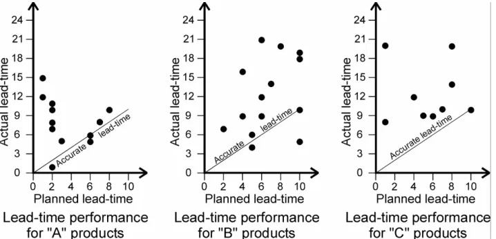
Fig. 1: Lead-time performance in an industrial setting, Coleman (1994). to investigate” and “notoriously challenging” (Sun, 2010).
In an ideal situation, production lead-time would not vary and supply chain participants would have perfect knowledge
of lead-times (Cheema, 1994). However we should not necessarily assume this is so. Time varying and misperceived
lead-times are commonly observed in industry (Fig. 1, adopted from Coleman, 1994). In particular, varying lead-time increases supply chain cost (Chaharsooghi and Heydari, 2010), exacerbates the bullwhip effect (Kim et al., 2006) and significantly affects policy making (Rossi et al., 2010). Misperceived lead-time creates a so-called phenomenon of ‘inventory drift’ and attenuates the efficacy of meeting safety stock requirements (Disney and Towill, 2005).
From this perspective, the main concern of this paper is to investigate the effect of lead-time on constrained supply chain stability, or, more specifically, a supply chain replenishment policy with Forbidden Returns. This paper is organised as follows: Section 2 models the constrained one echelon supply chain system piecewise-linearly and conducts an eigenvalue analysis; Section 3 investigates the stability of the inventory system with perfect lead-time information under unit lead-time; Section 4 focuses on the effect of lead-time change and lead-time misperception on system stability; Section 5 concludes.
2. Model of constrained supply chain systems
This paper adopts the APVIOBPCS ordering policy. A brief review of this policy will now be provided. Towill (1982)
presented a model named Inventory and Order Based Production Control System (IOBPCS) in the form of a continuous time, Laplace Transform block diagram. Edghill and Towill (1989) introduced a variable inventory target to the basic IOBPCS model, creating the VIOBPCS (Variable Inventory and Order Based Production Control System) model. John et al. (1994) proposed an Automatic Pipeline, Inventory and Order Based Production Control System, or APIOBPCS by adding work-in-process (pipeline inventory or supply line) information feedback into the production target decision process. This model has been frequently adopted and researched for its many distinguished advantages (Disney and Towill, 2003). Further, by combining VIOBPCS and APIOBPCS, a more general model, Automatic Pipeline, Variable Inventory and Order Based Production Control System (APVIOBPCS), will be derived. The full IOBPCS family is comprehensively reviewed by Sarimveis et al. (2008).
We study the discrete time APVIOPBCS replenishment policy. This policy has been frequently adopted and researched as it is of a very general nature. The popular order-up-to (OUT) policy is a special case of this APVIOBPCS model,
Dejonckheere et al. (2003). We refer interested readers to Disney et al. (2003) for more information on the
APVIOBPCS model, but we also give a definition here. When Tp= 1, the difference equations for the APVIOBPCS
inventory system are given by (1) to (6)
Forecasting 1 1 1 1 a t t t a a T
AVCON CONS AVCON
T T
Inventory AINVt AINVt1COMRATEtCONSt, (2)
Work-in-process WIP WIPt t1ORATEt1COMRATEt, (3)
Transportation delay TRANSt ORATEt1, (4)
Completions COMRATEt TRANSt1, (5)
Ordering decision
Inventory Discrepancy WIP Discrepancy (1 ) t t S t t SL t t S SL t S t SL t ORATE AVCON AVCON AINV AVCON WIP AVCON AINV WIP . (6)Equation (1) details AVCONt, an estimate of the AVerage CONsumtpion, used a forecast of future demand. The subscript t is used to index time. This forecast can be generated using any forecasting method, but here we use the exponential smoothing forecast method. Ta is the average age of the data in the exponential smoothing forecast and is linked to the so-called smoothing constant, , often used in the literature via Ta
1 1. (2) gives the inventory balance equation, where the new realisation of the Actual INVentory, AINVt is the sum of the previous actual inventory level, AINVt1 plus COMRATEt, the COMpletions from the production facilities or (deliveries from the suppliers), minus the current demand or CONSumption, CONSt. (3) is the equivalent Work In Progress (WIP) balance equation, where ORATEt1 is the Order RATE at time t1. TRANSt in (4) is an assistant variable used to describe the transportation delay in matrix form. In (5) COMRATE is the COMpletion RATE. (6) describes the production / distribution / replenishment Order RATE decision. It is made up of a single feed-forward loop based on the forecast, AVCONt and two feedback loops, AINVt and WIPt. We also have two additional controllable feedback parameters, S, SL, that are used to regulate how the feedback on the inventory levels, S
AVCONt AINVt
, and the WIP levels SL
AVCONtWIPt
is incorporated into the production ordering decision. Forbidden Returns (non-negative orders) are enforced with the maximum operator, [x]+ = max(0,x), in (6). Since there is no non-negative constraint on actual inventory, the following underlying assumptions of this model are necessary: outsourcing is available (downstream demand can still be fulfilled even if supplier’s inventory is insufficient); and shortage backorder is allowed (negative inventory can be accumulated into the next period). The above difference equations can be used to develop a dynamic simulation of the policy in software such as Excel, or more efficiently MATLAB, where evolution of each variable can be calculated iteratively. They are also easily converted into matrices that describe the system of equations: 1 0 0 0 0 1 (1 ) 1 0 0 1 0 1 0 1 0 1 1 0 1 0 0 0 a a a S SL SL S SL SL S a T T T T A , 1 1 1 1 1 1 0 0 a S SL S a T T b , 2 0 0 0 0 1 0 0 0 0 0 0 0 1 0 1 0 1 0 1 1 0 1 0 0 0 a a T T A , 2 1 1 0 1 0 0 a T b The piecewise affine model for this system is given by 1 1 1 1 1 2 1 2 1 2 , , t t t t t t t CONS S CONS S A x b x x A x b x (7)
where S1 { |x ORATE0} and S2 { |x ORATE0} are both non-degenerate polyhedral partitions of the state
space. That is, each region Si is a (convex) polyhedron with a non-empty interior. The (n–1) dimensional hyper-plane
ORATE = 0 is the boundary of the partitions.S1S2 n,
1 2 1 2
SS S S . S° is the interior of S and n is the
dimension of x. It should be noted that the boundaries are continuous, i.e., A x1 t A x2 twhenxtS1S2. Common
concepts, such as region and boundary, will be used in either the phase space or the parametrical space.
This model can be further simplified. When Tp = 1, the work-in-process is a flow rate rather than a stock level, i.e.,
TRANSt = WIPt. Moreover, since the forecasts are solely a feed-forward loop in the system, they do not affect system
stability. This allows us to decrease the dimension of the inventory system model. If we let Ta = 0, indicating that the
demand forecast is, at all times, equal to the last observed demand we can express the inventory system in three dimensions with the following matrices:
1 0 1 1 1 0 0 SL S S A , 1 1 2 1 0 S SL b , 2 0 0 0 0 1 1 1 0 0 A , 2 0 1 0 b , ORATE AINV WIP x .
Further noticing that A1 and A2 are both linear dependent, the dimension of the system can be further reduced.
Denoting the sum of on-hand inventory and work-in-process as the inventory position, that is IPt = AINVt + WIPt, we
have 1 1 1 SL S A , 1 1 2 1 S SL b , 2 0 0 1 1 A , 2 0 1 b , ORATE IP x (8)
In the following sections, we will show that stability and periodicity of the inventory system described by Eq. (1~6)
are determined by the two-dimensional dynamical system expressed in (7) and (8), and more specifically, by the
eigenvalues for A1, A2 andA1A2. These eigenvalues are:
1 2 2 1 (1 ) 4 1 (1 ) 4 , 2 2 SL SL S SL SL S A λ (9)
2 0,1 A λ (10) 1 2 (0,1 S) A A λ (11) Notice A1 has two eigenvalues and A1A2 has one eigenvalue associated with the feedback loops which need to be investigated. The eigenvalues of these matrices yield regions in the parametrical plane {SL, S} in which theinventory system behaves differently and these will now be derived and investigated.
3. Stability of the constrained APVIOBPCS model
The stability of linear systems is much easier to investigate compared to non-linear systems. There are only two patterns of dynamic behaviours which are physically possible from a stability perspective. The system could be stable, which means the trajectory will eventually return to an equilibrium point (node), no matter where it is started (insensitivity to initial value). It could also be unstable, which means the trajectory will escape to infinity. There is also a third pattern, appearing when the system is on the very edge of stability boundary called critical stability. The system will oscillate at a regular interval. However, since the boundary has a measure of zero in the parametrical space, critical stability is only available mathematically, and is not present in physical systems. Whether it exists in a supply chain system that is driven by a computer algorithm (i.e. mathematically) is a matter for debate.
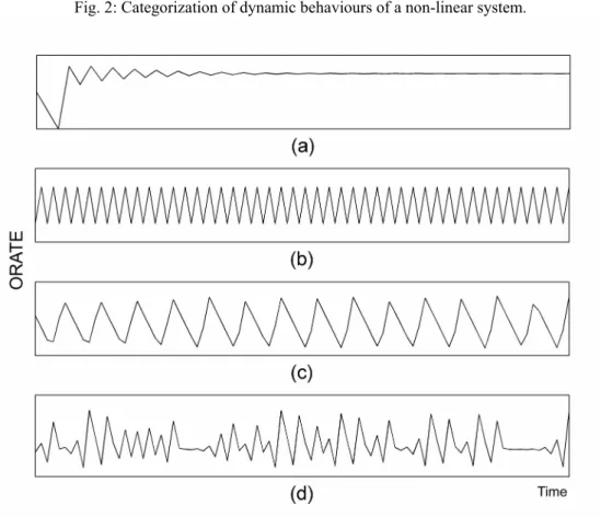
In non-linear systems however, the range of dynamic behaviours the system could exhibit is much larger. First, there could be a saddle point. A saddle point attracts trajectories from some directions and repels trajectories from other directions. Second, there are other types of attractors such as “limit cycles” and “strange attractors” that may be present. Trajectories of non-linear systems could be either convergent or divergent and can even oscillate in a bounded fashion. It could oscillate in a regular repeating pattern or in a seemingly random one. The dynamic behaviour of the system could also be highly sensitive to initial values. Dynamic behaviours of the inventory levels in non-linear systems are categorized in Fig. 2. Here we have also ranked the different dynamic behaviours from an intuitive supply chain cost viewpoint. Detailed investigations on the stability of the constrained supply chain will now be conducted.
Fig. 3 shows typical bounded dynamic patterns in the time domain.
Fig. 2: Categorization of dynamic behaviours of a non-linear system.
Fig. 3: Four typical dynamic order rate patterns (for the step response) generated by the constrained inventory system. (a) asymptotic stable; (b) periodic; (c) quasi-periodic; (d) chaotic
3.1 Lyapunovian stability and divergence
If all solutions of a dynamical system that start out near an equilibrium point xe, stay near xe forever, then the system is
Lyapunovian stable. Note that, even when the system fluctuates but never approaches the equilibrium, as long as the fluctuation is bounded, the system is Lyapunovian stable. Lyapunovian instability indicates an unbounded oscillation and a trajectory that tends to infinity. That is, it diverges.
There are two factors in the inventory system with non-negative order rates that cause divergence. One is the matrix coefficient (A1) which creates an exponential (multiplicative) monotonic divergence. The other is the affine term (b2) which creates a linear (additive) divergence. Sometimes these two factors may combine and lead to an exponential and
oscillating divergence (the characterisation of which is beyond the scope of this paper). The criteria for exponential monotonic divergence is im(λA1) 0 andλA1 1, where im(z) is the imaginary part of the complex number z. These
relations give the Lyapunovian stability regions. In linear systems, if the eigenvalues of system matrices are complex and the absolute value of eigenvalues are bigger than 1, the system will oscillate with exponential divergence. However, in piecewise linear Forbidden Returns systems, such trajectories will eventually hit the boundary. In other words, the boundary constrains or limits such trajectories from divergence. Thus the exponential divergence is always monotonic and away from the boundary.
We can derive the parametrical boundaries that separate exponential divergence from bounded responses. For Tp = 1,
when A1 has two real eigenvalues greater than 1, exponential divergence can be observed. Thus, the Lyapunovian
stability boundary for Tp = 1 is given by
S = (SL + 1)2 / 4. (12) 3.2 Asymptotic stability
If xe is Lyapunovian stable and all solutions that start near xe converge to xe, then more strongly, xe is asymptotically
stable. This means that the trajectory approaches an equilibrium point over time (Fig. 3a). This concept has similar meaning with stability in a classical linear control theory sense. In the asymptotically stable region, the system will eventually return to equilibrium. The condition for asymptotic stability isabs(λA1) 1 . When Tp = 1 this amounts to
0 < S < 2SL – 2, 0 < SL < 1 (13)
and
SL + 1 < S < 2SL – 2, 1 < SL < 3. (14) 3.3 Periodicity
Periodicityof a system is a point which the system returns to after a certain number of function iterations or a certain amount of time (Fig. 3b). Periodic behavior is defined as recurring at regular intervals, such as “every 24 hours”, or “every 4 weeks”. In this piecewise linear discrete system, boundaries of periodic movements can be obtained by studying the asymptotic stability of the corresponding matrix representing the periodic pattern. That is to say, if period
1 2 m n
S S is discovered under certain parameter settings, where m n, and power is used to express the trajectory staying in one region, then the matrix A A1m 2n is asymptotically stable. We notice that the value of n does not affect
eigenvalues of matrix A A1m 2n as long as n > 0 since the two dimensional A2 (Eq. 8) is idempotent.
For instance, conditions of periodic movement S S1 2n in T
p = 1 system can be derived by solving
1 2
abs(λA An) 1 , which
leads to 0 < S < 2. Likewise, the boundary for periodicity of S S12 2n can be obtained fromabs( 2 n) 1
1 2
A A
λ , i.e.,
2 1 1
S SL S
, where we can obtain
2 SL and 2 2 S SL . (15)
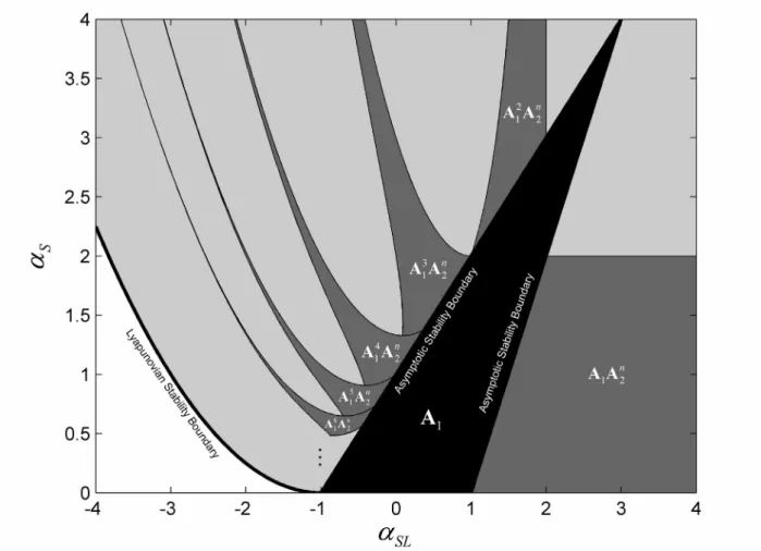
Fig. 4 shows Lyapunovian stable (white), asymptotically stable (black) and periodic (dark grey) regions for the inventory system when Tp = 1. The matrices used to derive the boundaries are also labeled. Notice that there is an
infinite number of such dark grey branches above the asymptotic stability boundary.
3.4 Quasi-periodicity and chaos
Quasi-periodicity is the property of a system that displays irregular periodicity. Quasi-periodic behaviour is a pattern of recurrence with a component of unpredictability that does not lead itself to precise measurement (Fig. 3c). Quasi-periodicmotion is, in rough terms, the type of motion executed by a dynamical system containing a finite number (two or more) of incommensurable frequencies. Values of quasi-periodic points are dense everywhere.
Mathematically, chaos refers to a very specific kind of unpredictability: deterministic behaviour that is very sensitive to its initial conditions.In other words, infinitesimal variations in initial conditions for a chaotic dynamic system lead
When chaotic dynamics occurs, the system moves in a region of phase space that is densely filled with unstable periodic orbits. The trajectory is attracted and repelled in different directions by these orbits, and the result is an irregular behaviour that is sensitive to small perturbations and parameter changes (Mosekilde and Laugessen. 2007). Quasi-periodicity and chaotic motion are both characterized by the fact that, although bounded in phase space (Lyapunovian stable), the trajectory never precisely repeats itself. This research shows that, compared to the
four-echelon beer-game model studied in Mosekilde and Laugessen (2007), such complex behaviours can be found even in
this simple model of a constrained inventory system. When the system behaves quasi-periodically or chaotically,
1
A has two complex eigenvalues outside the unit circle, and no stable periodic movement can be found. In Fig. 4,
Quasi-periodicity and chaos are represented by light grey.
Fig. 4. Stability diagram of the Forbidden Returns inventory system when Tp = 1.
To summarise the aforementioned boundaries divide the parametrical plane into several regions in which the inventory system behaves differently: asymptotically stable, periodic, quasi-periodic, chaotic and divergent. As intuition would dictate, a positive inventory feedback parameter is essential to maintain stability of the system. Furthermore, when the absolute value of SL is small, the system will be asymptotically stable. This region is limited and shaped as the black
triangle. Luckily the Order-Up-To policy (S = 1, SL = 1) lies within this region. When SL is negative, exponential
divergence can be observed. Regular periodicity can be discovered when S is small and SL is positively large. Other
areas are filled by periodical branches, quasi-periodic and chaotic parameter settings. What we can infer from the above analysis is that high S and SL values lead to chaos.
4. Stability analysis on the effect of lead-times
In this section we will analyze the effect of lead-time change and lead-time misperception on supply chain stability. We focus on actual lead-time change in the first subsection and lead-time misperception in the second. For the sake of simplicity, in these two subsections, we restrain ourselves to cases where both actual time and perceived lead-time are either one or two lead-times of the length of the ordering cycle, that is,
T Tp, p
{1, 2}. In the last subsection, we investigate how the lead-time affects the size of asymptotically stable region and Lyapunovian stability boundaries.Methods to determine stability boundaries which are proposed in the previous section are particularly useful in conducting this part of analysis.
4.1 Actual lead-time changes with perfect knowledge
For Tp = 2, using the same techniques as in the previous section, it is easy to derive stability and periodicity conditions.
For the sake of brevity we omit the predictable modeling and analysis procedures. The Lyapunovian stability boundary is given by
3 2
4SL12SL15SL 4 27S 0, (16) and its asymptotic stability conditions are:
2 2 2(1 2 ) 0 1 3 2 5 SL SL S SL SL SL for -0.5 < SL < 1; (17) 2 2 2(1 2 ) 2 1 3 2 5 SL SL S SL SL SL for 1 < SL < 2.5. (18)
If we draw boundaries of Tp = 1 and Tp = 2 together as shown in Fig. 5, we are able to visualise the different dynamic
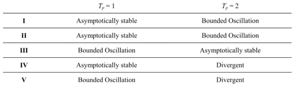
behaviours that exist when the lead-time increases from 1 to 2 and we know of this fact. Table 1 summarizes the
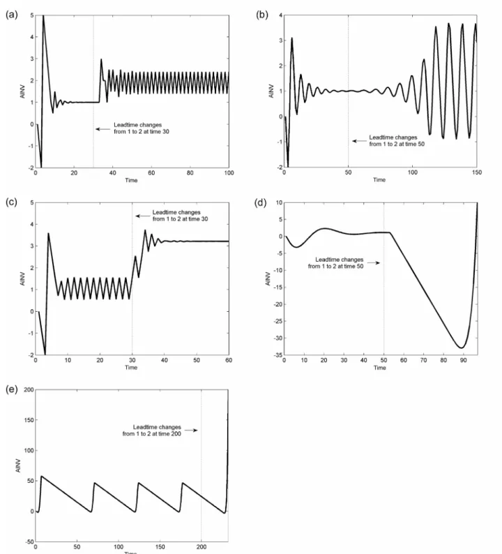
dynamic behaviour under each lead-time value, and highlights the regions where a structurally different behaviour can be observed. Since the periodic boundaries are fractal as was discovered in the previous section, we decided not to distinguish periodic, quasi-periodic and chaotic movements hereafter but identify them aggregately as ‘bounded oscillation’. Although we have assumed the lead-time can be accurately measured and the replenishment policy can be correctly updated with this lead-time information, a sudden increase of lead-time could still jeopardize system stability. That is, a system could be asymptotically stable with one lead-time but with a higher lead-time it could exhibit bounded oscillation (region I and II in Fig. 5) or even divergent behaviour (IV). In region III, a lead-time increase will actually stabilize the system. Highly volatile lead-times will increase the difficulty of maintaining system stability. Consider the following example: the decision maker ignores WIP feedback and uses 80% of inventory feedback in ordering decision (S = 0.8, SL = 0, IOBPCS system). The system is asymptotically stable under unit lead-time.
However a limited vibrating dynamic behaviour will be observed when lead-time is 2 (Fig. 6b). Fig. 5 and Table 1 are verified via simulation as shown in Fig. 6, where the system is driven by a unit step demand process, and a dotted line represents the time when lead-time changes. The length of the MATLAB simulation and the timing of the lead-time changes have been adjusted to allow the figures to be presented clearly.
4.2 Unobserved lead-time changes
In this section, the effect of lead-time on system stability in the Estimated Pipeline Variable Inventory and Order
Based Production Control System (EPVIOBPCS) will be analyzed. This policy was introduced in Disney and Towill
(2005) to eliminate a phenomenon known as inventory drift (when the system falls into a steady state with a permanent difference between the target and actual inventory levels), by calculating work-in-process level using perceived lead-time as
1 1 p 1
t t t t T
WIP WIP ORATE ORATE (19) or, after z-transform,
1 1 p T WIP z ORATE z . (20)
where Tp is the perceived lead-time. When Tp Tp the EPVIOBPCS produces the same dynamic response as the
APVIOBPCS. However, when the perceived lead-time is incorrect, i.e., Tp Tp, this method generates artificial WIP
values that are matched to the DWIP target levels and this allows the inventory to return to target levels. It is already known that when work-in-process is calculated in the conventional way (via Eq. 5), the value of Tp does not affect the
Fig. 5: Stability comparison between Tp = 1 and Tp = 2.
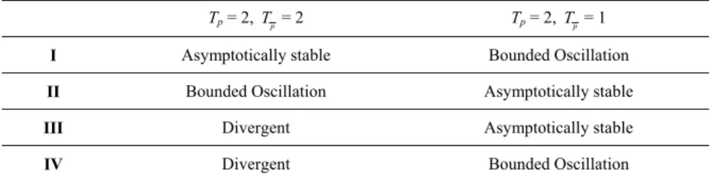
Table 1: Change of dynamic behaviour in each region with known Tp changes observed in Fig. 5. Tp = 1 Tp = 2
I Asymptotically stable Bounded Oscillation
II Asymptotically stable Bounded Oscillation
III Bounded Oscillation Asymptotically stable
IV Asymptotically stable Divergent
V Bounded Oscillation Divergent
when work-in-process is calculated based on the perceived lead-time, Tp, (with Eq. 19), then Tp changes the
dimension of the inventory system and thus it has a dramatic effect on stability and the dynamic behaviour. The characteristic polynomial for EPVIOBPCS, in the z-domain, i
s 1 ( 1) 0 p p p p T T T T SL SL S z z z for p p T T 1 ( 1) 0 p p p p T T T T SL S SL z z z for p p T T (21) When perceived lead-time is correct (Tp Tp), this polynomial becomes
1 ( 1) 0 p p T T SL SL S z z (22)
Fig. 6: Dynamic responses of Forbidden Returns APVIOBPCS with a sudden increase of lead-time under multiple parameter settings (verification of Fig. 5 and Table 1). (a) Region I: αS = 2.5, αSL = 2; (b) Region
II: αS = 0.8, αSL = 0; (c) Region III: αS = 1.8, αSL = 2; (d) Region IV: αS = 0.05, αSL = –0.8; (e) Region V: αS
= 2, αSL = –2
which characterises the APVIOBPCS replenishment policy. To maintain asymptotic stability of the system, (complex) solutions must lie within the unit circle on the complex plane. For Lyapunovian stability, at least one solution must be real and larger than one. The longer lead-time between the actual and the perceived ones determines the order of the polynomial. For specific lead-time combinations it is possible to derive the criteria analytically with the Inners approach of Jury (1974). For the general case unspecified lead-time combinations, we do not know of a solution. Let’s examine the following cases: Case (1-2), an overestimation of the actual lead-time; Case (2-1), an under
estimation of the actual lead-time. Note that we are using two hyphenated numbers in brackets to represent lead-time mis-specification scenarios, the first number representing the actual lead-time, Tp, and the second one perceived
lead-time,Tp. Parametrical boundaries for the above two cases can be derived. For the (1-2) case, the asymptotic stability region is:
2
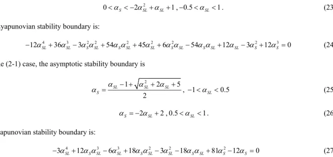
0S 2SLSL1, 0.5 SL 1. (23) The Lyapunovian stability boundary is:
4 3 2 2 2 2 2 2 3
12SL 36SL 3 S SL 54 S SL 45SL 6 S SL 54 S SL 12SL 3S 12S 0
(24)
For the (2-1) case, the asymptotic stability boundary is
2 1 2 5 2 SL SL SL S , 1 SL 0.5 (25) 2 2 S SL , 0.5SL1. (26) Its Lyapunovian stability boundary is:
4 3 3 2 2 2
3SL 12 S SL 6SL 18 S SL 3SL 18 S SL 81S 12S 0
(27)
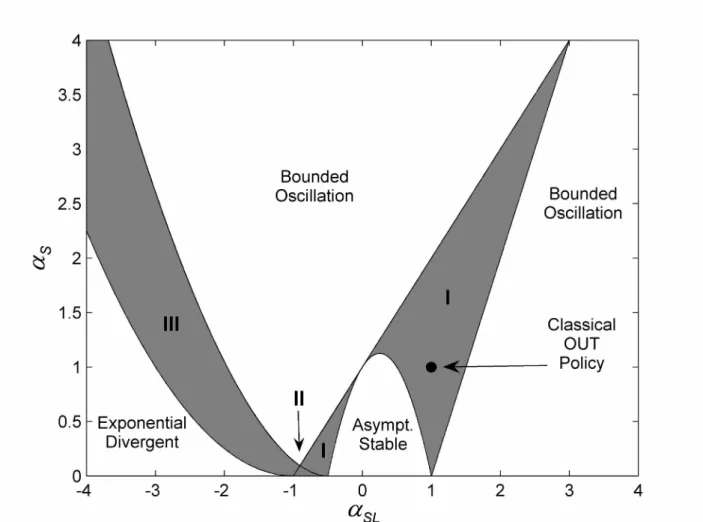
Similar to the analysis in the previous section, we obtain structurally different behaviours when lead-time mis-specification occurs. First, by overlapping the stability diagram of case (1-1) with that of case (1-2) (Fig. 7), the effect of incorrectly assuming the lead-time is 2 rather than correctly assuming that it is 1 can be analyzed. It can be seen that the lead-time mis-specification leads to a major reduction in the size of asymptotically stable region and an increase in the size of the exponentially divergent region. Moreover, in most regions, the dynamic behaviour of the inventory system deteriorates (Table 2).
Fig. 7 and Table 2 highlight a rather worrying situation that could exist for the classical OUT policy. Using S=SL
= 1 when both the actual and the perceived lead-time is 1 results in an asymptotically stable system. However, if the perceived lead-time is 2, but the actual lead-time is 1, then an oscillatory system is present. This is a rather alarming result given the prevalence of the classical OUT in industrial settings and highlights the need for knowing and using correct lead-time information in replenishment policies.
By overlapping the stability map of case (2-2) with that of case (2-1) (Fig. 8), we can analyze the effect of incorrectly using a lead-time of one when we should be using a lead-time of two in the replenishment system. Dynamic behaviour comparisons are shown in Table 3. This lead-time mis-specification decreases the size of asymptotically stable region and increases the size of the Lyapunovian stable region.
Again, alarmingly, the industrially prevalent setting of S= SL = 1 in the OUT policy exhibits periodic behaviour
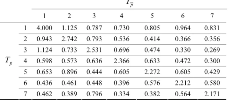
when lead-time mis-specification occurs, although it is asymptotically stable when the replenishment system is set up with correct lead-time information. Table 4 shows the effect of actual lead-time and perceived lead-time on the size of asymptotically stable region. It can be seen that when lead-time is perceived correctly (numbers on the main diagonal), the size of asymptotic stability is much bigger than those when lead-time information is incorrect (numbers above or below the diagonal). The importance of accurate lead-time information on asymptotic stability region is obvious.
5. Conclusion and discussion
This paper highlights the range of dynamic behaviours that are present in a constrained inventory system with only one constraint. It is interesting that even a simple deterministic model with a short lead-time is sufficient to generate such complex phenomena. We wonder what sort of impact stochastic models, longer lead-times, more constraints and multiple echelons will have? Compared to the character of the stable regions, the unstable regions are relatively unknown. We have shown that a complex and diversified set of behaviours and patterns exist in the unstable region. Managerially, in a supply chain or production setting, intuitively we may rank these classes of dynamic behaviours from good to bad as follows; asymptotic stability, periodicity, quasi-periodicity, chaos and divergence. The most surprising result we have revealed here is the fact that using wrong lead-time information in the EPVIOBPCS can
Fig. 7: Stability Comparison between (1-1) and (1-2).
Table 2: Change of dynamic behaviour in each region with Tp 1 and Tp changes observed in Fig. 7.
Tp = 1,Tp= 1 Tp = 1, Tp= 2 I Asymptotically stable Bounded Oscillation
II Asymptotically stable Divergent
III Bounded Oscillation Divergent
Fig. 8: Dynamic responses of Forbidden Returns EPVIOBPCS with a sudden increase of perceived lead-time under multiple parameter settings (verification of Fig. 7 and Table 2). (a) Region I: αS = 1.3, αSL = 1; (b) Region II: αS = 0.05,
Fig. 9: Stability Comparison between (2-2) and (2-1).
Table 3: Change of dynamic behaviour in each region with Tp 2 and Tp changes observed in Fig. 9.
Tp = 2,Tp= 2 Tp = 2, Tp= 1 I Asymptotically stable Bounded Oscillation
II Bounded Oscillation Asymptotically stable
III Divergent Asymptotically stable
Fig. 10: Dynamic responses of Forbidden Returns EPVIOBPCS with a sudden decrease of perceived lead-time under multiple parameter settings (verification of Fig. 9 and Table 3). (a) Region I: αS = 1.5, αSL = 1.2;
(b) Region II: αS = 0.1, αSL = -0.5; (c) Region III: αS = 0.05, αSL = -0.7; (d) Region IV: αS = 0.2, αSL = -1.2
Table 4: Size of the asymptotic stability region under different actual and perceived lead-times.
p T 1 2 3 4 5 6 7 1 4.000 1.125 0.787 0.730 0.805 0.964 0.831 2 0.943 2.742 0.793 0.536 0.414 0.366 0.356 3 1.124 0.733 2.531 0.696 0.474 0.330 0.269 4 0.598 0.573 0.636 2.366 0.633 0.472 0.300 5 0.653 0.896 0.444 0.605 2.272 0.605 0.429 6 0.436 0.461 0.448 0.396 0.576 2.212 0.580 p T 7 0.462 0.389 0.796 0.334 0.382 0.564 2.171
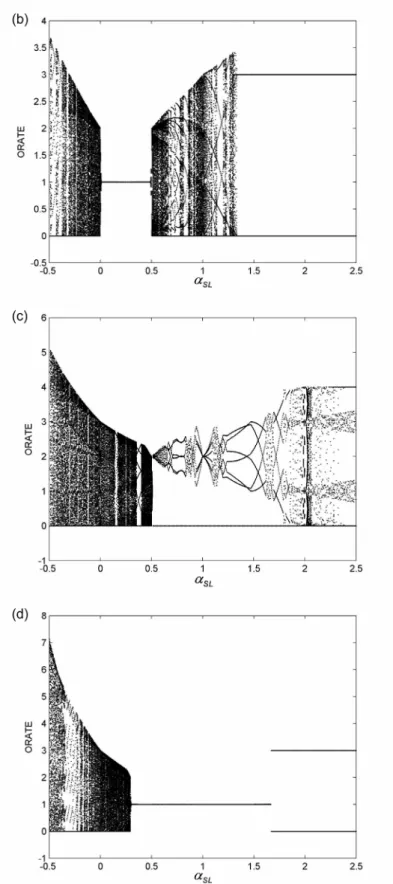
result in a periodic or a chaotic system. As the EPVIOBPCS is a general case of the Order-Up-To (OUT) policy this is a worrying result as the OUT policy is probably one of the most popular replenishment algorithms in industry. Fig. 11
takes another look at this issue by presenting four bifurcation diagrams, two with correct lead-times, two with
mis-specified lead-times. Fig. 11 was produced with MATLAB. For each bifurcation diagram, we run 500 simulation
experiments with the control parameter (αSL) changing. In each simulation the step response of ORATE for 1000
periods is generated and transient data in the first 800 periods is discarded. The remaining steady state data is then used to derive the bifurcation diagram. We see that the bifurcation criteria analytically obtained in Section 3 can be verified by these diagrams, and also the predicted complex and rich dynamic patterns can be observed, especially in (b) and (c). With incorrect lead-time information, the industrially prevalent OUT policy is not asymptotically stable. This
means that it is extremely important to obtain and use accurate lead-time information in a replenishment system. We also note that the estimated lead-time will affect system stability only in the EPVIOBPCS version of the OUT policy, which is designed to eliminate inventory drift. Hence, there might be a trade-off between effective inventory control and system stability. This requires more detailed investigation in the future. There is also a performance measurement / behaviour aspect to consider here. We have experience of a company where bonuses were awarded based on reductions in supplier lead-times. The information used to determine whether bonuses were awarded was gathered from the companies ERP system that was also used to schedule the production and coordinate the supply chain. Employees knew of this and covertly changed lead-time information in the ERP system without the subsequent physical reengineering efforts. The company was experiencing extreme dynamic behaviour in both production and inventory. We believe at least part of this dramatic dynamic behaviour can be explained by the phenomena described by this paper.
In this paper, we have adopted the assumption that the last observed demand is used as the forecast for the current period, i.e., Ta 1or α = 1, also known as the naïve forecasting method. This is acceptable in a step demand scenario as the forecast generated by the simple smoothing method (with Ta 0.5 to ensure stability) will eventually be equal to the demand. Using the naïve forecasting method only removes the transient response and does not affect the steady state. Furthermore, to obtain closed-form expressions of the stability criteria, we concentrated primarily on short lead-time scenarios, such as one or two periods. When longer lead-lead-times are present, the dynamic behaviour of the inventory system can be highly jeopardised; most importantly the asymptotic stability region will shrink in size as we
demonstrate in Table 4. Ordering policies with high inventory feedback and low WIP feedback are especially
vulnerable to lead-time increases. The Lyapunovian stability boundary moves to the right when lead-time increases, increasing the possibility of a divergent response. Meanwhile longer lead-times may increase the risk of lead-time errors being introduced, harming dynamic performance.
In the field of dynamical systems, the characterisation of high dimensional piecewise linear systems are far from being solved. Hence, to explore the dynamical behaviours of the constrained inventory system, a simulation-based technique has been incorporated with an eigenvalue analysis and knowledge of dynamical systems. Due to the unique nature of the Forbidden Returns system, a linear system stability analysis was sufficient to derive the asymptotic stability boundaries. However, in general this may not always be the case.
Acknowledgments
Xun Wang would like to thank the Chinese Scholarship Council for providing financial support (No. 2010602068) that enabled him to visit Cardiff University for 1 year. The support of National Natural Science Foundation of China (Nos. 70821061; 70872009; 71172016) is also acknowledged.
Fig. 11: Bifurcation diagrams for EPVIOBPCS when S = 1. (a) Case (1-1); (b) Case (1-2); (c) Case
(2-1); (d) Case (2-2)
References
Chaharsooghi, S.K., Heydari, J. (2010). Lead time variance or lead time mean reduction in supply chain management:
which one has a higher impact on supply chain performance? International Journal of Production Economics,
Cheema, P.S. (1994). Dynamic analysis of and inventory and production control system with an adaptive lead-time estimator, Ph.D. Dissertation, Cardiff University, UK.
Coleman, J.C. (1988). Lead time reduction for system simplification, M.Sc. Dissertation, Cardiff University, UK. Dejonckheere, J., Disney, S.M., Lambrecht, M.R. and Towill, D.R. (2003). Measuring and avoiding the bullwhip
effect: A control theoretic approach. European Journal of Operational Research, 147, (3), 567-590.
Disney, S.M., Towill, D.R. (2003). On the bullwhip and inventory variance produced by an ordering policy. Omega,
31, 157-167.
Disney, S.M., Towill, D.R. (2005). Eliminating drift in inventory and order based production control systems.
International Journal of Production Economics, 93-94, 331-344.
Disney, S.M. (2008). Supply chain aperiodicity, bullwhip and stability analysis with Jury’s Inners. IMA Journal of
Management Mathematics, 19, 101-116.
Edghill, J.S., Towill, D.R. (1989). The use of systems dynamics in manufacturing systems. Transaction of the Institute of Measurement and Control, 11, 208–216.
Forrester, J.W. (1961). Industrial dynamics. Cambridge: MIT Press and New York: Wiley.
Hosoda, T., Disney, S.M. (2009). Impact of market demand mis-specification on a two-level supply chain.
International Journal of Production Economics, 121, 739-751.
Hwarng, H.B., Xie, N. (2008). Understanding supply chain dynamics: a chaos perspective. European Journal of
Operational Research, 184, 1163-1178.
John, S., Naim, M.M., Towill, D.R. (1994). Dynamic analysis of a WIP compensated decision support system.
International Journal of Manufacturing System Design, 1, 283-297.
Jury, E.I. (1974). Inners and the stability of dynamic systems. John Wiley, New York.
Kim, J.G., Chatfield, D., Harrison, T.P., & Hayya, J.C. (2006). Quantifying the bullwhip effect in a supply chain with stochastic lead time. European Journal of Operational Research, 173, 17-636.
Larsen, E.R., Morecroft, J.D.W., Thomsen, J.S. (1999). Complex behaviour in a production-distribution model.
European Journal of Operational Research, 119, 61-74.
Laugessen, J., Mosekilde, E. (2006). Border-collision bifurcations in a dynamic management game. Computers &
Operations Research, 33, 464-478.
Liu, H. (2005). Research on dynamics of supply chain, Ph.D. Dissertation, Huazhong University of Science and Technology, P.R. China.
Mosekilde, E., Larsen, E.R. (1988). Deterministic chaos in the beer production distribution model. System Dynamics Review, 4, 131-147.
Mosekilde, E., Laugessen, J. (2007). Non-linear dynamic phenomena in the beer model. System Dynamics Review, 23, 229-252.
Nagatani, T., Helbing, D. (2004). Stability analysis and stabilization strategies for linear supply chains, Physica A, 335, 644-660.
Riddalls, C.E., Bennett, S., Tipi, N.S. (2000). Modelling the dynamics of supply chains. International Journal of
Systems Science, 31, 969-976.
Riddalls, C.E., Bennett, S. (2002). The stability of supply chains. International Journal of Production Research, 40, 459-475.
Rodrigues, L., Boukas, E. (2006). Piecewise-linear H∞ controller synthesis with applications to inventory control of switched production systems. Automatica, 42, 1245-1254.
Rossi, R., Tarim, S.A., Hnich, B., & Prestwich, S. (2010). Computing the non-stationary replenishment cycle inventory policy under stochastic supplier lead-times. International Journal of Production Economics, 127, 180-189.
Sarimveis, H., Patrinos, P., Tarantilis, C.D., & Kiranoudis, C.T. (2008). Dynamic modelling and control of supply chain systems: A review. Computers & Operations Research, 35, 3530-3561.
Simon, H.A. (1952). On the application of servomechanism theory in the study of production control. Econometrica,
20, 247-268.
Sun, Z. (2010). Stability of piecewise linear systems revisited. Annual Reviews in Control, 34, 221-231.
Thomsen, J.S., Mosekilde, E., Sterman, J.D. (1992). Hyperchaotic phenomena in dynamic decision making. System
Analysis and Modelling Simulation, 9, 137-156.
Towill, D.R. (1982). Dynamic analysis of an inventory and order based production control system. International
Journal of Production Research, 20, 671-687.
Wang, K.J., Wee, H.M., Gao, S.F., & Chung, S.L. (2005). Production and inventory control with chaotic demands.
Omega, 33, 97-106.
Warburton, R.D.H., Disney, S.M., Towill, D.R., & Hodgson, J.P.E. (2004). Further insights into “The stability of supply chains". International Journal of Production Research, 42, 639-648.
Wu, Y., Zhang, D.Z. (2007). Demand fluctuation and chaotic behaviour by interaction between customers and suppliers. International Journal of Production Economics, 107, 250-259.