John Duchi [email protected] Google, Mountain View, CA 94043
Shai Shalev-Shwartz [email protected]
Toyota Technological Institute, Chicago, IL, 60637
Yoram Singer [email protected]
Tushar Chandra [email protected]
Google, Mountain View, CA 94043
Abstract
We describe efficient algorithms for projecting a vector onto theℓ1-ball. We present two methods
for projection. The first performs exact projec-tion in O(n)expected time, where nis the di-mension of the space. The second works on vec-tors k of whose elements are perturbed outside theℓ1-ball, projecting inO(klog(n))time. This
setting is especially useful for online learning in sparse feature spaces such as text categorization applications. We demonstrate the merits and ef-fectiveness of our algorithms in numerous batch and online learning tasks. We show that vari-ants of stochastic gradient projection methods augmented with our efficient projection proce-dures outperform interior point methods, which are considered state-of-the-art optimization tech-niques. We also show that in online settings gra-dient updates withℓ1projections outperform the
exponentiated gradient algorithm while obtain-ing models with high degrees of sparsity.
1. Introduction
A prevalent machine learning approach for decision and prediction problems is to cast the learning task as penal-ized convex optimization. In penalpenal-ized convex optimiza-tion we seek a set of parameters, gathered together in a vectorw, which minimizes a convex objective function in w with an additional penalty term that assesses the
com-plexity of w. Two commonly used penalties are the
1-norm and the square of the 2-1-norm of w. An alternative Appearing in Proceedings of the25thInternational Conference
on Machine Learning, Helsinki, Finland, 2008. Copyright 2008
by the author(s)/owner(s).
but mathematically equivalent approach is to cast the prob-lem as a constrained optimization probprob-lem. In this setting we seek a minimizer of the objective function while con-straining the solution to have a bounded norm. Many re-cent advances in statistical machine learning and related fields can be explained as convex optimization subject to a 1-norm constraint on the vector of parameters w.
Im-posing anℓ1 constraint leads to notable benefits. First, it
encourages sparse solutions, i.e a solution for which many components ofware zero. When the original dimension
of w is very high, a sparse solution enables easier
inter-pretation of the problem in a lower dimension space. For the usage ofℓ1-based approach in statistical machine
learn-ing see for example (Tibshirani, 1996) and the references therein. Donoho (2006b) provided sufficient conditions for obtaining an optimalℓ1-norm solution which is sparse.
Re-cent work on compressed sensing (Candes, 2006; Donoho, 2006a) further explores howℓ1constraints can be used for
recovering a sparse signal sampled below the Nyquist rate. The second motivation for usingℓ1constraints in machine
learning problems is that in some cases it leads to improved generalization bounds. For example, Ng (2004) examined the task of PAC learning a sparse predictor and analyzed cases in which an ℓ1 constraint results in better solutions
than anℓ2constraint.
In this paper we re-examine the task of minimizing a con-vex function subject to an ℓ1 constraint on the norm of
the solution. We are particularly interested in cases where the convex function is the average loss over a training set of mexamples where each example is represented as a vector of high dimension. Thus, the solution itself is a high-dimensional vector as well. Recent work on ℓ2
constrained optimization for machine learning indicates that gradient-related projection algorithms are more effi-cient in approaching a solution of good generalization than second-order algorithms when the number of examples and
the dimension are large. For instance, Shalev-Shwartz et al. (2007) give recent state-of-the-art methods for solv-ing large scale support vector machines. Adaptsolv-ing these recent results to projection methods onto theℓ1ball poses
algorithmic challenges. While projections ontoℓ2balls are
straightforward to implement in linear time with the ap-propriate data structures, projection onto an ℓ1 ball is a
more involved task. The main contribution of this paper is the derivation of gradient projections withℓ1domain
con-straints that can be performed almost as fast as gradient projection withℓ2constraints.
Our starting point is an efficient method for projection onto the probabilistic simplex. The basic idea is to show that, after sorting the vector we need to project, it is possible to calculate the projection exactly in linear time. This idea was rediscovered multiple times. It was first described in an abstract and somewhat opaque form in the work of Gafni and Bertsekas (1984) and Bertsekas (1999). Crammer and Singer (2002) rediscovered a similar projection algorithm as a tool for solving the dual of multiclass SVM. Hazan (2006) essentially reuses the same algorithm in the con-text of online convex programming. Our starting point is another derivation of Euclidean projection onto the sim-plex that paves the way to a few generalizations. First we show that the same technique can also be used for project-ing onto theℓ1-ball. This algorithm is based on sorting the
components of the vector to be projected and thus requires
O(nlog(n))time. We next present an improvement of the algorithm that replaces sorting with a procedure resembling median-search whose expected time complexity isO(n). In many applications, however, the dimension of the feature space is very high yet the number of features which attain non-zero values for an example may be very small. For in-stance, in our experiments with text classification in Sec. 7, the dimension is two million (the bigram dictionary size) while each example has on average one-thousand non-zero features (the number of unique tokens in a document). Ap-plications where the dimensionality is high yet the number of “on” features in each example is small render our second algorithm useless in some cases. We therefore shift gears and describe a more complex algorithm that employs red-black trees to obtain a linear dependence on the number of non-zero features in an example and only logarithmic dependence on the full dimension. The key to our con-struction lies in the fact that we project vectors that are the sum of a vector in theℓ1-ball and a sparse vector—they are
“almost” in theℓ1-ball.
In conclusion to the paper we present experimental results that demonstrate the merits of our algorithms. We compare our algorithms with several specialized interior point (IP) methods as well as general methods from the literature for solvingℓ1-penalized problems on both synthetic and real
data (the MNIST handwritten digit dataset and the Reuters RCV1 corpus) for batch and online learning. Our projec-tion based methods outperform competing algorithms in terms of sparsity, and they exhibit faster convergence and lower regret than previous methods.
2. Notation and Problem Setting
We start by establishing the notation used throughout the paper. The set of integers 1through nis denoted by[n]. Scalars are denoted by lower case letters and vectors by lower case bold face letters. We use the notationw ≻ b
to designate that all of the components of w are greater
thanb. We usek · kas a shorthand for the Euclidean norm
k·k2. The other norm we use throughout the paper is the
1-norm of the vector,kvk1=Pni=1|vi|. Lastly, we consider order statistics and sorting vectors frequently throughout this paper. To that end, we let v(i) denote theith order
statistic ofv, that is,v(1) ≥v(2)≥. . .≥v(n)forv∈Rn.
In the setting considered in this paper we are provided with a convex functionL : Rn → R. Our goal is to find the minimum ofL(w)subject to anℓ1-norm constraint onw.
Formally, the problem we need to solve is minimize
w
L(w) s.t. kwk1≤z . (1)
Our focus is on variants of the projected subgradient method for convex optimization (Bertsekas, 1999). Pro-jected subgradient methods minimize a functionL(w)
sub-ject to the constraint thatw∈X, forX convex, by
gener-ating the sequence{w(t)}via w(t+1)= ΠX
w(t)−ηt∇(t)
(2) where ∇(t) is (an unbiased estimate of) the (sub)gradient
of L at w(t) and ΠX(x) = argminy{kx−yk | y ∈
X}is Euclidean projection ofxontoX. In the rest of the
paper, the main algorithmic focus is on the projection step (computing an unbiased estimate of the gradient ofL(w)is
straightforward in the applications considered in this paper, as is the modification ofw(t)by∇(t)).
3. Euclidean Projection onto the Simplex
For clarity, we begin with the task of performing Euclidean projection onto the positive simplex; our derivation natu-rally builds to the more efficient algorithms. As such, the most basic projection task we consider can be formally de-scribed as the following optimization problem,minimize w 1 2kw−vk 2 2 s.t. n X i=1 wi = z , wi≥0 . (3)
Whenz = 1the above is projection onto the probabilistic simplex. The Lagrangian of the problem in Eq. (3) is
L(w,ζ) = 1 2kw−vk 2+θ n X i=1 wi−z ! −ζ·w ,
where θ ∈ Ris a Lagrange multiplier andζ ∈ Rn+ is a
vector of non-negative Lagrange multipliers. Differenti-ating with respect to wi and comparing to zero gives the optimality condition, dwdL
i = wi −vi +θ−ζi = 0.
The complementary slackness KKT condition implies that whenever wi > 0 we must have that ζi = 0. Thus, if
wi>0we get that
wi = vi−θ+ζi = vi−θ . (4) All the non-negative elements of the vectorware tied via
a single variable, so knowing the indices of these elements gives a much simpler problem. Upon first inspection, find-ing these indices seems difficult, but the followfind-ing lemma (Shalev-Shwartz & Singer, 2006) provides a key tool in de-riving our procedure for identifying non-zero elements. Lemma 1. Letwbe the optimal solution to the
minimiza-tion problem in Eq. (3). Letsand j be two indices such
thatvs> vj. Ifws= 0thenwjmust be zero as well. Denoting byI the set of indices of the non-zero compo-nents of the sorted optimal solution,I ={i∈[n] :v(i) >
0}, we see that Lemma 1 implies thatI = [ρ] for some 1 ≤ρ≤n. Had we knownρwe could have simply used Eq. (4) to obtain that
n X i=1 wi= n X i=1 w(i)= ρ X i=1 w(i)= ρ X i=1 v(i)−θ=z and therefore θ= 1 ρ ρ X i=1 v(i)−z ! . (5)
Givenθwe can characterize the optimal solution forwas wi = max{vi−θ , 0} . (6) We are left with the problem of finding the optimalρ, and the following lemma (Shalev-Shwartz & Singer, 2006) pro-vides a simple solution once we sortvin descending order.
Lemma 2. Letwbe the optimal solution to the
minimiza-tion problem given in Eq. (3). Letµdenote the vector
ob-tained by sortingvin a descending order. Then, the
num-ber of strictly positive elements inwis
ρ(z,µ) = max ( j∈[n] : µj− 1 j j X r=1 µr−z ! >0 ) .
The pseudo-code describing theO(nlogn)procedure for solving Eq. (3) is given in Fig. 1.
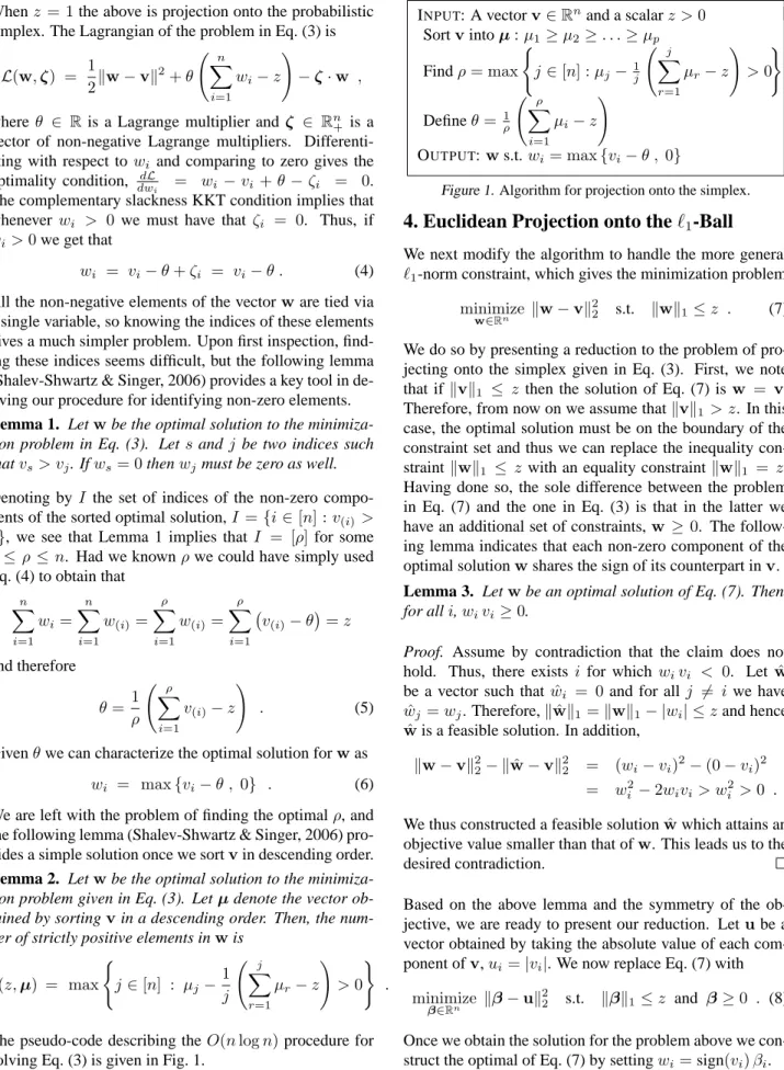
INPUT: A vectorv∈Rnand a scalarz >0
Sortvintoµ:µ1≥µ2≥. . .≥µp Findρ= max ( j ∈[n] :µj−1j j X r=1 µr−z ! >0 ) Defineθ= 1ρ ρ X i=1 µi−z ! OUTPUT:ws.t.wi= max{vi−θ , 0}
Figure 1. Algorithm for projection onto the simplex.
4. Euclidean Projection onto the
ℓ
1-Ball
We next modify the algorithm to handle the more generalℓ1-norm constraint, which gives the minimization problem
minimize
w∈Rn kw−vk
2
2 s.t. kwk1≤z . (7)
We do so by presenting a reduction to the problem of pro-jecting onto the simplex given in Eq. (3). First, we note that ifkvk1 ≤ z then the solution of Eq. (7) isw = v.
Therefore, from now on we assume thatkvk1> z. In this
case, the optimal solution must be on the boundary of the constraint set and thus we can replace the inequality con-straintkwk1 ≤ z with an equality constraintkwk1 = z.
Having done so, the sole difference between the problem in Eq. (7) and the one in Eq. (3) is that in the latter we have an additional set of constraints,w ≥0. The
follow-ing lemma indicates that each non-zero component of the optimal solutionwshares the sign of its counterpart inv.
Lemma 3. Letwbe an optimal solution of Eq. (7). Then,
for alli,wivi≥0.
Proof. Assume by contradiction that the claim does not
hold. Thus, there exists i for which wivi < 0. Let wˆ
be a vector such thatwˆi = 0and for all j 6= i we have ˆ
wj=wj. Therefore,kwˆk1=kwk1− |wi| ≤zand hence ˆ
wis a feasible solution. In addition,
kw−vk22− kwˆ −vk22 = (wi−vi)2−(0−vi)2
= w2i −2wivi> wi2>0 . We thus constructed a feasible solutionwˆ which attains an objective value smaller than that ofw. This leads us to the
desired contradiction.
Based on the above lemma and the symmetry of the ob-jective, we are ready to present our reduction. Letube a
vector obtained by taking the absolute value of each com-ponent ofv,ui=|vi|. We now replace Eq. (7) with
minimize
β∈Rn kβ−uk
2
2 s.t. kβk1≤z and β≥0 . (8)
Once we obtain the solution for the problem above we con-struct the optimal of Eq. (7) by settingwi=sign(vi)βi.
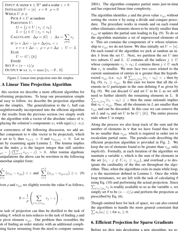
INPUTA vectorv∈Rnand a scalarz >0 INITIALIZEU = [n] s= 0 ρ= 0 WHILEU 6=φ PICKk∈Uat random PARTITIONU: G={j∈U |vj ≥vk} L={j∈U |vj< vk} CALCULATE ∆ρ=|G| ; ∆s=X j∈G vj IF(s+ ∆s)−(ρ+ ∆ρ)vk< z s=s+ ∆s ; ρ=ρ+ ∆ρ ; U ←L ELSE U ←G\ {k} ENDIF SETθ= (s−z)/ρ OUTPUTws.t.vi= max{vi−θ , 0}
Figure 2. Linear time projection onto the simplex.
5. A Linear Time Projection Algorithm
In this section we describe a more efficient algorithm for performing projections. To keep our presentation simple and easy to follow, we describe the projection algorithm onto the simplex. The generalization to the ℓ1 ball can
straightforwardly incorporated into the efficient algorithm by the results from the previous section (we simply work in the algorithm with a vector of the absolute values ofv,
replacing the solution’s componentswiwith sign(vi)·wi). For correctness of the following discussion, we add an-other component tov (the vector to be projected), which
we set to 0, thus vn+1 = 0 and v(n+1) = 0. Let us
start by examining again Lemma 2. The lemma implies that the index ρ is the largest integer that still satisfies
v(ρ) − 1ρ Pρr=1v(r)−z
> 0. After routine algebraic manipulations the above can be rewritten in the following somewhat simpler form:
ρ X i=1 v(i)−v(ρ) < z and ρ+1 X i=1 v(i)−v(ρ+1) ≥z. (9)
Givenρandv(ρ)we slightly rewrite the valueθas follows,
θ=1 ρ X j:vj≥v(ρ) vj−z . (10)
The task of projection can thus be distilled to the task of findingθ, which in turn reduces to the task of findingρand the pivot element v(ρ). Our problem thus resembles the
task of finding an order statistic with an additional compli-cating factor stemming from the need to compute summa-tions (while searching) of the form given by Eq. (9). Our efficient projection algorithm is based on a modification of the randomized median finding algorithm (Cormen et al.,
2001). The algorithm computes partial sums just-in-time and has expected linear time complexity.
The algorithm identifiesρand the pivot valuev(ρ)without
sorting the vectorvby using a divide and conquer
proce-dure. The procedure works in rounds and on each round either eliminates elements shown to be strictly smaller than
v(ρ)or updates the partial sum leading to Eq. (9). To do so
the algorithm maintains a set of unprocessed elements of
v. This set contains the components ofvwhose
relation-ship tov(ρ)we do not know. We thus initially setU = [n].
On each round of the algorithm we pick at random an in-dex k from the setU. Next, we partition the set U into two subsetsGandL. Gcontains all the indices j ∈ U
whose componentsvj > vk;Lcontains thosej ∈U such that vj is smaller. We now face two cases related to the current summation of entries invgreater than the
hypoth-esized v(ρ)(i.e. vk). IfPj:vj≥vk(vj −vk) < zthen by
Eq. (9),vk ≥ v(ρ). In this case we know that all the
el-ements inGparticipate in the sum definingθas given by Eq. (9). We can discard Gand setU to beL as we still need to further identify the remaining elements in L. If
P
j:vj≥vk(vj −vk) ≥ z then the same rationale implies
thatvk < v(ρ). Thus, all the elements inLare smaller than
v(ρ)and can be discarded. In this case we can remove the
setLandvk and setU to beG\ {k}. The entire process ends whenU is empty.
Along the process we also keep track of the sum and the number of elements in v that we have found thus far to
be no smaller thanv(ρ), which is required in order not to
recalculate partial sums. The pseudo-code describing the efficient projection algorithm is provided in Fig. 2. We keep the set of elements found to be greater thanv(ρ)only
implicitly. Formally, at each iteration of the algorithm we
maintain a variables, which is the sum of the elements in the set {vj : j 6∈ U, vj ≥ v(ρ)}, and overloadρto
des-ignate the cardinality of the this set throughout the algo-rithm. Thus, when the algorithms exits its main while loop,
ρis the maximizer defined in Lemma 1. Once the while loop terminates, we are left with the task of calculatingθ
using Eq. (10) and performing the actual projection. Since
P
j:vj≥µρvj is readily available to us as the variables, we
simply setθto be(s−z)/ρand perform the projection as prescribed by Eq. (6).
Though omitted here for lack of space, we can also extend the algorithms to handle the more general constraint that
Pa
i|wi| ≤zforai≥0.
6. Efficient Projection for Sparse Gradients
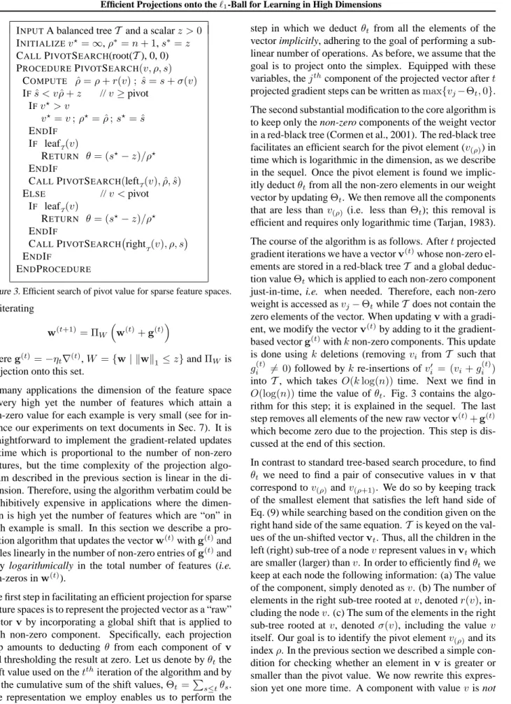
Before we dive into developing a new algorithm, we re-mind the reader of the iterations the minimization algo-rithm takes from Eq. (2): we generate a sequence{w(t)}INPUTA balanced treeT and a scalarz >0 INITIALIZEv⋆=∞,ρ∗=n+ 1,s∗=z CALLPIVOTSEARCH(root(T), 0, 0) PROCEDUREPIVOTSEARCH(v, ρ, s)
COMPUTE ρˆ=ρ+r(v) ; ˆs=s+σ(v) IFˆs < vρˆ+z //v≥pivot IFv⋆> v v⋆=v;ρ⋆= ˆρ;s⋆= ˆs ENDIF IF leafT(v) RETURN θ= (s⋆−z)/ρ⋆ ENDIF
CALLPIVOTSEARCH(leftT(v),ρ,ˆsˆ)
ELSE //v <pivot
IF leafT(v)
RETURN θ= (s⋆−z)/ρ⋆ ENDIF
CALLPIVOTSEARCH right
T(v), ρ, s
ENDIF
ENDPROCEDURE
Figure 3. Efficient search of pivot value for sparse feature spaces.
by iterating w(t+1)= ΠW w(t)+g(t) whereg(t)=−ηt∇(t),W ={w| kwk1≤z}andΠW is
projection onto this set.
In many applications the dimension of the feature space is very high yet the number of features which attain a non-zero value for each example is very small (see for in-stance our experiments on text documents in Sec. 7). It is straightforward to implement the gradient-related updates in time which is proportional to the number of non-zero features, but the time complexity of the projection algo-rithm described in the previous section is linear in the di-mension. Therefore, using the algorithm verbatim could be prohibitively expensive in applications where the dimen-sion is high yet the number of features which are “on” in each example is small. In this section we describe a pro-jection algorithm that updates the vectorw(t)withg(t)and
scales linearly in the number of non-zero entries ofg(t)and
only logarithmically in the total number of features (i.e. non-zeros inw(t)).
The first step in facilitating an efficient projection for sparse feature spaces is to represent the projected vector as a “raw” vectorv by incorporating a global shift that is applied to
each non-zero component. Specifically, each projection step amounts to deducting θ from each component of v
and thresholding the result at zero. Let us denote byθtthe shift value used on thetthiteration of the algorithm and by Θtthe cumulative sum of the shift values,Θt=Ps≤tθs. The representation we employ enables us to perform the
step in which we deduct θt from all the elements of the vector implicitly, adhering to the goal of performing a sub-linear number of operations. As before, we assume that the goal is to project onto the simplex. Equipped with these variables, thejthcomponent of the projected vector aftert projected gradient steps can be written asmax{vj−Θt,0}. The second substantial modification to the core algorithm is to keep only the non-zero components of the weight vector in a red-black tree (Cormen et al., 2001). The red-black tree facilitates an efficient search for the pivot element (v(ρ)) in
time which is logarithmic in the dimension, as we describe in the sequel. Once the pivot element is found we implic-itly deductθtfrom all the non-zero elements in our weight vector by updatingΘt. We then remove all the components that are less than v(ρ)(i.e. less than Θt); this removal is
efficient and requires only logarithmic time (Tarjan, 1983). The course of the algorithm is as follows. Aftertprojected gradient iterations we have a vectorv(t)whose non-zero
el-ements are stored in a red-black treeT and a global deduc-tion valueΘtwhich is applied to each non-zero component just-in-time, i.e. when needed. Therefore, each non-zero weight is accessed asvj−ΘtwhileT does not contain the zero elements of the vector. When updatingvwith a
gradi-ent, we modify the vectorv(t)by adding to it the
gradient-based vectorg(t)withknon-zero components. This update
is done usingk deletions (removingvi fromT such that
gi(t) 6= 0) followed bykre-insertions ofv′
i = (vi+gi(t)) into T, which takes O(klog(n)) time. Next we find in
O(log(n))time the value ofθt. Fig. 3 contains the algo-rithm for this step; it is explained in the sequel. The last step removes all elements of the new raw vectorv(t)+g(t)
which become zero due to the projection. This step is dis-cussed at the end of this section.
In contrast to standard tree-based search procedure, to find
θt we need to find a pair of consecutive values inv that
correspond tov(ρ)andv(ρ+1). We do so by keeping track
of the smallest element that satisfies the left hand side of Eq. (9) while searching based on the condition given on the right hand side of the same equation.T is keyed on the val-ues of the un-shifted vectorvt. Thus, all the children in the left (right) sub-tree of a nodevrepresent values invtwhich are smaller (larger) thanv. In order to efficiently findθtwe keep at each node the following information: (a) The value of the component, simply denoted asv. (b) The number of elements in the right sub-tree rooted atv, denotedr(v), in-cluding the nodev. (c) The sum of the elements in the right sub-tree rooted atv, denotedσ(v), including the valuev
itself. Our goal is to identify the pivot elementv(ρ)and its
indexρ. In the previous section we described a simple con-dition for checking whether an element invis greater or
smaller than the pivot value. We now rewrite this expres-sion yet one more time. A component with valuev is not
smaller than the pivot iff the following holds:
X
j:vj≥v
vj>|{j:vj ≥v}| ·v+z . (11)
The variables in the red-black tree form the infrastructure for performing efficient recursive computation of Eq. (11). Note also that the condition expressed in Eq. (11) still holds when we do not deductΘtfrom all the elements inv.
The search algorithm maintains recursively the numberρ
and the sumsof the elements that have been shown to be greater or equal to the pivot. We start the search with the root node ofT, and thus initiallyρ= 0ands= 0. Upon entering a new nodev, the algorithm checks whether the condition given by Eq. (11) holds forv. Sinceρandswere computed for the parent ofv, we need to incorporate the number and the sum of the elements that are larger thanv
itself. By construction, these variables arer(v)andσ(v), which we store at the nodev itself. We letρˆ=ρ+r(v) andsˆ=s+σ(v), and with these variables handy, Eq. (11) distills to the expressions < vˆ ρˆ+z. If the inequality holds, we know thatvis either larger than the pivot or it may be the pivot itself. We thus update our current hypothesis for
µρandρ(designated asv⋆andρ⋆in Fig. 3). We continue searching the left sub-tree (leftT(v)) which includes all el-ements smaller thanv. If inequalitys < vˆ ρˆ+zdoes not hold, we know thatv < µρ, and we thus search the right subtree (right
T(v)) and keepρandsintact. The process
naturally terminates once we reach a leaf, where we can also calculate the correct value ofθusing Eq. (10). Once we find θt (ifθt ≥ 0) we update the global shift, Θt+1 = Θt+θt. We need to discard all the elements in
T smaller thanΘt+1, which we do using Tarjan’s (1983)
algorithm for splitting a red-black tree. This step is log-arithmic in the total number of non-zero elements of vt. Thus, as the additional variables in the tree can be updated in constant time as a function of a node’s child nodes in
T, each of the operations previously described can be per-formed in logarthmic time (Cormen et al., 2001), giving us a total update time ofO(klog(n)).
7. Experiments
We now present experimental results demonstrating the ef-fectiveness of the projection algorithms. We first report re-sults for experiments with synthetic data and then move to experiments with high dimensional natural datasets. In our experiment with synthetic data, we compared vari-ants of the projected subgradient algorithm (Eq. (2)) for
ℓ1-regularized least squares andℓ1-regularized logistic
re-gression. We compared our methods to a specialized coordinate-descent solver for the least squares problem due to Friedman et al. (2007) and to very fast interior point
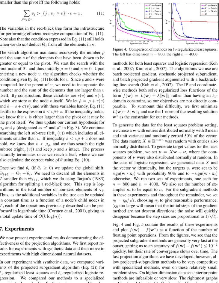
0.2 0.4 0.6 0.8 1 1.2 1.4 1.6 1.8 2 2.2 x 10⁸ 10−1 100 101 102 Approximate Flops f − f * Coordinate L1 − Line L1 − Batch L1 − Stoch IP 1 2 3 4 5 6 x 10⁹ 10−1 100 101 102 103 Approximate Flops f − f * Coordinate L1 − Batch L1 − Stoch IP
Figure 4. Comparison of methods onℓ1-regularized least squares. The left has dimensionn= 800, the rightn= 4000
methods for both least squares and logistic regression (Koh et al., 2007; Kim et al., 2007). The algorithms we use are batch projected gradient, stochastic projected subgradient, and batch projected gradient augmented with a backtrack-ing line search (Koh et al., 2007). The IP and coordinate-wise methods both solve regularized loss functions of the form f(w) = L(w) +λkwk1 rather than having anℓ1
-domain constraint, so our objectives are not directly com-parable. To surmount this difficulty, we first minimize
L(w)+λkwk1and use the 1-norm of the resulting solution
w∗as the constraint for our methods.
To generate the data for the least squares problem setting, we chose awwith entries distributed normally with 0 mean
and unit variance and randomly zeroed 50% of the vector. The data matrixX ∈Rm×n was random with entries also normally distributed. To generate target values for the least squares problem, we sety = Xw+ν, where the
com-ponents ofνwere also distributed normally at random. In the case of logistic regression, we generated data X and the vector w identically, but the targetsyi were set to be sign(w·xi)with probability 90% and to −sign(w ·xi)
otherwise. We ran two sets of experiments, one each for
n = 800andn = 4000. We also set the number of ex-amples mto be equal ton. For the subgradient methods in these experiments and throughout the remainder, we set
ηt=η0/
√
t, choosingη0to give reasonable performance.
(η0too large will mean that the initial steps of the gradient
method are not descent directions; the noise will quickly disappear because the step sizes are proportional to1/√t). Fig. 4 and Fig. 5 contain the results of these experiments and plot f(w)−f(w∗) as a function of the number of
floating point operations. From the figures, we see that the projected subgradient methods are generally very fast at the outset, getting us to an accuracy off(w)−f(w∗)≤10−2
quickly, but their rate of convergence slows over time. The fast projection algorithms we have developed, however, al-low projected-subgradient methods to be very competitive with specialized methods, even on these relatively small problem sizes. On higher-dimension data sets interior point methods are infeasible or very slow. The rightmost graphs in Fig. 4 and Fig. 5 plot f(w)−f(w∗)as functions of
re-0.5 1 1.5 2 2.5 3 3.5 4 4.5 5 5.5 x 10⁸ 10−4 10−3 10−2 10−1 Approximate Flops f − f * L1 − Line L1 − Batch L1 − Stoch IP 1 2 3 4 5 6 7 8 x 10⁹ 10−5 10−4 10−3 10−2 10−1 Approximate Flops f − f * L1 − Batch L1 − Stoch IP
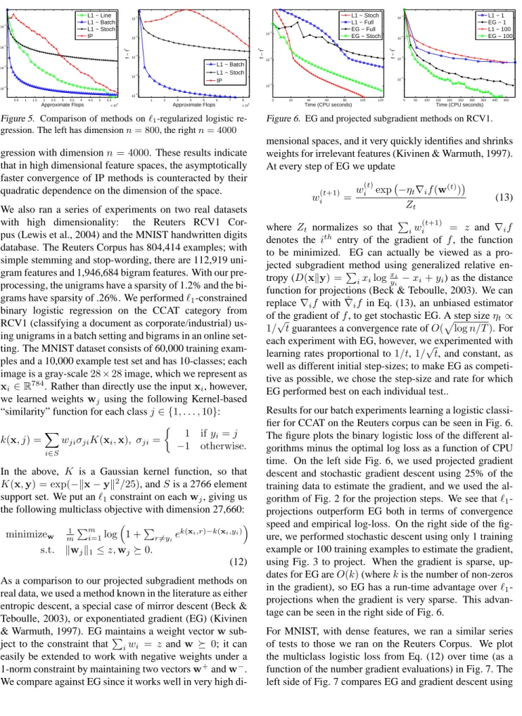
Figure 5. Comparison of methods onℓ1-regularized logistic re-gression. The left has dimensionn= 800, the rightn= 4000
gression with dimensionn= 4000. These results indicate that in high dimensional feature spaces, the asymptotically faster convergence of IP methods is counteracted by their quadratic dependence on the dimension of the space. We also ran a series of experiments on two real datasets with high dimensionality: the Reuters RCV1 Cor-pus (Lewis et al., 2004) and the MNIST handwritten digits database. The Reuters Corpus has 804,414 examples; with simple stemming and stop-wording, there are 112,919 uni-gram features and 1,946,684 biuni-gram features. With our pre-processing, the unigrams have a sparsity of 1.2% and the bi-grams have sparsity of .26%. We performedℓ1-constrained
binary logistic regression on the CCAT category from RCV1 (classifying a document as corporate/industrial) us-ing unigrams in a batch settus-ing and bigrams in an online set-ting. The MNIST dataset consists of 60,000 training exam-ples and a 10,000 example test set and has 10-classes; each image is a gray-scale28×28image, which we represent as
xi ∈R784. Rather than directly use the inputxi, however, we learned weights wj using the following Kernel-based “similarity” function for each classj∈ {1, . . . ,10}:
k(x, j) =X i∈S wjiσjiK(xi,x), σji= 1 if yi=j −1 otherwise.
In the above, K is a Gaussian kernel function, so that
K(x,y) = exp(−kx−yk2/25), andSis a 2766 element
support set. We put anℓ1constraint on eachwj, giving us the following multiclass objective with dimension 27,660:
minimizew 1 m Pm i=1log 1 +P r6=yie k(xi,r)−k(xi,yi) s.t. kwjk1≤z,wj 0. (12) As a comparison to our projected subgradient methods on real data, we used a method known in the literature as either entropic descent, a special case of mirror descent (Beck & Teboulle, 2003), or exponentiated gradient (EG) (Kivinen & Warmuth, 1997). EG maintains a weight vectorw
sub-ject to the constraint that P
iwi = z andw 0; it can
easily be extended to work with negative weights under a 1-norm constraint by maintaining two vectorsw+andw−.
We compare against EG since it works well in very high
di-0 20 40 60 80 100 120 10−3
10−2
10−1
Time (CPU seconds)
f − f * L1 − Stoch L1 − Full EG − Full EG − Stoch 0 50 100 150 200 250 300 350 400 450 10−4 10−3 10−2 10−1
Time (CPU seconds)
f − f * L1 − 1 EG − 1 L1 − 100 EG − 100
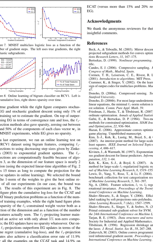
Figure 6. EG and projected subgradient methods on RCV1.
mensional spaces, and it very quickly identifies and shrinks weights for irrelevant features (Kivinen & Warmuth, 1997). At every step of EG we update
w(it+1)= w
(t)
i exp −ηt∇if(w(t)) Zt
(13) where Zt normalizes so that Piw
(t+1)
i = z and ∇if denotes the ith entry of the gradient of f, the function to be minimized. EG can actually be viewed as a pro-jected subgradient method using generalized relative en-tropy (D(xky) =Pixilogxyii −xi+yi) as the distance function for projections (Beck & Teboulle, 2003). We can replace∇if with∇ˆif in Eq. (13), an unbiased estimator of the gradient off, to get stochastic EG. A step sizeηt∝ 1/√tguarantees a convergence rate ofO(p
logn/T). For each experiment with EG, however, we experimented with learning rates proportional to1/t,1/√t, and constant, as well as different initial step-sizes; to make EG as competi-tive as possible, we chose the step-size and rate for which EG performed best on each individual test..
Results for our batch experiments learning a logistic classi-fier for CCAT on the Reuters corpus can be seen in Fig. 6. The figure plots the binary logistic loss of the different al-gorithms minus the optimal log loss as a function of CPU time. On the left side Fig. 6, we used projected gradient descent and stochastic gradient descent using 25% of the training data to estimate the gradient, and we used the al-gorithm of Fig. 2 for the projection steps. We see thatℓ1
-projections outperform EG both in terms of convergence speed and empirical log-loss. On the right side of the fig-ure, we performed stochastic descent using only 1 training example or 100 training examples to estimate the gradient, using Fig. 3 to project. When the gradient is sparse, up-dates for EG areO(k)(wherekis the number of non-zeros in the gradient), so EG has a run-time advantage overℓ1
-projections when the gradient is very sparse. This advan-tage can be seen in the right side of Fig. 6.
For MNIST, with dense features, we ran a similar series of tests to those we ran on the Reuters Corpus. We plot the multiclass logistic loss from Eq. (12) over time (as a function of the number gradient evaluations) in Fig. 7. The left side of Fig. 7 compares EG and gradient descent using
2 4 6 8 10 12 14 16 18 20 10−1 100 Gradient Evaluations f − f * EG L1 50 100 150 200 250 300 350 400 10−1 100
Stochastic Subgradient Evaluations
f − f
*
EG L1
Figure 7. MNIST multiclass logistic loss as a function of the number of gradient steps. The left uses true gradients, the right stochastic subgradients. 0 1 2 3 4 5 6 7 8 x 10⁵ 0.5 1 1.5 2 2.5 3 3.5 x 10⁵ Training Examples Cumulative Loss EG − CCAT EG − ECAT L1 − CCAT L1 − ECAT 0 1 2 3 4 5 6 7 8 x 10⁵ 0 1 2 3 4 5 6 7 Training Examples % Sparsity % of Total Features % of Total Seen
Figure 8. Online learning of bigram classifier on RCV1. Left is the cumulative loss, right shows sparsity over time.
the true gradient while the right figure compares stochas-tic EG and stochasstochas-tic gradient descent using only 1% of the training set to estimate the gradient. On top of outper-forming EG in terms of convergence rate and loss, theℓ1
-projection methods also gave sparsity, zeroing out between 10 and 50% of the components of each class vectorwj in the MNIST experiments, while EG gives no sparsity. As a last experiment, we ran an online learning test on the RCV1 dataset using bigram features, comparing ℓ1
-projections to using decreasing step sizes given by Zinke-vich (2003) to exponential gradient updates. The ℓ1
-projections are computationally feasible because of algo-rithm 3, as the dimension of our feature space is nearly 2 million (using the expected linear-time algorithm of Fig. 2 takes 15 times as long to compute the projection for the sparse updates in online learning). We selected the bound on the 1-norm of the weights to give the best online re-gret of all our experiments (in our case, the bound was 100). The results of this experiment are in Fig. 8. The left figure plots the cumulative log-loss for the CCAT and ECAT binary prediction problems as a function of the num-ber of training examples, while the right hand figure plots the sparsity of theℓ1-constrained weight vector both as a
function of the dimension and as a function of the number of features actually seen. Theℓ1-projecting learner
main-tained an active set with only about5%non-zero compo-nents; the EG updates have no sparsity whatsoever. Our on-lineℓ1-projections outperform EG updates in terms of the
online regret (cumulative log-loss), and the ℓ1-projection
updates also achieve a classification error rate of 11.9% over all the examples on the CCAT task and 14.9% on
ECAT (versus more than 15% and 20% respectively for EG).
Acknowledgments
We thank the anonymous reviewers for their helpful and insightful comments.
References
Beck, A., & Teboulle, M. (2003). Mirror descent and nonlinear projected subgradient methods for convex optimization.
Opera-tions Research Letters, 31, 167–175.
Bertsekas, D. (1999). Nonlinear programming. Athena Scien-tific.
Candes, E. J. (2006). Compressive sampling. Proc. of the Int.
Congress of Math., Madrid, Spain.
Cormen, T. H., Leiserson, C. E., Rivest, R. L., & Stein, C. (2001). Introduction to algorithms. MIT Press.
Crammer, K., & Singer, Y. (2002). On the learnability and de-sign of output codes for multiclass problems. Machine Learning,
47.
Donoho, D. (2006a). Compressed sensing. Technical Report,
Stanford University.
Donoho, D. (2006b). For most large underdetermined systems of linear equations, the minimalℓ1-norm solution is also the spars-est solution. Comm. Pure Appl. Math. 59.
Friedman, J., Hastie, T., & Tibshirani, R. (2007). Pathwise co-ordinate optimization. Annals of Applied Statistics, 1, 302–332. Gafni, E., & Bertsekas, D. P. (1984). Two-metric projection methods for constrained optimization. SIAM Journal on Control
and Optimization, 22, 936–964.
Hazan, E. (2006). Approximate convex optimization by online game playing. Unpublished manuscript.
Kim, S.-J., Koh, K., Lustig, M., Boyd, S., & Gorinevsky, D. (2007). An interior-point method for large-scaleℓ1-regularized least squares. IEEE Journal on Selected Topics in Signal
Pro-cessing, 4, 606–617.
Kivinen, J., & Warmuth, M. (1997). Exponentiated gradient ver-sus gradient descent for linear predictors. Information and
Com-putation, 132, 1–64.
Koh, K., Kim, S.-J., & Boyd, S. (2007). An interior-point method for large-scaleℓ1-regularized logistic regression.
Jour-nal of Machine Learning Research, 8, 1519–1555.
Lewis, D., Yang, Y., Rose, T., & Li, F. (2004). Rcv1: A new benchmark collection for text categorization research. Journal
of Machine Learning Research, 5, 361–397.
Ng, A. (2004). Feature selection,l1 vs.l2 regularization, and rotational invariance. Proceedings of the Twenty-First
Interna-tional Conference on Machine Learning.
Shalev-Shwartz, S., & Singer, Y. (2006). Efficient learning of label ranking by soft projections onto polyhedra. Journal of
Ma-chine Learning Research, 7 (July), 1567–1599.
Shalev-Shwartz, S., Singer, Y., & Srebro, N. (2007). Pegasos: Primal estimated sub-gradient solver for SVM. Proceedings of
the 24th International Conference on Machine Learning.
Tarjan, R. E. (1983). Data structures and network algorithms. Society for Industrial and Applied Mathematics.
Tibshirani, R. (1996). Regression shrinkage and selection via the lasso. J. Royal. Statist. Soc B., 58, 267–288.
Zinkevich, M. (2003). Online convex programming and general-ized infinitesimal gradient ascent. Proceedings of the Twentieth