Evaluating Model-based Trees in Practice

ePub

WU

Institutional Repository

Achim Zeileis and Torsten Hothorn and Kurt Hornik

Evaluating Model-based Trees in Practice

Working Paper

Original Citation:

Zeileis, Achim and Hothorn, Torsten and Hornik, Kurt (2006) Evaluating Model-based Trees in

Practice.

Research Report Series / Department of Statistics and Mathematics

, 32. Department

of Statistics and Mathematics, WU Vienna University of Economics and Business, Vienna.

This version is available at:

http://epub.wu.ac.at/1484/

Available in ePub

_{: April 2006}

ePub

_{, the institutional repository of the WU Vienna University of Economics and Business, is}

provided by the University Library and the IT-Services. The aim is to enable open access to the

scholarly output of the WU.

Practice

Achim Zeileis, Torsten Hothorn, Kurt Hornik

Department of Statistics and Mathematics

Wirtschaftsuniversität Wien

Research Report Series

Report 32

April 2006

Evaluating Model-based Trees in Practice

Achim Zeileis

Torsten Hothorn

Kurt Hornik

A recently suggested algorithm for recursive partitioning of statistical models (Zeileis, Hothorn, and Hornik 2005), such as models estimated by maximum likelihood or least squares, is evaluated in practice. The general algorithm is applied to linear regression, logisitic re-gression and survival rere-gression and applied to economical and medical rere-gression problems. Furthermore, its performance with respect to prediction quality and model complexity is com-pared in a benchmark study with a large collection of other tree-based algorithms showing that the algorithm yields interpretable trees, competitive with previously suggested approaches.

Keywords: benchmark study, recursive partitioning, prediction, complexity.

1. Introduction

Tree-structured regression models are a popular tool in statistical practice both for explanatory modeling—due to their interpretability which is enhanced by visualizations of the fitted decision trees—and predictive modeling in non-linear regression relationships. The latter is of diminishing importance because modern approaches to predictive modeling such as boosting (e.g., simple L2 boosting byB¨uhlmann and Yu 2003), random forests (Breiman 2001) or support vector machines (Vapnik 1996) are often found to be superior to trees in purely predictive settings (e.g.,Meyer, Leisch, and Hornik 2003). However, a simple graphical representation of a complex regression problem is still very valuable, probably increasingly so.

Here, we illustrate how a recently suggested algorithm for model-based recursive partitioning (Zeileiset al.2005) can be used for explanatory modeling in practice employing different parametric models. The basic steps for the algorithm are: (1) fit the parametric model to a data set, (2) test for parameter instability over a set of partitioning variables, (3) if there is some overall parameter instability, split the model with respect to the variable associated with the highest instability, (4) repeat the procedure in each of the daughter nodes. For more details seeZeileiset al.(2005). In the following, we show how the resulting model-based trees can be effectively visualized and intepreted. Both model complexity and predictive performance of the algorithm is evaluated in a benchmark study and compared to a large collection of tree-based learning algorithms.

Four different data sets are analyzed in the following way: In a first step, the recursively parti-tioned model is fitted to the data and visualized for explanatory analysis, emphasizing that the algorithm can be used to build intelligible local models by automated interaction detection. In a second step, the performance of the algorithm is compared with other tree-based algorithms in two different respects: prediction and complexity. Comparing predictive performance of different learning algorithms is established practice—for (model-based) recursive partitioning comparing the model complexity (i.e., the number of splits and estimated coefficients) is equally important. As argued above, the strength of single tree-based classifiers is not so much predictive power alone, but that the algorithms are able to build interpretable models. Clearly, more parsimonious mod-els are easier to interpret and hence are to be preferred (among those with comparable predictive performance).

introduced here is compared to other algorithms previously suggested in the literature: GUIDE (Loh 2002) and M5’ (Wang and Witten 1997), which is a rational reconstruction of M5 ( Quin-lan 1992), as linear model trees; as well as CART (classification and regression trees, Breiman, Friedman, Olshen, and Stone 1984) and conditional inference trees (CTree,Hothorn, Hornik, and Zeileis 2006a) as trees with constant models in the nodes. The logistic regression-based MOB trees are compared with logistic model trees (LMT,Landwehr, Hall, and Frank 2005) as well as various tree-based algorithms with constant models in the nodes: QUEST (Loh and Shih 1997), the J4.8 implementation of C4.5 (Quinlan 1993), CART and CTree.

All benchmark comparisons are carried out in the framework of Hothorn, Leisch, Zeileis, and Hornik (2005) based on 250 bootstrap replications and employing the root mean squared error (RMSE) and misclassification rate on the out-of-bag (OOB) samples as predictive performance measure and the number of estimated parameters (splits and coefficients) as complexity measure. The median performances1on the bootstrap replications are reported in tabular form, simultaneous confidence intervals for performance differences (obtained by treatment contrasts with MOB as the reference category) are visualized. In addition, the tables contain the obvious complexity and prediction performance measures (RMSE or misclassification) on the original data set as an additional reference information (although the obvious prediction measures obviously represent no honest estimators).

Most computations have been carried out in the R system for statistical computing (R Devel-opment Core Team 2005), in particular using the packages party (Hothorn, Zeileis, and Hornik 2006b), providing implementations of MOB and CTree,rpart(Therneau and Atkinson 1997), im-plementing CART, and RWeka (Hornik, Zeileis, Hothorn, and Buchta 2006), the R interface to

Weka (Witten and Frank 2005) containing implementations of M5’, LMT and J4.8. For GUIDE and QUEST, the binaries distributed athttp://www.stat.wisc.edu/~loh/were used.

2. Demand for economic journals

Journal pricing is a topic that stirred considerable interest in the economics literature in re-cent years, seeBergstrom(2001) and his journal pricing Web pagehttp://www.econ.ucsb.edu/ ~tedb/Journals/jpricing.htmlfor further informations on this discussion. Using data collected by T. Bergstrom forn= 180 economic journals,Stock and Watson (2003) fit a demand equation by OLS for the number of library subscriptions explained by the price per citation (both in logs). In their analysis, they find that this simple linear regression can be improved by including further variables such as age, number of characters and interactions of age and price into the model with no clear solution what is the best way of incorporating these further variables.

This is where we set out with an analysis by means of model-based recursive partitioning. The model to be partitioned is a linear regression for number of library subscriptions by price per cita-tion in log-log specificacita-tion (i.e., withk= 2 coefficients). The`= 5 partitioning variables are the raw price and number of citations, the age, number of characters and a factor indicating whether the journal is associated with a society or not. Thus, we use a standard model whose specification is driven by economic knowledge and try to partition it with respect to further variables whose influence is not clear in advance. Note that whereas the selection of appropriate transformations is crucial for the modeling variables, monotonous transformations of the partitioning variables have no influence on the fitting process. For testing, a Bonferroni-corrected significance level of

α= 0.05 and a minimal segment size ofi= 10 is used.

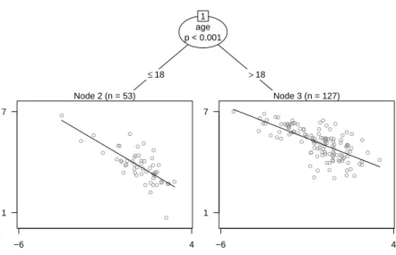
The resulting linear regression-based tree for the economic journals data is depicted in Figure 1 employing scatter plots with fitted regression lines in the leaves. In the fitting process, a global model for all observations is estimated (yielding a price elasticity of -0.53) and assessed by the parameter instability tests. A highly significant instability is found only with respect to age (with 1_{The median rather than the mean is used for two reasons: First, to account for the skewness of the performance}

distributions, and second due to the many bindings in the complexity measure for the model-based tree algorithms (MOB, GUIDE, M5’, LMT).

Achim Zeileis, Torsten Hothorn, Kurt Hornik 3 age p < 0.001 1 ≤18 >18 Node 2 (n = 53) ● ● ● ● ● ● ● ● ● ● ● ● ● ● ● ● ● ● ● ● ● ● ● ● ● ● ● ● ● ● ● ● ● ● ● ● ● ● ● ● ● ● ● ● ● ● ● ● ● ● ● ● ● −6 4 1 7 Node 3 (n = 127) ● ● ● ● ● ● ● ● ● ● ● ● ● ● ● ● ● ● ● ● ● ● ● ● ● ● ● ● ● ● ● ● ● ● ● ● ● ● ● ● ● ● ● ● ● ● ● ● ● ● ● ● ● _● ● ● ● ● ● ● ● ● ● ● ● ● ● ● ● ● ● ● _● ● ● ● ● ● ● ● ● ● ● ● ● ● ● ● ● ● ● ● ● ● ● ● ● ● ● ● ● ● ● ● ● ● ● ● ● ● ● ● ● ● ● ● ● ● ● ● ● ● ● ● ● ● ● −6 4 1 7

Figure 1: Linear-regression-based tree for the economic journals data. The plots in the leaves depict library subsriptions by price per citation (both in logs).

RMSE difference 0.00 0.02 0.04 0.06 0.08 0.10 RPart CTree M5' GUIDE ( ● ) ( ● ) ( ● ) ( ● ) Complexity difference 0 5 10 15 20 25 RPart CTree M5' GUIDE ( ● ) ( ● ) ( ● ) ( ● )

Figure 2: Performance comparison for economic journals data: prediction error is compared by RMSE differences, complexity by difference in number of estimated parameters (coefficients and split points).

a Bonferroni-adjustedpvalue ofp <0.001) which is subsequently used for splitting, leading to an optimal split at age 18. For the 53 young journals a much higher price elasticity of -0.6 is found than for the 127 older journals with a price elasticity of -0.4. No further parameter instabilities with respect to the partitioning variables can be detected (all p values are greater than 90%) and hence the algorithm stops. Table 1 reports the RMSE on the original data and the model complexity of 5 (2 timesk= 2 coefficients plus 2−1 splits).

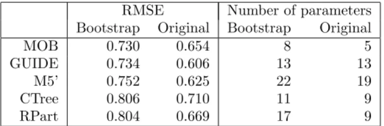
Table1and Figure2provide the results of the benchmark comparison on 250 bootstrap samples. The MOB trees have the lowest median RMSE and complexity, the simultaneous confidence inter-vals show that the differences compared to GUIDE are non-significant in both cases and significant compared to all other models. While the trees with constant fits are clearly outperformed with respect to RMSE, M5’ is still quite close in terms of RMSE but requires a substantially larger number of parameters to achieve this predictive performance.

RMSE Number of parameters Bootstrap Original Bootstrap Original

MOB 0.730 0.654 8 5

GUIDE 0.734 0.606 13 13

M5’ 0.752 0.625 22 19

CTree 0.806 0.710 11 9

RPart 0.804 0.669 17 9

Table 1: Performance comparison for economic journals data: prediction error is compared by median root mean squared error (RMSE) on 250 bootstrap samples and obvious RMSE on the original data set; complexity is compared by (median) number of estimated parameters.

3. Boston housing data

Since the analysis byBreiman and Friedman(1985), the Boston housing data are a popular and well-investigated empirical basis for illustrating non-linear regression methods both in machine learning and statistics (seeGama 2004;Samarov, Spokoiny, and Vial 2005, for two recent examples) and we follow these examples by segmenting a bivariate linear regression model for the house values. The data set provides n = 506 observations of the median value of owner-occupied homes in Boston (in USD 1000) along with 14 covariates including in particular the number of rooms per dwelling (rm) and the percentage of lower status of the population (lstat). A segment-wise linear relationship between the value and these two variables is very intuitive, whereas the shape of the influence of the remaining covariates is rather unclear and hence should be learned from the data. Therefore, a linear regression model for median value explained by (rm)2_{and log(lstat) withk= 3} regression coefficients is employed and partitioned with respect to all`= 11 remaining variables. As argued above, choosing appropriate transformations of the modeling variables is important to obtain a well-fitting model in each segment and we follow in our choice the recommendations of Breiman and Friedman(1985). The model is estimated by OLS, the instability is assessed using a Bonferroni-corrected significance level ofα= 0.05 and the nodes are split with a required minimal segment size ofi= 40.

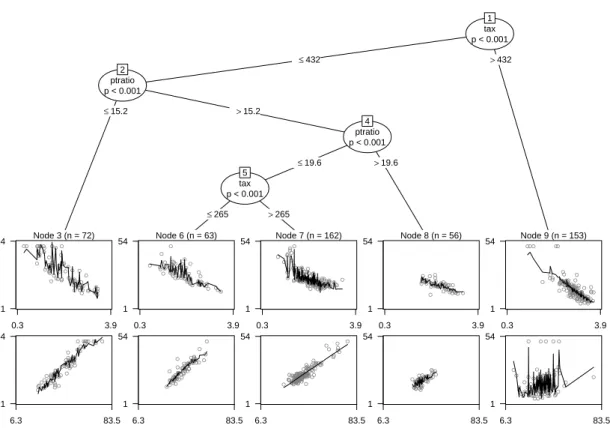
The resulting model-based tree is depicted in Figure3which shows partial scatter plots along with the fitted values in the terminal nodes. It can be seen that in the nodes 3, 6 and 7 the increase of value with the number of rooms dominates the picture (lower panel) whereas in node 9 the decrease with the lower status population percentage (upper panel) is more pronounced. Splits are performed in the variables tax (property-tax rate) and ptratio (pupil-teacher ratio). As reported in Table2, the model has 5·3 regression coefficients after estimating 5−1 splits, giving a total of 19 estimated parameters.

Achim Zeileis, Torsten Hothorn, Kurt Hornik 5 tax p < 0.001 1 ≤432 >432 ptratio p < 0.001 2 ≤15.2 >15.2 Node 3 (n = 72) ● ● ● ● ● ●● ● ● ● ● ● ●●●● ● ● ● ● ● ● ● ● ●● ● ●● ● ● ● ● ● ● ● ● ● ● ● ● ● ● ● ● ● ● ● ● ● ● ● ● ● ● ● ● ● ● ● ● ● ● ● ● ● ● ● ● ● ● ● 0.3 3.9 1 54 ● ● ●●● ● ● ● ●● ●●● ● ● ● ● ● ● ● ● ● ● ● ● ●● ● ● ● ●● ● ● ●● ● ● ● ● ● ● ● ● ● ● ● ● ● ● ●● ● ● ● ● ● ● ● ● ● ● ● ● ● ● ● ● ● ● ● ● 6.3 83.5 1 54 ptratio p < 0.001 4 ≤19.6 >19.6 tax p < 0.001 5 ≤265 >265 Node 6 (n = 63) ● ● ● ● ● ● ● ● ● ● ●●● ● ● ● ● ● ● ● ● ● ● ● ● ● ●● ● ● ● ● ● ● ●● ● ● ● ● ● ● ● ● ● ● ● ● ● ● ●● ● ● ● ● ● ● ● ● ● ● ● 0.3 3.9 1 54 ● ● ●● ●● ● ● ●● ● ●● ● ● ● ●● ● ● ● ● ●● ●● ●●● ●●● ● ● ● ● ● ● ●● ● ● ● ● ● ●● ● ● ●● ●● ● ● ● ● ● ● ● ● ● ● 6.3 83.5 1 54 Node 7 (n = 162) ● ● ● ● ● ● ● ● ● ● ● ● ● ●●● ● ●● ● ● ● ● ● ● ● ● ● ● ● ● ● ● ● ● ● ● ● ●● ●●● ●●●● ●● ● ● ● ● ● ● ● ●●● ● ● ● ● ● ● ●● ● ● ● ● ● ● ● ● ● ● ● ● ● ● ● ● ● ● ● ● ● ●● ●●● ● ● ● ● ● ● ● ● ● ● ● ●● ● ● ●●●● ● ● ● ● ● ● ● ● ● ● ● ● ●● ●●● ●● ● ● ● ● ● ● ● ● ● ● ● ● ● ● ● ● ● ● ● ● ● ● ● ●● ● ● ● ● ● ● 0.3 3.9 1 54 ● ● ● ●● ●● ●● ● ●●●●●●●●●● ● ● ● ● ● ● ● ● ●● ● ● ● ● ● ● ● ● ●●● ●●● ● ● ●●● ● ● ● ● ●● ●● ●● ●●●● ● ●●● ● ● ● ● ● ● ● ● ● ● ● ● ● ● ● ● ● ● ●● ● ●● ● ●● ● ● ● ● ● ● ●● ● ● ● ● ● ● ● ●●● ● ● ● ● ● ● ● ● ● ● ● ● ●●● ●●● ● ●●● ● ● ●● ● ● ● ● ● ●● ● ● ● ● ● ● ●●● ● ●● ● ● ●● ● ● 6.3 83.5 1 54 Node 8 (n = 56) ● ● ● ● ● ● ● ● ● ●● ● ● ●● ● ● ● ●●●● ● ●● ● ●● ● ● ● ●● ●●● ●●● ● ● ●●●●_●● ● ● ● ● ●● ● ● ● 0.3 3.9 1 54 ● ● ●● ● ● ● ● ● ● ●● ●●●● ● ●●● ● ● ● ● ● ● ●● ●● ● ● ● ● ● ● ●●●●●●●●●●● ● ● ●● ● ● ●● ● 6.3 83.5 1 54 Node 9 (n = 153) ● ● ● ● ● ● ● ● ● ● ● ● ● ● ●● ● ● ●● ● ● ● ● ● ● ● ● ●● ● ●● ●● ● ●●● ● ● ●●●●●●●● ● ● ● ● ●●●● ● ● ● ● ● ● ●● ● ● ● ● ● ● ●● ● ● ● ●● ●● ● ● ● ● ● ● ● ●●●●● ● ● ● ● ● ● ● ● ● ● ● ● ●● ● ●●●●●● ● ● ●● ● ● ● ● ● ● ● ●● ● ●●●●● ● ● ● ●●● ● ● ● ● ● ● ● ● ● ● ● ● ● ● ● 0.3 3.9 1 54 ● ● ● ● ● ●● ● ●● ●● ● ● ● ● ● ● ● ●● ● ● ● ● ● ● ● ● ●●● ● ● ● ●●●● ●●● ● ● ●●● ●●● ● ● ● ● ●●● ● ● ●●● ● ●● ● ● ● ● ● ● ● ● ● ● ●●● ●● ● ● ● ● ● ● ● ●●●● ● ● ● ● ● ● ● ● ● ● ● ● ● ●● ●●●● ●●●●●●●● ● ● ● ● ●● ● ●●●● ● ●●● ● ● ●● ● ● ● ●● ● ●● ●●● ● ● ● ● ● 6.3 83.5 1 54

Figure 3: Linear-regression-based tree for the Boston housing data. The plots in the leaves give partial scatter plots for log(lstat) (upper panel) and (rm)2_{(lower panel).}

RMSE difference 0.0 0.2 0.4 0.6 0.8 1.0 RPart CTree M5' GUIDE ( ● ) ( ● ) ( ● ) ( ● ) Complexity difference 0 100 200 300 RPart CTree M5' GUIDE (●) (●) (● ) (● )

Figure 4: Performance comparison for Boston housing data: prediction error is compared by RMSE differences, complexity by difference in number of estimated parameters.

perform significantly better on this data set than the other tree-based algorithms. The algorithm with the most comparable predictive performance, M5’, is here clearly inferior concerning its interpretability, requiring on average more than 12 times as many parameters.

RMSE Number of parameters Bootstrap Original Bootstrap Original

MOB 3.975 3.469 27 19

GUIDE 4.378 4.137 13 13

M5’ 4.058 2.482 348 321

CTree 4.607 3.428 43 37

RPart 4.838 4.193 17 13

Table 2: Performance comparison for Boston housing data: prediction error is compared by RMSE on 250 bootstrap samples and obvious RMSE on the original data set; complexity is compared by (median) number of estimated parameters.

4. Pima Indians diabetes data

Another popular data set for comparing new classifiers is the Pima Indians diabetes data which is— just as the Boston Housing data—available from the UCI machine learning repository (Newman, Hettich, Blake, and Merz 1998). The data comprises observations forn= 768 Pima Indian women of 8 prognostic variables and the outcome (positive/negative) of a diabetes test. It is rather clear that the diabetes diagnosis depends on the plasma glucose concentration such that using a logistic regression model for diabetes explained by glucose (corresponding tok= 2 parameters) is intuitive. This model is partitioned with respect to the remaining`= 7 variables, using a minimal segment size ofi= 40 and again a Bonferroni-corrected significance level ofα= 0.05.

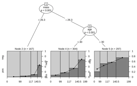
Figure5displays the resulting logistic regression-based tree. The data is first split at a body mass index of 26.3 (corresponding roughly to the lower quartile of this variable), those observations with a higher body mass index are partitioned into age groups below or above 30 years. The leaves of the tree visualize the data and the fitted logistic regression model using spinograms (Hofmann and Theus 2005) of diabetes by glucose (where the bins are chosen via the five point summary of glucose on the full data set). It can be seen that for women with a low body mass index the average risk of diabetes is low, but increases clearly with age (corresponding to an odds ratio of 1.060 per year). For the young women with a high body mass index, the average risk is higher and increases less quickly with respect to age (with an odds ratio of 1.048). Finally, the older women with a high body mass index have the highest average risk but with a lower odds ratio of only 1.024. The model uses 8 parameters (3·2 coefficients and 3−1 splits).

Misclassification Number of parameters Bootstrap Original Bootstrap Original

MOB 0.255 0.238 17 8 LMT 0.293 0.215 329 8 CTree 0.265 0.224 19 13 QUEST 0.265 0.250 23 3 J4.8 0.291 0.159 101 39 RPart 0.263 0.210 29 11

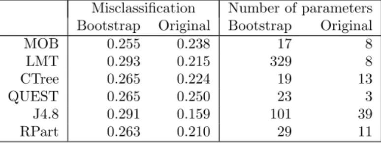
Table 3: Performance comparison for Pima Indians data: prediction error is compared by mis-classification rate on 250 bootstrap samples and obvious mismis-classification on the original data set; complexity is compared by (median) number of estimated parameters.

Achim Zeileis, Torsten Hothorn, Kurt Hornik 7 mass p < 0.001 1 ≤26.3 >26.3 Node 2 (n = 167) 0 99 117 140.5 pos neg 0 0.2 0.4 0.6 0.8 1 ● ● ● ● age p < 0.001 3 ≤30 >30 Node 4 (n = 304) 0 99 117 140.5 199 pos neg 0 0.2 0.4 0.6 0.8 1 ● ● ● ● Node 5 (n = 297) 0 99 117 140.5 199 pos neg 0 0.2 0.4 0.6 0.8 1 ● ● ● ●

Figure 5: Logistic-regression-based tree for the Pima Indians data. The spinograms in the leaves depict diabetes by plasma glucose concentration.

Misclassification difference 0.00 0.01 0.02 0.03 0.04 0.05 RPart J4.8 QUEST CTree LMT ( ● ) ( ● ) ( ● ) ( ● ) ( ● ) Complexity difference 0 50 100 150 200 250 300 350 RPart J4.8 QUEST CTree LMT ( )● ( )● ( )● ( )● ( )●

Figure 6: Performance comparison for Pima Indians data: prediction error is compared by mis-classification rate differences, complexity by difference in number of estimated parameters.

The results of the benchmark comparison in Table 3 and Figure 6 show that the MOB trees perform slightly (and significantly) better on this data set than the other tree-based algorithms included. In particular, it performs considerably better than the other model-based algorithm (LMT) both with respect to prediction and model complexity.

5. German breast cancer study

The same ideas used for recursive partitioning in (generalized) linear regression models can straight-forwardly be applied to other parametric regression models without further modification. Here, we apply the generic model-based recursive partitioning algorithm to a Weibull regression for mod-eling censored survival times. We follow the analysis of Schumacher, Holl¨ander, Schwarzer, and Sauerbrei(2001) andHothornet al.(2006a) who use constant fit survival trees to analyze survival times ofn= 686 women from positive node breast cancer in Germany. Along with the survival time (in years) and the censoring information, there are 8 covariates available as prognostic factors: number of positive lymph nodes, age, tumor size and grade, progesterone and estrogen receptor, and factors indicating menopausal status and whether the patient received a hormonal therapy. For explaining survival from positive node breast cancer in a regression model, the number of positive lymph nodes is chosen as explanatory variable with differing intercepts depending on whether a hormonal therapy was performed or not. Together with the scale parameter of the Weibull distribution, this gives a total of k = 4 parameters in the model, using the remaining

` = 6 prognostic variables for partitioning. The model is estimated by ML, the instability is assessed using a Bonferroni-corrected significance level ofα= 0.05 and the nodes are split with a required minimal segment size ofi= 40.

The resulting model-based tree is depicted in Figure 7 employing scatter plots for survival time by number of positive nodes in the leaves. Based on the ideas ofGentleman and Crowley(1991), circles with different shadings of gray (hollow and solid) are used for censored and uncensored observations, respectively. Fitted median survival times from the Weibull regression model are visualized by dashed and solid lines for patients with and with hormonal therapy. The data are

progrec p < 0.001 1 ≤24 >24 Node 2 (n = 299) ● ● ● ● ● ● ● ● ● ●●● ● ● ● ● ● ● ● ● ● ● ● ● ● ● ● ● ● ● ● ● ● ● ● ● ● ● ● ● ● ● ● ● ● ● ● ● ● ● ● ● ● ● ● ● ● ● ● ● ● ● ● ● ● ● ● ● ● ● ● ● ● ● ● ● ● ● ● ● ● ● ● ● ● ● ● ● ● ● ● ● ● ● ● ● ● ● ● ● ● ● ● ● ● ● ● ● ● ● ● ● ● ● ● ● ● ● ● ● ● ● ● ● ● ● ● ● ● ● ● ● ● ● ● ● ● ● ● ● ● ● ● ● ● ● ● ● ● ● ● ● ● ● ● ● ● ● ● ● ● ● ● ● ● ● ● ● ● ● ● ● ● ● ● ● ● ● ● ● ● ● ● ● ● ● ● ● ● ● ● ● ● ● ● ● ● ● ● ● ● ● ● ● ● ● ● ● ● ● ● ● ● ● ● ● ● ● ● ● ● ● ● ● ● ● ● ● ● ● ● ● ● ● ● ● ● ● ● ● ● ● ● ● ● ● ● ● ● ● ● ● ● ● ● ● ● ● ● ● ● ● ● ● ● ● ● ● ● ● ● ● ● ● ● ● ● ● ● ● ● ● ● ●●● ● ● ● ● ● ● ● ● ● ● ● ● ● 0 52 0 8 Node 3 (n = 387) ● ● ● ● ● ● ● ● ● ● ● ● ● ● ●●● ● ● ● ●● ● ● ● ● ● ● ● ● ● ● ● ● ● ● ● ● ● ● ● ● ● ● ● ● ● ● ● ● ● ● ● ● ● ● ● ● ● ● ● ● ● ● ● ● ● ● ● ● ● ● ● ● ● ● ● ● ● ● ● ● ● ● ● ● ● ● ● ● ● ● ● ● ● ● ● ● ● ● ● ● ● ● ● ● ● ● ● ● ● ● ● ● ● ● ● ● ● ● ● ● ● ● ● ● ● ● ● ● ● ● ● ● ● ● ● ● ● ● ● ● ● ● ● ● ● ● ● ● ● ● ● ● ● ● ● ● ● ● ● ● ● ● ● ● ● ● ● ● ● ● ● ● ● ● ● ● ● ● ● ● ● ● ● ● ● ● ● ● ● ● ● ● ● ● ● _● ● ● ● ● ● ● ● ● ● ● ● ●● ● ● ● ● ● ● ●● ● ● ● ● ● ●● ● ● ● ● ● ● ● ● ● ● ● ● ● ● ● ● ● ● ●● ● ● ● ● ● ● ● ● ● ● ● ● ● ● ● ● ● ● ● ● ● ● ● ● ● ● ● ● ● ● ● ● ●_● ● ● ● ● ● ● ● ● ● ● ● ● ● ● ● ● ● ● ● ● ● ● ● ● ● ● ● ● ● ● ● ● ● ● ● ● ● ● ● ● ● ● ● ● ● ● ● ● ● ● ● ● ●● ● ● ● ● ● ● ● ● ● ● ● ● ● ● ● ● ● ● ● ● ● ● ● ● ● ● ● ● ●● ● ● ● ● ● ● ● ● ● ● ●● ● ● ● ● ● ● ● ● ● ● ● 0 52 0 8

Figure 7: Weibull-regression-based tree for the German breast cancer study. The plots in the leaves depict censored (hollow) and uncensored (solid) survival time by number of positive lymph nodes along with fitted median survival for patients with (dashed line) and without (solid line) hormonal therapy.

Achim Zeileis, Torsten Hothorn, Kurt Hornik 9

partitioned once with respect to progesterone receptor splitting the observations into a group with marked influence of positive nodes and neglegible influence of hormonal therapy and a group with less pronounced influence of positive nodes but clear hormonal therapy effect. A fair amount of censored observations remains in both groups, no further significant instabilities can be detected (allpvalues are above 50%). The resulting model has 9 parameters (2·4 coefficients and 2−1 splits), yielding a log-likelihood of -809.9238.

For this survival regression problem, we refrain from conducting a benchmark comparison of per-formance as carried out in the previous section. The main reason for this is that it is not clear which predictive perfomance measure should be used in such a comparison: Whereas RMSE and misclassification are usually regarded to be acceptable (albeit not the only meaningful) perfor-mance measures for regression and classification tasks, the situation is not as well understood for censored regression models. Although various measures, such as the Brier score (Graf, Schmoor, Sauerbrei, and Schumacher 1999), are used in the literature their usefulness still remains a mat-ter of debate (Henderson 1995; Altman and Royston 2000; Schemper 2003). As resolving these discussions is beyond the scope of this paper, we content ourselves with the empirical analysis for this regression problem.

6. Conclusions

We illustrate how the generic algorithm for model-based recursive partitioning can be applied to different kinds of parametric models (linear regression, logistic regression, survival regression) yielding model-based trees that can be effectively visualized and intepreted. The benchmark comparisons show that the algorithm produces interpretable trees, competitive with previously suggested approaches for tree-based modeling.

References

Altman DG, Royston P (2000). “What Do We Mean by Validating a Prognostic Model?”Statistics in Medicine,19, 453–473.

Bergstrom TC (2001). “Free Labor for Costly Journals?” Journal of Economic Perspectives,15, 183–198.

Breiman L (2001). “Random Forests.”Machine Learning, 45(1), 5–32.

Breiman L, Friedman JH (1985). “Estimating Optimal Transformations for Multiple Regression and Correlation.”Journal of the American Statistical Association,80(391), 580–598.

Breiman L, Friedman JH, Olshen RA, Stone CJ (1984). Classification and Regression Trees. Wadsworth, California.

B¨uhlmann P, Yu B (2003). “Boosting withL2Loss: Regression and Classification.”Journal of the

American Statistical Association,98(462), 324–338.

Gama J (2004). “Functional Trees.”Machine Learning,55, 219–250.

Gentleman R, Crowley J (1991). “Graphical Methods for Censored Data.”Journal of the American Statistical Association,86, 678–683.

Graf E, Schmoor C, Sauerbrei W, Schumacher M (1999). “Assessment and comparison of prognostic classification schemes for survival data.”Statistics in Medicine,18(17-18), 2529–2545.

Henderson R (1995). “Problems and Prediction in Survival-Data Analysis.”Statistics in Medicine,

Hofmann H, Theus M (2005). “Interactive Graphics for Visualizing Conditional Distributions.” Unpublished Manuscript.

Hornik K, Zeileis A, Hothorn T, Buchta C (2006). RWeka: An RInterface to Weka. Rpackage version 0.2-2.

Hothorn T, Hornik K, Zeileis A (2006a). “Unbiased Recursive Partitioning: A Conditional In-ference Framework.” Journal of Computational and Graphical Statistics. Forthcoming, URL http://statmath.wu-wien.ac.at/~zeileis/papers/Hothorn+Hornik+Zeileis-2006.pdf. Hothorn T, Leisch F, Zeileis A, Hornik K (2005). “The Design and Analysis of Benchmark

Exper-iments.”Journal of Computational and Graphical Statistics,14(3), 675–699.

Hothorn T, Zeileis A, Hornik K (2006b). party: A Laboratory for Recursive Part(y)itioning. R

package version 0.8-3.

Landwehr N, Hall M, Frank E (2005). “Logistic Model Trees.”Machine Learning, 59, 161–205. Loh WY (2002). “Regression Trees With Unbiased Variable Selection and Interaction Detection.”

Statistica Sinica,12, 361–386.

Loh WY, Shih YS (1997). “Split Selection Methods for Classification Trees.”Statistica Sinica,7, 815–840.

Meyer D, Leisch F, Hornik K (2003). “The Support Vector Machine Under Test.”Neurocomputing,

55(1–2), 169–186.

Newman DJ, Hettich S, Blake CL, Merz C (1998). “UCI Repository of Machine Learning Databases.” URLhttp://www.ics.uci.edu/~mlearn/MLRepository.html.

Quinlan JR (1993).C4.5: Programs for Machine Learning. Morgan Kaufmann Publ., San Mateo, California.

Quinlan R (1992). “Learning with Continuous Classes.” In “Proceedings of the Australian Joint Conference on Artificial Intelligence,” pp. 343–348. World Scientific, Singapore.

R Development Core Team (2005). R: A Language and Environment for Statistical Computing.

R Foundation for Statistical Computing, Vienna, Austria. ISBN 3-900051-00-3, URL http: //www.R-project.org/.

Samarov A, Spokoiny V, Vial C (2005). “Component Indentification and Estimation in Nonlin-ear High-Dimension Regression Models by Structural Adaptation.” Journal of the American Statistical Association,100(470), 429–445.

Schemper M (2003). “Predictive Accuracy and Explained Variation.” Statistics in Medicine,22, 2299–2308.

Schumacher M, Holl¨ander N, Schwarzer G, Sauerbrei W (2001). “Prognostic Factor Studies.” In J Crowley (ed.), “Statistics in Clinical Oncology,” pp. 321–378. Marcel Dekker, New York. Stock JH, Watson MW (2003). Introduction to Econometrics. Addison Wesley.

Therneau TM, Atkinson EJ (1997). “An Introduction to Recursive Partitioning Using therpart

Routine.” Technical Report 61, Section of Biostatistics, Mayo Clinic, Rochester. URL http: //www.mayo.edu/hsr/techrpt/61.pdf.

Vapnik VN (1996). The Nature of Statistical Learning Theory. Springer, New York.

Wang Y, Witten IH (1997). “Induction of Model Trees for Predicting Continuous Classes.” In “Pro-ceedings of the European Conference on Machine Learning,” University of Economics, Faculty of Informatics and Statistics, Prague.

Achim Zeileis, Torsten Hothorn, Kurt Hornik 11

Witten IH, Frank E (2005). Data Mining: Practical Machine Learning Tools and Techniques. Morgan Kaufmann, San Francisco, 2nd edition.

Zeileis A, Hothorn T, Hornik K (2005). “Model-based Recursive Partitioning.” Report 19, De-partment of Statistics and Mathematics, Wirtschaftsuniversit¨at Wien, Research Report Series. URLhttp://epub.wu-wien.ac.at/.

A. Replication of results in

R

The followingRcode is sufficient for reproducing the empirical examples from Section??including data pre-processing, model fitting and visualization. The code for the benchmark comparisons is available upon request.

The results in this paper were obtained usingR2.2.1 and the packagesparty0.8–4,rpart3.1–27,

RWeka0.2–2,Ecdat0.1–4,ipred0.8–3,mlbench1.1–0,Weka3.4.7,QUEST1.9.1, andGUIDE2.1.

library("party")

data("Journals", package = "Ecdat")

journals <- Journals[, c("libprice", "society", "citestot")] journals$oclc <- log(Journals$oclc)

journals$citeprice <- log(Journals$libprice/Journals$citestot) journals$age <- 2000 - Journals$date1

journals$chars <- Journals$charpp*Journals$pages/10^6

mobJ <- mob(oclc ~ citeprice | society + citestot + age + chars + libprice, data = journals, model = linearModel, control = mob_control(minsplit = 10)) plot(mobJ)

data("BostonHousing", package = "mlbench") BostonHousing$lstat <- log(BostonHousing$lstat) BostonHousing$rm <- BostonHousing$rm^2

BostonHousing$chas <- factor(BostonHousing$chas)

BostonHousing$rad <- factor(BostonHousing$rad, ordered = TRUE)

mobBH <- mob(medv ~ lstat + rm | zn + indus + chas + nox + age + dis + rad + tax + crim + b + ptratio, data = BostonHousing,

control = mob_control(minsplit = 40), model = linearModel) plot(mobBH)

data("PimaIndiansDiabetes", package = "mlbench")

mobPID <- mob(diabetes ~ glucose | pregnant + pressure + triceps + insulin + mass + pedigree + age, data = PimaIndiansDiabetes, model = glinearModel, control = mob_control(minsplit = 40), family = binomial())

plot(mobPID)

data("GBSG2", package = "ipred") nloglik <- function(x) -logLik(x) GBSG2$time <- GBSG2$time/365

mobGBSG2 <- mob(Surv(time, cens) ~ horTh + pnodes | progrec + menostat + estrec + menostat + age + tsize + tgrade, data = GBSG2, model = survReg, control = mob_control(objfun = nloglik, minsplit = 40))