Contrastive Representation Learning:
A Framework and Review
PHUC H. LE-KHAC 1, GRAHAM HEALY 2, AND ALAN F. SMEATON 2,3, (Fellow, IEEE)
1ML-Labs, Dublin City University, Dublin 9, D09 Ireland 2School of Computing, Dublin City University, Dublin 9, D09 Ireland 3Insight Centre for Data Analytics, Dublin City University, Dublin 9, D09 Ireland Corresponding author: Phuc H. Le-Khac ([email protected])
This work was supported in part by the Science Foundation Ireland through the Science Foundation Ireland (SFI) Centre for Research Training in Machine Learning (18/CRT/6183) and in part by the Insight Centre for Data Analytics (SFI/12/RC/2289_P2).
ABSTRACT Contrastive Learning has recently received interest due to its success in self-supervised representation learning in the computer vision domain. However, the origins of Contrastive Learning date as far back as the 1990s and its development has spanned across many fields and domains including Metric Learning and natural language processing. In this paper, we provide a comprehensive literature review and we propose a general Contrastive Representation Learning framework that simplifies and unifies many different contrastive learning methods. We also provide a taxonomy for each of the components of contrastive learning in order to summarise it and distinguish it from other forms of machine learning. We then discuss the inductive biases which are present in any contrastive learning system and we analyse our framework under different views from various sub-fields of Machine Learning. Examples of how contrastive learning has been applied in computer vision, natural language processing, audio processing, and others, as well as in Reinforcement Learning are also presented. Finally, we discuss the challenges and some of the most promising future research directions ahead.
INDEX TERMS Contrastive learning, representation learning, self-supervised learning, unsupervised learning, deep learning, machine learning.
I. INTRODUCTION
The performance of a machine learning system is directly determined by the choice and quality of the data representa-tion, or features, in the data used to train it. While it is obvious that some criteria for usefulness depend on the task, it is also universally assumed that there are sets of features that are representative of a dataset and that are generally useful as input for many kinds of downstream classifier or predictor. Focusing explicitly on learning representation in some cases can be beneficial, for example, when a labelled dataset for a task is small and we want to leverage a larger unlabelled dataset to improve the performance of a learning system.
Representation learningrefers to the process of learning a parametric mapping from the raw input data domain to a feature vector or tensor, in the hope of capturing and extracting more abstract and useful concepts that can improve performance on a range of downstream tasks. Often the input
The associate editor coordinating the review of this manuscript and approving it for publication was Shagufta Henna.
domain has a high dimensional space (images, video, sound, text) and the encoded representations reside in a manifold of a much lower dimensionality. While all dimensional-ity reductionmethods convert high-dimensional inputs to a lower-dimensional representation, some of these methods do not learn a mapping that meaningfully generalises on new data samples, and that is what representation learning does.
In the early day of Machine Learning (ML), much effort was spent on designing data transformation and pre-processing pipelines, and learning was only used to make a shallow decision based on extracted features. One of the key ingredients in the success of deep learning is the ability to learn and extract through deep layers some use-ful features from data. The increase in available computa-tion and labelled datasets has enabled the paradigm shift from using hand-designed feature extractors to learned fea-ture extractors. As a result, the focus in research also shifted from feature-engineering to architecture-engineering. Research into deep learning architectures has exploded in recent years and has matured into a few core principles and
building blocks e.g convolution layer for local data, recurrent layer for sequential data, and attention layer for set data.
As a goal, the task of explicitly learning a good sentation in comparison to implicitly learning a good repre-sentation to optimise performance for a task, can be tricky. Firstly, it is not entirely clear what makes a good repre-sentation. Based on the analysis by Bengio, Courville, and Vincent [9], a good representation has the properties of local smoothness of input and representation, is temporally and spatially coherentin a sequence of observations, has multi-ple, hierarchically-organised explanatory factors which are sharedacross tasks, hassimple dependenciesamong factors and issparselyactivated for a specific input.
From these criteria the field of Representation Learning, especially in the Deep Learning circle, has itself developed a number of core principals used to learn a good representation and these are:
• Distributed: Representations that are expressive and can represent an exponential amount of configuration for their size. This is in contrast with other types of representations such as one-hot encoding, learned by many clustering algorithms;
• Abstraction and Invariant: Good representations can capture more abstract concepts that are invariant to small and local changes in input data;
• Disentangled representation: While a good representa-tion should capture as many factors and discard as little data as possible, each factor should be asdisentangledas possible. Aside from promoting feature re-use in learn-ing systems, it can also be beneficial for other purposes such as explainability.
While distributed representation and abstraction can be achieved to some degree through deep network architec-tures, invariant and disentangled representations are harder to achieve and are usually implicitly learned with the task. A family of methods collectively calledContrastive Learning offers a simple method to encode these properties within a learned representation.
In this paper, we formulate and discuss a Contrastive Representation Learning (CRL) framework, which poten-tially represents another paradigm shift from architecture-engineeringtodata-engineering.
Even though contrastive learning has become prominent in recent years due to the success of large pre-trained mod-els in the fields ofnatural language processing(NLP) and computer vision(CV), the seminal idea dates back at least to the 1990s [8], [11]. Furthermore, the development into its current form has spanned over multiple sub-fields and appli-cation domains, which can make understanding it challenging although the core intuition behind its operation has remained unchanged. In addition, due to the recent successes of con-trastive learning in instance discrimination self-supervised learning, it is often incorrectly regarded merely as another self-supervised learning technique, which does not do justice to the generality of contrastive methods.
With the recent surge in interest in Contrastive Learning methods, there is much published work associated with con-trastive learning but without a proper framework to analyse this work, it can be hard to understand the novelties and trade-offs of new methods. This paper proposes a simple yet powerful framework that can be used to categorise and explain in simple terms, the progress in this sub-field, rang-ing from supervised to self-supervised methods, in multiple application and input domains including images, videos, text and audio and their combinations. To the best of our knowl-edge, this is the first paper to survey the specific history and recent development of the contrastive approach in a wide range of domains.
In summary, these are the contributions of this paper: • We propose a simple framework to understand and
explain the workings of contrastive representation learning;
• We provide a comprehensive survey of its history and development, and a taxonomy for each of the frame-work components as well as a summary of conceptual advancements spanning over many sub-fields;
• We study and make connections between the contrastive approach and various other methods;
• We present the application of contrastive learning in various application domains and tasks;
• We analyse the current limits and discuss future research directions.
The rest of the paper is organised as follows. In the next section, we present an introduction and an overview of what contrastive learning is with an emphasis on contrastive learn-ing of representations. That is followed by a taxonomy of how we see contrastive learning starting with a formal framework description and then presenting various ways in which the field can be divided based on similarity, encoders, transform heads and loss functions. SectionIVthen presents a variety of data domains and problem topics to which contrastive learning has been applied, covering applications in language, vision, audio, graph-structured data, multi-modal data and other areas. We then present a discussion of several topical issues with an emphasis on future outlook, and a concluding section completes the paper.
II. WHAT IS CONTRASTIVE LEARNING ?
We now present an overview of different representation learn-ing approaches and an intuitive introduction to contrastive learning with a concrete example of theInstance Discrimina-tiontask in learning self-supervised visual representations.
A. REPRESENTATION LEARNING
1) GENERATIVE AND DISCRIMINATIVE MODELS
In the machine learning literature, approaches to learning representations of data are often divided into two main cat-egories: generative or discriminative modelling. The process of extracting representations, or inferring latent variables from a probabilistic view of a dataset, is often called inference. While both approaches assume that a good
representation will capture the underlying factors that explain variations in the datax, they differ in the process of learning these representations. Generative approaches learn represen-tations by modelling the data distributionp(x), for example: all the pixels in an image. It is based on the assumption that a good modelp(x) that can generate realistic data samples, must also in turn capture the underlying structure related to the explanatory variables y. Evaluating the conditional distributionp(y|x) for some discriminative tasks on variable ycan then be obtained by using Bayes’ rule.
Discriminative approaches to learning representations on the other hand learn a representation by directly modelling the conditional distributionp(y|x) with a parametrised model that takes as input the data sample x and outputs the label variabley. Discriminative modeling consists of an inference step that infers the values of the latent variables p(v|x), and then directly makes downstream decisions from those inferred variablesp(y|v).
Discriminative models have some advantages when com-pared to generative models. Modelling the distribution for the set of datax ∈ X is computationally expensive and is not necessary in order to extract representations. If the goal is only to learn a mapping to a lower dimension represen-tation, the generation process in a generative model can be considered wasteful. In addition, the task of learning a good decoder/generator can be entangled with the task of learning a good feature encoder. The objective functions of generative models are also more expensive to evaluate and harder to design since they usually operate in the input space.
2) SUPERVISED AND UNSUPERVISED LEARNING
Until recently, the most successful applications of deep learn-ing belonged to the class of supervised learnlearn-ing methods, where a representation is directly learned by mapping from the input to a human-generated label i.e. in training data pairs (x,y), to optimise an objective function. Earlier paradigms involving pre-training layer-wise unsupervised models pro-vided little or no benefit in an end-to-end supervised setting. As the performance of deep learning can scale upwards with the amount of data and the model size [55], the need for labelled data has been identified as an impeding factor in scal-ing deep networks. Labellscal-ing data has its own set of disadvan-tages such as being time-consuming and expensive, as well as carrying privacy concerns when labelling is out-sourced to a third-party, for example in medical data, as well as potentially injecting annotators’ biases through the labelling process.
Previously, most unsupervised representation learning methods belong to the class of generative models [32], [58]. While generative models provide a general objective to learn a low-dimensional representation, they are computationally expensive and are also limited by the ability to model the dependencies between input dimensions.
Until recently, most discriminative approaches to learning representations are a type of supervised learning. Some newer works under the term ‘‘self-supervised’’ learning aim to learn useful representations without labels using discriminative
modelling approaches. These methods have shown great suc-cess when used for transfer learning, surpassing supervised pre-trained models in multiple downstream tasks, in both computer vision and natural language processing applica-tions. Since a self-supervised discriminative model does not have labels corresponding to the inputs like its supervised counterparts, the success of self-supervised methods comes from the elegant design of the pretext tasks to generate a pseudo-labelyˆfrom part of the input data itself [26], [118].
Among the most successful of the recent self-supervised approaches to learning visual representations, a subset of these termed ‘‘contrastive’’ learning methods have achieved the most success.
3) OBJECTIVE AND EVALUATION OF REPRESENTATIONS As distinct from supervised tasks where we can optimise for the goal directly, there is no straightforward objective for learning good representation that we can measure. A good representation can be useful to improve the performance of downstream tasks, but this objective requires prior knowledge of the task we ultimately want to optimise for. In other cases, where a lot of tasks share the same input data (e.g image classification / detection / segmentation), we can argue that a good representation captures the inherent properties of the underlying data and should be shared across those tasks. However the representations for these tasks can sometimes be in conflict, especially when the capacity of the model is not enough, and there is a trade-off between performance in one task and generalisability across multiple tasks.
In some other cases where a representation is learned through a proxy task, the performance of the proxy task can also be a proxy performance measure for the representation, such as a generative model measuring the reconstruction error, fidelity and diversity of generated samples. This is the case for contrastive representation learning, where the quality of the representation is approximated by how well the representation separates similar and dissimilar samples.
Moreover, sometimes learning a good representation can be an effective way to study the inherent characteristics of the data itself, without the need to perform any particular task.
B. CONTRASTIVE REPRESENTATION LEARNING
Intuitively, contrastive representation learning can be consid-ered as learning by comparing. Unlike a discriminative model that learns a mapping to some (pseudo-)labels and a gener-ative model that reconstructs input samples, in contrastive learning a representation is learned by comparing among the input samples. Instead of learning a signal from individual data samples one at a time, contrastive learning learns by comparingamong different samples. The comparison can be performed between positive pairs of ‘‘similar’’ inputs and negative pairs of ‘‘dissimilar’’ inputs.
Unlike supervised methods where a human annotation yis needed for every input sample x, contrastive learning approaches only need to define the similarity distribution in order to sample a positive inputx+ ∼ p+(·|x), and a data
distribution for a negative inputx− ∼p−(·|x), with respect to an input samplex. The goal of contrastive learning is very simple: the representation of ‘‘similar’’ samples should be mapped close together, while that of ‘‘dissimilar’’ samples should be further away in the embedding space. Thus by con-trasting between samples of positive and samples of negative pairs, representations of positive pairs will be pulled together while representations of negative pairs are pushed far apart.
In the self-supervised setting, instead of deriving a pseudo-label from the pretext task, contrastive learning meth-ods learn a discriminative model on multiple input pairs, according to some notion of similarity. Similar to other self-supervised pretext tasks, this definition of similarity can be defined from the data itself, and thus can overcome a limitation encountered in supervised learning settings where only a finite number of label pairs are available from the data. While some self-supervised methods need to modify the model architecture during learning (such as in [118]), contrastive methods are much simpler where no modification to the model architecture is needed between training and fine-tuning to other tasks.
If additional labels are provided, these can also be inte-grated into the definition of similarity and dissimilarity of the contrastive framework as well. By defining the similarity and dissimilarity distribution on the dataset level instead of individual data samples, contrastive methods alleviate the need for a labelled dataset while providing a mechanism to specify the desired invariant / covariant properties of the learned mapping. Thus contrastive learning methods provide a simple yet powerful approach to learning representations in a discriminative manner in both supervised or self-supervised setups.
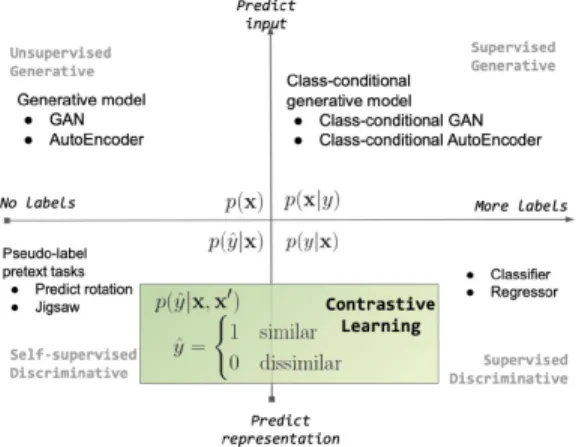
FIGURE 1. Contrastive learning in the Generative-Discriminative and Supervised-Unsupervised spectrum. Contrastive methods belong to the group of discriminative models that predict a pseudo-label ofsimilarity ordissimilaritygiven a pair of inputs.
Figure1illustrates the family of contrastive methods along generative-discriminative and supervised-unsupervised axes.
C. EXAMPLE: INSTANCE DISCRIMINATION
Along the lines of an exemplar-based classification task [26], which treats each image as its own class, Instance Dis-crimination [110] is a popular self-supervised method to
learn a visual representation and has succeeded in learn-ing useful representations that achieve state-of-the-art results in transfer learning for some downstream computer vision tasks [43], [69]. Based on the simple formulation proposed in SimCLR [16], in this section we will describe the Instance Discrimination task as a simple form of contrastive learning, as illustrated in Figure2.
FIGURE 2. Contrastive learning in the Instance Discrimination pretext task for self-supervised visual representation learning. A positive pair is created from two randomly augmented views of the same image, while negative pairs are created from views of two different images. All views are encoded by the a shared encoder and projection heads before the representations are evaluated by the contrastive loss function.
The image-based instance discrimination pretext task learns a representation by maximising agreement of the encoded features (embeddings) between two differently aug-mented views of the same images, while simultaneously minimising the agreement between views generated from different images. To avoid the model maximising agreement through low-level visual cues, views from the same images are generated through a series of strong image augmentation methods.
• Let T be the set of image transformation operations wheret,t0∼T are two different transformation opera-tors independently sampled fromT. These transforma-tions could be randomcroppingandresizing,blur,color distortionorperspective distortion, etc. A (xq,xk) pair of query and key views is positive when these two views are created by applying different transformations on the same imagex:xq=t(x) andxk =t0(x), and is negative otherwise.
• A feature encoder e(·) then extracts the feature vec-tors from all the augmented data samples v = e(x). There is no restriction on the choice of the encoder but a ResNet [42] model is usually used for image data because of its simplicity. The representationv ∈ Rd in this case is the output of the average pooling layer of Resnet.
• Each representationvis then fed into aprojection head h(·) comprised of a small multi-layer perceptron (MLP) to obtain a metric embeddingz=h(v), wherez∈ Rd0
with d0 < d is in a lower dimensional space than the representation v. This projection head can be as simple as a one-layer MLP using a non-linear activation function. All the vectors are then normalised to be unit vectors.
• A batch of these metric embedding pairs{(zi,z0i)}, with (zi,z0i) represents the metric embeddings from two aug-mented versions (xq,xk) of the same image, are then fed into thecontrastive lossfunction which encourages the distance in the metric embedding of the same pair to be small, and the distances of embeddings from differ-ent pairs to be large. The non-parametric classification loss [110] and its variants, such as InfoNCE [77] and NT-Xent [16] is a popular choice for the contrastive loss function, which for the i-th pair has the general form: Li= −log exp(z>i z0i/τ) PK j=0exp(zi·z0j)/τ) (1)
wherez>z0is the dot product between two vectors and τ is a temperature hyper-parameter that controls the sensitivity of the product. The sum in the denominator is computed over one positive andK negative pairs in the same minibatch. Intuitively, this can be understood as a non-parametric version of (K +1)-way softmax classification [110] ofzito the correspondingz0i. In order to minimise the InfoNCE loss function in Eq. (1), the dot product in the numerator measuring the similar-ity of representation from the same pair is maximised, while the similarity of all negative pairs in the denominator, is minimised.
When the contrastive training phase is done, the projection head is discarded and the encoder is used as the feature extractor for transfer learning. By combining the predictor or classifier with the representation output of the encoder, they can be fine-tuned on a new task on a target dataset.
Contrastive methods in the instance discrimination task set out to learn a representation that can separate between different instances, while ignoring the meaningless variances introduced by image data augmentation. Because contrastive learning directly maximises similarity between representa-tions of positive similar pairs and minimises that of nega-tive pairs, how those pairs are generated directly determines the invariant properties in the learned representation. The most important components for the success of contrastive pre-training on ImageNet [23] is data augmentation methods. As analysed in SimCLR [16], many contrastive methods per-form very poorly without proper augmentations (i.e random crop and color distortion) even for the same set of architec-tures and losses.
The dataset, data transformations and instance-wise simi-larity definition combined together in the contrastive learning framework provide a scalable and accessible approach to specifying invariant and covariant properties in the learned representation.
III. A TAXONOMY FOR CONTRASTIVE LEARNING
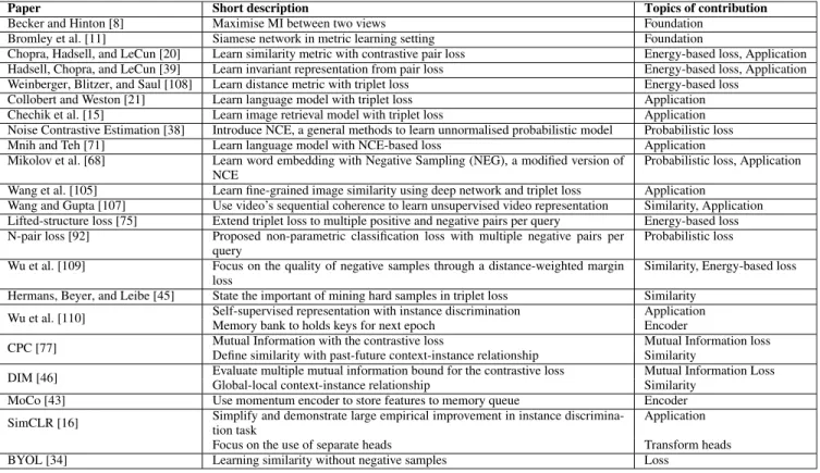
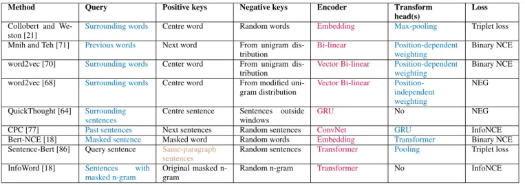
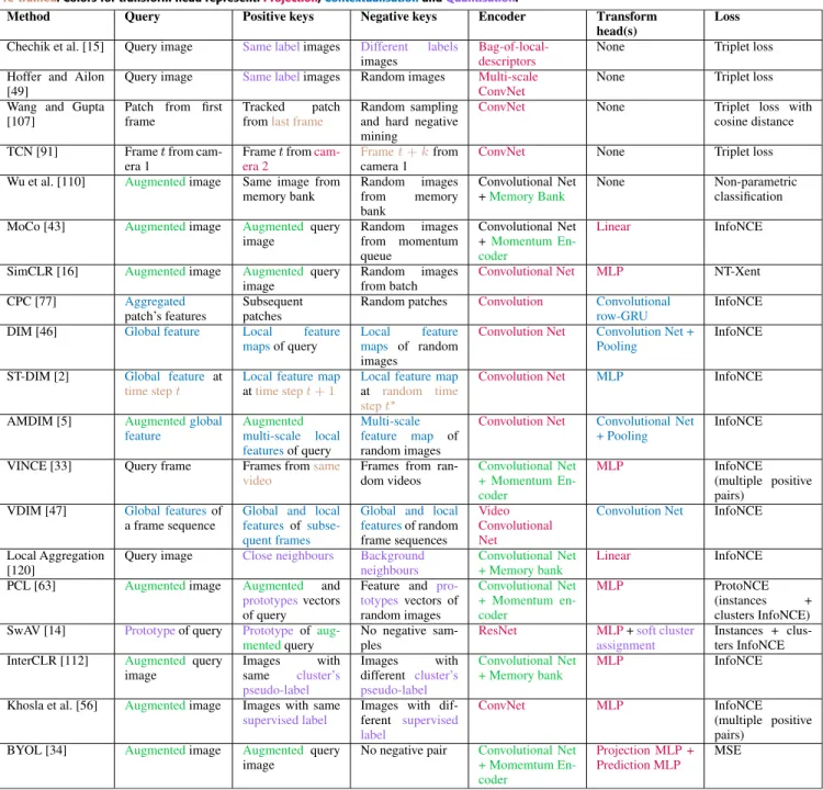
Before we present our taxonomy for contrastive learning methods, we first formally describe the contrastive represen-tation learning (CRL) framework in SectionIII-A. In partic-ular, the CRL is a general framework that can be used to succinctly describe a variety of contrastive learning meth-ods ranging from self-supervised to supervised and covering images, videos, audio, text and more. We use this frame-work to introduce a comprehensive taxonomy for the com-ponents of contrastive methods in SectionsIII-B,III-C,III-D andIII-E.
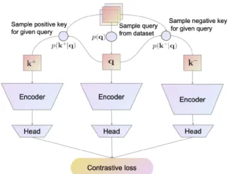
FIGURE 3. Overview of the Contrastive Representation Learning framework. Its components are: a similarity and dissimilarity distribution to sample positive and negative keys for a query, one or more encoders and transform heads for each data modality and a contrastive loss function evaluate a batch of positive and negative pairs.
A. THE CONTRASTIVE REPRESENTATION LEARNING FRAMEWORK
The general CRL framework, illustrated in Fig.3builds on top of the work of Chenet al.[16], which describes a simple contrastive self-supervised framework to learn visual repre-sentations in the context of an Instance Discrimination task (see SectionII-C). As distinct from [16], we generalise this framework beyond the image Instance Discrimination task to cover learning representations in a variety of data domains (images, video, audio and text), learning setups (supervised, self-supervised or knowledge distillation) and ways to define the concept of similarity. Specific choices of the similarity distribution, encoders and heads as well as contrastive loss functions allows the CRL framework to encompass arbitrary contrastive learning methods. More importantly, it enables a clear understanding of most of the contemporary work and sheds light on the limitations and the promising directions ahead.
In the following and throughout the rest of the paper, we adopt the metaphor of query and key similar to [43], by considering the problem of similarity matching as a form of dictionary look-up.
We will use the symbols qand k to represent thequery andkey for either the input sample x, the representation v or the metric embeddingzdepending on context. When we need to be specific, the corresponding symbolsx,v,zwith superscript·q,·kfor query and key will be used.
Definition 1 (Query, Key): Queryand key refer to a par-ticular view of an input samplex ∈ X. Together they form a positive or negative pair (q,k) depending on whether the query and key are considered similar or not.
In the Instance Discrimination task, query and key views are a randomly transformed version of an imaget(x) in the data setX.
Definition 2 (Similarity Distribution): Asimilarity distri-bution p+(q,k+) is a joint distribution over a pair of input samples that formalises the notion of similarity (and dis-similarity) in the contrastive learning task. Distinct from other machine learning methods where the data distribution is defined over a single input sample p(x), the similarity required by contrastive methods takes input from the joint distributions of pairs of samplesp(q,k).
A key is considered positive k+ for a query q if it is sampled from this similarity distribution and is considered negativek−if it is sampled from the dissimilarity distribution p−(q,k−). In some tasks, the dissimilar data distribution may not be explicitly defined but implicitly given as the distribution of any pair that is not sampled from the similarity distribution.
Similar to other representation learning problems, the focus of contrastive learning is in learning from a high-dimensional input space X, which depends on the domain and can be a tensor representing audios, images, videos or texts.
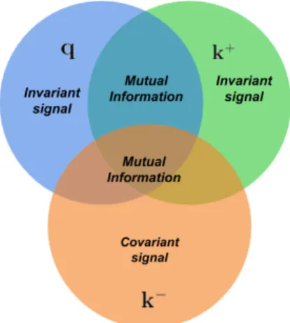
Combining the data distribution p(x), the definition of similarity p+(q,k) and dissimilarity p−(q,k−), different properties of the learned representation can be specified, as illustrated in Figure4.
In practice, queries and keys are not necessarily sampled jointly but the query can be sampled first from the data dis-tributionq∼p(x) where then the corresponding positive and negative keys are sampled from the conditional distributions k+∼p+(·|q) andk−∼p−(·|q).
In the Instance Discrimination task, the similarity distribu-tion is defined over any pair that are transformed from the same input samplesq,k∼p+(·,·) ifq=t(x) andk=t0(x) for 2 different random transformationstandt0∈T.
Definition 3 (Model): We refer to the combination of all modules with parameters in a contrastive learning method as themodelf(x;θ):X →R|Z|and its parameters collectively asθ.
The model can be decomposed further into a base encoder and a transform head.
Definition 4 (Encoder): The features encoder e(x;θe) : X → V with parameters θe learns a mapping from the input views x ∈ X to a representation vector v ∈ Rd. This network (when trained via contrastive learning) can be used to generate features (or inputs) to leverage the learned
FIGURE 4. An intuitive diagram represents the learning signal captured by the contrastive loss through the query, positive and negative keys. Contrastive methods allow the desired invariances to be specified through the similarity and dissimilarity distributions. Each circle represents the information signal contained in each view. The signal that is not mutual between query and positive keys are invariant features, since their representations are made as similar as possible. The signal that is not mutual between the negative key and the query or positive keys are covariant features, since these representations must be able to distinguish between those to minimise similarity to the negative key.
representations in other tasks (e.g. as input when learning another model for an image classification task), or to have layers stacked on top (e.g. fully connected, softmax) where the network can be fine-tuned to the new task.
Definition 5 (Transform Head): Transform heads h(v; θh):V →Zparameterised byθh, are modules that transform the feature embedding v ∈ V into a metric embedding z∈Rd0.
Depending on the specific application, the transform heads can be used to aggregate information from multi-ple representation vectors or used to project it down to a lower-dimensional space before the contrastive loss.
Definition 6 (Contrastive Loss): A contrastive loss func-tion operates on a set of metric embedding pairs{(z,z+), (z,z−)}of the query, positive and negative keys. It measures the similarity (or distance) between the embeddings and enforces constraints such that the similarity of positive pairs are high and the similarity of negative pairs are low. To attain small distances between the embeddings of positive pairs in the metric space, representations will becomeinvariant to irrelevant differences in the input space of positive pairs, while simultaneously learning thecovariant representation between negative pairs to explain for the large distance in the metric space.
B. A TAXONOMY OF SIMILARITY
Contrastive Learning revolves around learning a mapping from different views of the samescene, or contextinto the same region of a representation space, which is formalised through the similarity distribution. The key to an effective contrastive learning task is to design the similarity distribu-tion such that positive pairs are very different in the input
space yet semantically related, and a dissimilarity distribu-tion such that negative pairs are similar in the input space but semantically different. Despite the recent popularity of self-supervised contrastive learning, contrastive learning in general is agnostic to the supervised / unsupervised paradigm. Depending on whether any human labelsyare used in defin-ing those joint distribution (e.g.k∼p(·|q,y), the method then becomes a supervised or self-supervised contrastive learning task.
Depending on the end goals there can be many notions of similarity and dissimilarity, which is a strong point of contrastive methods, but it also makes it difficult to provide a taxonomy that captures all these variations. However, there are some general principles that are usually the underlying assumptions behind how similarity and dissimilarity is con-structed, which we now examine.
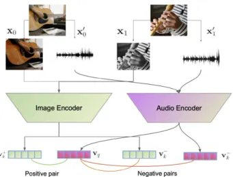
FIGURE 5. Illustration of learning similarity between multiple modalities. Each modality has an encoder and the representations extracted by different encoders are contrasted with each other to learn a joint embedding space.
1) MULTISENSORY SIGNALS
One direct approach to have multiple views of the same context is to record the information with multiple sensors. These sensors can be of the same modality (e.g. two cam-eras recording the same scene from different angles), or of different modalities (e.g. audio and image from a video), as illustrated in Fig. 5. Using the natural correspondence between different sensors, the model can learn to be invariant to the low-level details in each sensor input and focus on representing the shared context between them.
Contrastive methods have been used to learn cross-modal representations of visual and textual data in [50], [96]. In the Time-Contrastive Network [91], a visual representation is learned by pulling the representation of two simultaneous views fromdifferent camerasof the same scene, while push-ing apartframes taken from far away in time but from the same video. This leads to a representation space that is invariant to viewpoints while being sensitive to changes in time.
2) DATA TRANSFORMATION
If synchronous data from multiple sensors is not available (e.g. a single-modality dataset like ImageNet), the most sim-ple yet effective approach to generating different views of the same scene is to use a hand-crafted transformation function operating on the input data domain. Designing and imple-menting such semantic-preserving transformations requires prior knowledge, but this knowledge is defined once for the entire dataset or data collection pipeline, and can be dynami-cally applied to individual samples at run time.
FIGURE 6. Illustration of some common image augmentation methods. Different views from a random set of augmentations of the same images are usually considered positive pairs.
For visual data, image augmentation methods such as lighting or color distortion,cropping and padding,adding noise and blur,rotation and perspective transform etc. are efficient methods to transform pixels while preserving the semantic meaning of an image’s content such as its class labels. An example of these data transformations techniques on image can be seen in Fig.6. Destroying low-level visual cues by image augmentation forces the contrastive method to learn a representation invariant to those changes in the inputs. These techniques have been widely used in supervised learning to learn invariant features and to increase the robust-ness of the resulting models. The recent wave of instance dis-crimination contrastive methods have demonstrated that the same representation can be learned from these augmentation techniques without the need for a class label [16], [43], [69], [110], [117].
For natural language text data, Fanget al.[29] transform a sentence using a back-translation method to create a slightly different sentence that has the same semantic meaning as the original one to form a positive pair. Back-translation uses two machine translation models to translate a sentence into a target language and back to the source language. The random-ness from the two translation models will yield a sentence in the source language that is slightly different from the original sentence.
For program code data, ContraCode [51] uses various source-to-source transformation methods from the com-piler literature such as variable renaming, identifier man-gling,reformatting, beautification, compression,dead-code
insertion / elimination, etc. to construct semantically similar code snippets that share the same functionality. Learning to map these textually different but functionally equivalent programs to the same feature vector allows the model to learn a function representation space that is predictive of equivalent programs.
For audio data, some augmentation methods such as warp-ing,frequency and temporal maskingin the Mel spectrogram format could be used to create different version of the same audio data, as in [73].
3) CONTEXT-INSTANCE RELATIONSHIP
Another approach to extracting similar views of the same scene is by exploiting the context-instance relationship from a sample representation. Generally, we want to learn a rep-resentation that captures the entire context, i.e the global information about a scene. That context can usually be decomposed further into parts, each containing a subset of the scene’s information that is local to each subset.
Explicitly constraining the representation of the parts (local features) to be similar to the representation of the whole (global features), while being different from the rep-resentation of other views is a clever approach to defining similarity. Contrasting between the representation of local features versus global features can encourage the model to learn important features that present in the local views, while ignoring noise features which occur only in those local inputs. Representation from local features is thus encouraged to capture meaningful information relevant to the whole context, while global features are encouraged to capture as much detail from the local instances as possible.
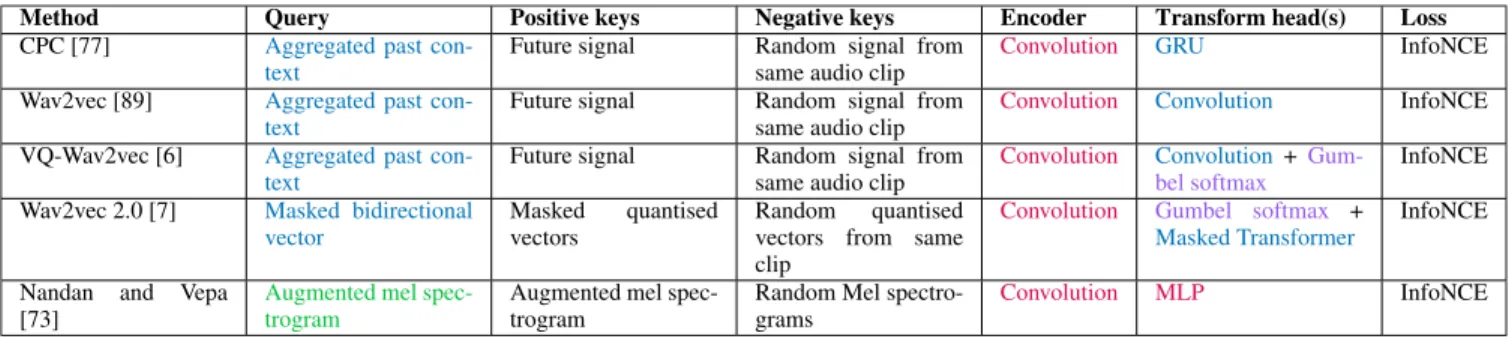
FIGURE 7. Illustration of extracting query and keys using the context-instance relationship. Ina), the context is a global summary vector of the entire image, while the instances are the local features in the set of intermediate feature maps. Inb), the past context is aggregated with a RNN contextualisation head and the instance are representations of future time steps.
Figure7a describes the approach taken in Deep InfoMax (DIM) [46], where an image is encoded into a global feature vector and also into a feature map corresponding to spatial patches of pixels in the original image. The global feature
and local features in the feature map of the same images then form positive pairs, while global features with local features from other images are considered negative pairs.
Global features can also be constructed from videos in the temporal dimension, as in Fig.7b. In Contrastive Predictive Coding (CPC) [77], context features are constructed as a summary of past input segments, and then contrasted with local features from a future time step. Contrastive learning to predict the correct future from the past context in this way can be thought of as an instantiation of the predictive coding theory.
4) SEQUENTIAL COHERENCE AND CONSISTENCY
In addition to the context-instance feature relationship, exploiting the spatial or temporal coherence and consistency in a sequence of observations is another approach to defining similarity in contrastive learning. This method works for a data domain that can be decomposed into a sequence of smaller units, such as an image into a sequence of pixels, or a video into a sequence of frames, etc. The representation of continuous views in a sequence is considered as a positive pair while discontinuous and far away pairs in the same sequence or different sequences are considered negative pairs. This approach uses the slowness assumptions in representation learning, which states that important features are the ones that change slowly over a sequence of observations. Therefore, by learning invariant, slowly changing features in a sequence, a model will learn to extract the most important features in the data, illustrated in Fig.8.
FIGURE 8. Illustration of sampling query and keys using the sequential coherence property of video data. The positive keys are defined as frames inside a small window surrounding the query frame. The negative keys are frames from the same video but are far away in time to the query.
Rather than using simultaneous videos with multiple view-points as in Time-Contrastive Network (TCN) [27], [91] uses amulti-frame TCNthat exploits the temporal coherence prop-erty of video and applies contrastive learning on a sequence of frames, where frames inside a time-window are positive to each other, and pairs from with a frame outside the window are considered negative.
In addition to the hand-crafted transformations described in Section III-B2, the temporal coherence of video frames can also provide a natural source of data transformations. In a video, an object can undergo a series of transformations such as object deformation, occlusion, changes in viewpoint and lighting. These methods have been used in [82], [106] to learn
representations of objects from videos without any additional labels.
5) NATURAL CLUSTERING
Clustering is the process of finding high-level semantics for groups of instances features according to some distance mea-sure in the embedding space. Natural clustering refers to the assumption that different objects are naturally associated with different categorical variables, where each category occupies a separate manifold in a representation space. The distance between different clusters loosely represents the similarity between categories. This assumption is consistent with how humans naturally categorise and name different groups of objects, and is an important assumption in unsupervised learning, manifesting itself in various clustering algorithms such as K-Nearest neighbors. Semantic class labels in clas-sification problems are also an instance of this assumption where the number of clusters and the names for these clusters are given by human annotators. Each cluster represents a high-level semantic concept and together the set of clusters provide overall structure to the data manifold.
Contrastive learning induces a metric in the embedding space where positive pairs have smaller distances between them and negative pairs have large distance, based on a semantic definition of similarity. In contrast to cluster-ing methods which enforce the cluster assumption in a top-down fashion, contrastive methods enforce local smooth-ness between positive pairs thus organising the embedding manifold from the bottom up. Since contrastive learning and clustering methods essentially encode the same assumption but from different directions, the combination of contrastive methods from bottom-up and clustering approaches from top-down are a promising approach which complement each other’s advantages. Figure9demonstrates this idea of com-bining contrastive learning with clustering methods.
FIGURE 9. Illustration of contrastive methods on clusters. In addition to individual sample’s vector, there can also have cluster prototypes with different levels of granularity. Contrastive loss can operate on both the sample and cluster level.
Many different methods have tried to use contrastive methods to learn invariant properties while supplementing
higher-level semantic information to the contrastive frame-work using clustering methods, such as Prototypical Con-trastive Learning (PCL) [63], or Swapping Assignment between multiple views(SwAV) [14]. In [56], the class labels for a supervised learning task are provided as cluster infor-mation to improve on the traditional self-supervised instance discrimination task.
C. A TAXONOMY OF ENCODERS
In contrastive representation learning, a learned mapping from inputs to the embedding space needs to satisfy two purposes: mapping to a general and powerful representation of the input data, and an efficient and effective embedding that allows measurement of the distances between samples. We divide the model in our contrastive representation learn-ing framework into two components based on recognislearn-ing the purpose and functionality of each component i.e. the base encoder and transformation head. The purpose of the encoder is to learn a good mapping from inputs to a general repre-sentation space, while the transform heads, depending on the specific choice of similarity, will transform one or multiple representations to a metric embedding for computing a simi-larity metric. In practice there may be no distinction between the base encoder and the head from a technical point of view as they are just layers of a deep network, stacked on top of each other and jointly optimised through back-propagation with gradient descent but they are functionally distinct, hence the separation.
In this sub-section we focus on a taxonomy of the base encoders. While contrastive learning is general and not restricted to any particular form of encoder, some specific types of encoder and the interactions among them will enable different behaviours for the downstream transform heads and contrastive loss. For each data modality, an appropri-ate encoder architecture is chosen, so the taxonomy for the encoder will be based on how they are updated with respect to the gradient from the contrastive loss during training.
1) END-TO-END ENCODERS
End-to-end encoders represent the most simple method both conceptually and technically, where the encoders for the queries and keys are updated directly using gradients back-propagated with respect to the contrastive loss function. Since all encoders are updated end-to-end, this can impose a significant requirement on memory. Therefore if the query and keys are of the same data modality, their respective encoders are usually shared with each other so only one copy of the encoder needs to be stored in memory. This way, both the representation for the queries and keys can be efficiently batch-computed in one single forward pass. However, encoding both the queries and keys end-to-end still requires storing the hidden activations and representation on a Graphical Processing Unit’s Video Memory (GPU’s VRAM), which will limit the batch size for calculating the contrastive loss.
2) ONLINE-OFFLINE ENCODERS
The online-offline encoders approach alleviates the memory requirement of end-to-end encoders for storing all the queries and keys in a GPU’s memory by using an additional offline encoder, which is not updated online by gradient descend directly but updated offline from the online network. In this way, the feature vectors and the hidden activations computed by the offline encoder are not stored on the VRAM. Therefore with this approach, contrastive methods can scale up the number of positive and negative pair comparisons in a batch, independent of the GPU’s memory limit.
There are generally two ways to update the offline network, either by using apast checkpointor via amomentum-based weighted averagemechanism from the online encoder.
Wuet al.[110] decoupled the batch size from the number of negative pairs by storing a detached copy of representa-tions of the entire dataset into a separatememory bank. The representations stored in this memory bank are later randomly sampled to serve as the keys, while the queries are encoded by the online network from two different transformations of the same images. The representations computed from the online encoder for the queries are then stored in the memory bank to be used as the keys for the next epoch. This approach effectively uses an online encoder’s checkpoint from the previous epoch as the offline encoder for negative keys in the current epoch, with a memory mechanism to avoid redundant computation.
Momentum Contrast(MoCo) [43] further reduces the need to store an offline representation of the entire dataset in the memory bank through the use of a dynamic memory queue. The offline momentum encoder is a copy of the online encoder, with parameters being an exponentially-weighted average of that of the online encoder. At every iteration, the latest batch of feature vectors from the momentum encoder are pushed to the memory queue while the oldest batch of features are discarded from the queue. The momen-tum queue therefore retains a more consistent set of negative keys to the queries and keys encoded online, compared to the memory bank’s feature vectors which are only updated once per epoch.
3) PRE-TRAINED ENCODERS
Another case of not having to keep an encoder in the GPU’s memory is when an encoder is already pre-trained and does not need to be updated at all. This usually happens in cross-modal learning or in a knowledge distillation setting, where contrastive methods are used to learn a mapping to the same representation space of another encoder. This approach decouples the task of learning representation for each modal-ity and can simplify the learning task of each encoder while still leveraging the information shared from different data modalities.
In [96], Sunet. al.used a pre-trainedBidirectional Encoder Representations from Transformers (BERT) [24] to process discrete automatic speech recognition tokens, while training
a separate video BERT model to process continuous video features.
In a knowledge distillation setting, a large pre-trained ‘‘teacher’’ network with frozen weights is used to encode the keys, while a smaller ‘‘student’’ network tries to match the query representation to positive keys from the teacher network. This is a special case where even though the query and key are of the same modality, they are encoded using different encoders. Contrastive Representation Distillation (CDR) [100] uses a large, pre-trained teacher network as the encoder for both the positive and negative keys, while the queries are encoded by a small network learned to match the representation of the teacher network.
D. A TAXONOMY OF TRANSFORM HEADS
The distinction between the base encoder and the transform heads is to separate the ultimate goals of learning a good representation from that of learning an embedding that is efficient and effective for computing and maximising the similarity metric. Entangling the main task of learning a representation and the pretext task of learning a similarity metric can leads to unwanted results, such as by only focus-ing on maximisfocus-ing the similarity between positive samples, the representation is forced to discard potentially useful infor-mation. The introduction of an explicit transform head above encoders is a recent development in contrastive representation learning. Prior to the introduction of the transform heads, many methods trained a standard encoder and then performed a comparison of which layers are best suited to use as rep-resentation for transfer learning to some downstream tasks. The result was that for most tasks, one of the hidden layers gave the best performance when using as a representation for transfer learning or fine-tuning with a downstream classifier. With the separation from the base encoder and transform heads, it is now also possible to train the same representation from the base encoder with multiple transform heads for different contrastive objectives.
Depending on the specific choice of data similarity (see SectionIII-B) and its purpose, we categorise transform heads into three types namely projection, contextualisation and quantisationheads which we now describe in turn.
1) PROJECTION HEADS
While the representations (the output of encoders) are of a lower dimensionality to the input dimensions, it can still take a relatively large computational effort to measure the similarity distance between representations. The simplest type of transformation serves as a bridge between different vector spaces. These projections can be a simple linear trans-formation or a non-linear MLP. With the projection head, the dimensionality for the representationvcan be larger than the dimensionality of the metric embeddingz, so that more information can be retained in the representation while also allowing for efficient computation of the similarity metric in the space ofZ.
The early contrastive methods that report transfer learning results from the best hidden layers are effectively using the base of the network as a feature encoder and the top of the network as the non-linear projection head. In more recent work, [117] explicitly uses a linear and [16] uses a non-linear 2-layer MLP as the projection head after the base encoder.
Instead of projecting the representation of the query and key encoders to a common metric space, a transformation head can also be used to bridge directly from one metric space to another. In [34], in addition to a projection head from rep-resentation space to metric space, an additional ‘‘prediction’’ network projects the metric embedding of an online network to the the metric embedding of an offline encoder.
2) CONTEXTUALISATION HEADS
In some settings, the projection heads can be more elaborate than just simply projecting the representation down to a lower dimension. For the task that defines similarity based on the context-instance relationship (SectionIII-B3), a special kind of transform head is needed to aggregate multiple feature vectors into a contextualised embedding.
In Contrastive Predictive Coding (CPC) [77] where similarity is defined from the past-present relationship, a GRU [19] head is applied over previous time steps to aggregate the past information into a contextualised embed-ding. This is equivalent to an ordered autoregressive head that forces the head to learn generalisable features that are informative when predicting the correct future separate from the incorrect future.
In Deep InfoMax (DIM) [46], where global features are compared with local information in the feature maps, con-volution layers with pooling are used to aggregate the fea-ture maps into one single global vector. Similar to DIM, in InfoGraph [97] where contrastive learning is applied on a graph network, a transform function summarises all the patch representations into a single fixed length graph-level representation.
As distinct from the projection head where the representa-tion is only projected down, the contextualised metric embed-dingzserves a different function and holds different kinds of information. Depending on the downstream task where the contextual information is helpful or not, the contextualised embeddingzcan actually be used instead of, or in conjunction with, the representation embeddingv.
3) QUANTISATION HEADS
While a contextualisation head aggregates multiple represen-tations together, a quantisation head is the opposite in that it reduces the complexity of the representation space by map-ping multiple representations into the same representation.
For example, wav2vec 2.0 [7] uses a Gumbel-softmax [52] quantisation head to map the continuous audio signal into a discrete set of latent vectors (i.e ‘‘code book’’).
In methods that combine contrastive learning with cluster-ing approaches such as SwAV [14], a Sinkhorn-Knopp algo-rithm [22] is used as a quantisation head in order to map
a representation of individual samples into a soft cluster assignment vector.
E. A TAXONOMY OF CONTRASTIVE LOSS FUNCTIONS
Contrastive loss is one of the key differences between contra-stive methods and other representation learning approaches. The most prominent difference is that in the contrastive loss formulation, the target can be dynamically defined in terms of the metric embedding instead of having fixed targets. While most discriminative models measure loss with respect to a prediction label for example using class labels, and generative models measure loss in the input space (e.g. reconstruction loss), contrastive losses measure the distance, or similarity, between embeddings in the latent space.
All forms of contrastive losses can be generally decom-posed into two components: ascoring functionthat measures the compatibility between two vectors and the actualformof the loss that enforces minimisation and maximisation given a set of query and key vectors.
Minimising the distance between samples is the ultimate goal of any contrastive loss function. However naively min-imising the distances between positive pairs can lead to a catastrophic collapse, e.g. the distances between any pairs can be reduced to zero by making the modelf(·;θ) constant with respect to any inputx. To prevent this collapse from happen-ing, the contrastive loss function can explicitly use negative pairs that are forced to have a large distance in the embedding space, or we can implicitly employ other assumptions and architecture constraints. For example, in some recent work such as BYOL [34] or [28], negative pairs are not employed explicitly, and here the authors do not refer to their method as a ‘‘contrastive learning’’ approach. However, we consider all methods that contrast between a query and positive keys to learn similarity as contrastive learning methods, regardless of whether explicit negative pairs or architectural constraints are used to prevent the representation from collapsing.
Given the goal of optimising the distance or similarity score, contrastive loss functions can generally be classified based on their motivation and the specific form of how they are formulated. Below we will discuss the different types of scoring functions and then look at the three major forms of contrastive loss functions.
1) SCORING FUNCTIONS
The scoring function measures compatibility between two vectors either in terms ofsimilarityordistance. Depending on the specific loss function, for positive pairs either the sim-ilarity score is maximised or the distance metric is minimised. For contrastive losses that operate on the distance notion, usually a simple Manhattan or Euclidean distance (also known as L1 and L2-norm distance) D(q,k) = kq−kk2 is used. Distance-based scoring function are often used in energy-based hinge loss functions (SectionIII-E2).
On the other hand, scoring functions can measure similar-ity via a simple dot productS(q,k)=q>kbetween two vec-tors. The range of similarity scores in this case is unbounded
and dependent on both the orientation and magnitudes of the vectors in the sub-space. Since similarity can be made arbitrarily large by increasing the magnitude, one possible solution is to include a normalisation term for the vector’s magnitudekzk2in the final loss function, as is done in [110]. Another method to get rid of dependency on magnitude is to use the cosine similarity, which is computed as the dot product between two unit vectors S(q,k) = q
>
k
kqkkkk. The cosine similarity is bounded between -1 and 1 for anti-parallel and parallel vectors respectively, and equal to 0 for orthogonal vectors. This is most commonly used as a scoring function in modern contrastive loss functions such as the NT-Xent loss in SimCLR [16]. Another popular option to measure similarity is the bi-linear modelS(q,k) =q>Ak, in which the matrix Ais learned and can be considered as a linear projection from the sub-space ofqto sub-space ofk, before the dot product operation is performed. The original InfoNCE loss [77] uses this bi-linear model as the scoring function.
In the extreme case, the scoring can also be a learned mod-ule and be optimised together with the other modmod-ules during training, similar to the discriminator network of a GAN [32]. Different from a GAN’s discriminator that evaluates one sample at a time, the learned scoring function concatenates multiple metric vectors together as input and measures the correspondence between them. Though it might be thought that a learnable module is better than a hand-crafted scor-ing function, usscor-ing a neural network as a scorscor-ing function come with disadvantages. The learned discriminator takes up computational resources that are potentially more helpful for the feature encoder. Therefore, a powerful discriminator can make up for poor representation extracted from an encoder by focusing on learning a good discriminator for bad a repre-sentation vector instead of learning a useful reprerepre-sentation in itself. The learned scoring functions are also often based on the classification objective, whether the two inputs are com-patible or not [3]. It does not provide an explicit measurement of distance and similarity in the latent space, which many downstream applications rely on. Therefore in this paper, we mostly focus on methods that uses a contrastive loss with relatively simple scoring functions.
2) ENERGY-BASED MARGIN LOSSES
Energy-based Models (EBM) [62] are a general class of models that associate an energy (distance score) with each configuration of the variables to be modelled (pairs of query and keys vectors). Training an EBM involves associating a low energy (small distance) to desired configurations of the variable (positive pairs) and high energy to undesired configurations of variables (negative pairs). Unlike a prop-erly normalised probabilistic model, making the energy for one particular configuration low does not necessarily make energy for other configurations higher. That is why most energy-based models must employ explicit negative compar-isons in computing the total loss.
Motivated from EBM, Chopra, Hadsell, and LeCun [20] first introduced and then reformulated in [39] the original ‘‘contrastive loss’’ that uses Euclidean distance D(q,k) = kq−kk2 as the scoring function in the embedding space. To avoid confusion with the general class of all contrastive loss functions, we will refer to this as the ‘‘pair loss’’. The pair loss operates on a pair of query and key, where dis-tance between positive pairs is minimised while the disdis-tance between negative pairs should be larger than a given margin, and formally takes the form:
Lpair=
(
D(q,k)2, ifk∼p+(·|q) max(0,m−D(q,k)2), ifk∼p−(·|q) (2) where the marginm > 0 acts as a radius around the query, for which only negative keysk−within this radius are pushed away fromqand contribute to the total loss value.
While the pair loss only requires the distance of neg-ative pairs to be larger than a fixed margin, the triplet loss[15], [21], [108] enforces therelativedistance between positive and negative pairs given in a triplet of(query, positive key, negative key):
L(q,k+,k−)=max(0,D(q,k+)2−D(q,k−)2+m) (3) While conceptually simple and widely adopted in multiple metric learning applications [49], [90], [105], the pair and triplet losses usually suffer from slow convergence because of the limited interactions between samples. In pair loss, only one comparison to either a positive or negative key is computed for a given query, while triplet loss simultaneously compares the relative distance from a query to one positive and negative key. Mining techniques to find ‘‘hard’’ negative samples to avoid easy pairs that provide no substantial learn-ing signal are essential components of these learnlearn-ing systems. To increase the number of interactions for a query, methods such asLifted Embedding loss[75] and a generalised version of it [45] improved on the margin formulation of triplet loss to take into consideration multiple positive and negative keys for a query within a batch.
3) PROBABILISTIC NCE-BASED LOSSES
A form of contrastive loss can also be motivated from the probabilistic softmax classification problem. Consider the traditional supervised parametric softmax classification objective, the probability that a query is correctly recognised as belonging to thei-th class amongnclasses is
p(i|q)= exp(q >w i) Pn j=1exp(q>wj) (4) wherewj is a vector specific to the class i in the data set. This vectorwin the parametric formulation of softmax serves as a class prototype and does not allow explicit comparison between representations.
Motivated by this, a non-parametric version for the softmax function that correctly identifies the positive for a given query
from a setKand contains all negative keys with one positive key can be defined as follows:
p(k+|q)= exp(q >k+) P k∈Kexp(q>k) = exp(q >k+) Z(q) (5) withZ(q) as the normalising constant, or partition function for a given query.
The learning objective is then to maximise the joint proba-bility or equivalently to minimise the negative log-likelihood over the training set:
L(q,K)= −logp(k+|q) (6) The normalisation constant Z(q) in the denominator of the non-parametric softmax in (5) is expensive to evalu-ate because it needs to sum over all the negative keys in the dataset for a given query. Noise Contrastive Estimation (NCE) [37], [38] is an estimation method for an unnormalised probabilistic model that avoids the need to evaluate the par-tition function through a proxy binary classification task, where the binary task is to discriminate betweendata samples (positive keys) and thenoise sample(negative keys).
Following the original NCE formulation and assuming a uniform noise distribution of negative samples p−(·|q) = 1/n and that we sample noise negative keysm times more frequently than the positive key, the posterior probability of the pair (q,k) sampled from the positive distributionp+(·,·) (denoted byD=1) is: p(D=1|q,k)= p(k +|q) p(k+|q)+m·p(k−|q) (7) With p(D = 1|q,k) = 1 1+exp(S(q,k)) parametrised by
a sigmoid function with the similarity scoring function S(q,k), the approximated NCE binary training objective then becomes:
LNCE−binary(q,K)= −Ep+[logp(D=1|q,k)]
−Ep−[log(1−p(D=1|q,k)] (8)
This NCE objective has been used widely in learn-ing language models [71] and word embeddlearn-ings [70]. A slightly different variation of binary NCE is Negative Sampling (NEG) [68] which focuses on learning good word embeddings.
Instead of having a binary task that decides whether each key is positive or negative, suppose we want to correctly identify and rank the positive key with highest similarity to the query in a setK = {k+,k−1, . . . ,k−n}with one positive key andnnegative keys. Jozefowiczet al.[54] extended the localview of binary NCE to aglobalorrankingview, such that the conditional distribution of key at indexiis the positive key is given by: p(i|q,K)= p +(k i|q)5j¬ip−(kj|q) PN n=1p+(kn|q)5j¬np−(kj|q) (9) If we letp(i|q,K) = exp(S(q,ki) PN j exp(S(q,kj)) be parameterised by a softmax function, the approximated global ranking NCE
training objective then becomes: LNCE−global(q,K)=EP(i|q,K)
−log exp(S(q,k +)) P k∈KexpS(q,k) (10) The reader is referred to [66], [95] for more detailed treatment of different variations of NCE-based objectives.
Sharing the same motivation with theLifted Embedding lossfrom the metric learning objective instead of by the NCE objective, Sohn [92] independently proposed theMulti-class n-pairloss that has the same formulation as the NCE-global objective in Eq. (10) and uses samples in the same mini-batch as the negative samples to save memory during computation. By formulating it as a multi-class classification problem, this loss automatically incorporates multiple negative keys for comparison, and is thus very effective.
In more recent work, a slightly different form of this loss called the normalised-temperature cross-entropy (NT-Xent)[16] loss with a temperature parameterτto control sensitivity of the cosine similarity scoring function is used
LNT−Xent(q,K)= −log exp(kqqkk>kk++kτ) P k∈Kexp( q>k kqkkkkτ) (11)
The temperature τ has the same effect of controlling the attraction-repulsion radius around the query, similar to the margin m in the margin-based contrastive loss in SectionIII-E2.
4) MUTUAL INFORMATION-BASED LOSSES
Mutual Information (MI) has a long history in representation learning for various methods that aim to maximise the MI a representationzand its inputsx. In the same spirit, contrastive learning methods motivated from MI aim to learn a mapping that maximise the mutual information between representa-tions of different views of the same scene, which is upper bounded by the MI between the representation and the input of a scene.
Oord, Li, and Vinyals [77] first proved that minimising the InfoNCE loss based on NCE is equivalent to maximising a lower bound on the MI. Inspired from NCE, InfoNCE comes to the same formulation of the classification-based N-pair loss in Eq. (10), and shows that minimising this loss also maximises a lower bound on the mutual information between the input and the representation. Having the same form as the multi-class n-pair loss [92] and NT-Xent [16] but using a bi-linear layer as a scoring function instead of a dot product, this form of contrastive loss is currently the most popular due to its effectiveness and simplicity in implementation, as well as a theoretical guarantee based on MI.
Proposed independently of InfoNCE, DIM [46] also for-mulated the contrastive learning problem as MI maximi-sation and evaluated different MI estimators, such as the Donsker-Varadhan (DV) [25], the Jensen-Shannon estima-tor [74] and the InfoNCE [77].
![Figure 7a describes the approach taken in Deep InfoMax (DIM) [46], where an image is encoded into a global feature vector and also into a feature map corresponding to spatial patches of pixels in the original image](https://thumb-us.123doks.com/thumbv2/123dok_us/9895101.2483090/8.864.66.407.675.926/figure-describes-approach-infomax-encoded-feature-corresponding-original.webp)