Applying data mining techniques over big data

Boston University

OpenBU http://open.bu.edu

Theses & Dissertations Boston University Theses & Dissertations

2013

Applying data mining techniques

over big data

https://hdl.handle.net/2144/21119 Boston University

BOSTON UNIVERSITY METROPOLITAN COLLEGE

Thesis

APPLYING DATA MINING TECHNIQUES OVER BIG DATA

by

IDREES YOUSEF Al-HASHEMI B.Sc., Al-Nahrain University-Iraq, 2009

Submitted in partial fulfillment of the requirements for the degree of

Master of Science 2013

© 2013 by

IDREES YOUSEF Al-HASHEMI All rights reserved

Approved by

First Reader

Suresh Kalathur, Ph.D.

Assistant Professor of Computer Science

Second Reader

Lou Chitkushev, Ph.D.

Associate Professor and Associate Dean for Academic programs Department of Computer Science

Third Reader

Robert Schudy, Ph.D.

Acknowledgments

I would like to thank my thesis advisor, Dr. Suresh Kalathur, Assistant Professor of Computer Science, for his time and patience, and for giving me an opportunity to do

Master’s  thesis  work.    

I would like to thank my committee members Dr. Robert Schudy and Dr. Lou Chitkushev for their insight and suggestions.

I would like to thank my academic advisor, Dr. Anatoly Temkin, Assistant Professor of and Chair of Computer Science, for his time and advice during my studies at Boston University.

I would like to thank my family and friends for their encouragements and support throughout my studies at Boston University. This work could not have been accomplished without you!

Last but not least, I would like to express my gratitude to my sponsor, the Iraqi

government and the Ministry of Higher Education and Scientific Research (MOHESR) for the financial support that paid all of my tuition and expenses at Boston University.

APPLYING DATA MINING TECHNIQUES OVER BIG DATA IDREES YOUSEF Al-HASHEMI

ABSTRACT

The rapid development of information technology in recent decades means that data appear in a wide variety of formats — sensor data, tweets, photographs, raw data, and unstructured data. Statistics show that there were 800,000 Petabytes stored in the world in 2000. Today’s internet has about 0.1 Zettabytes of data (ZB is about 1021 _{bytes), and}

this number will reach 35 ZB by 2020. With such an overwhelming flood of information, present data management systems are not able to scale to this huge amount of raw, unstructured data—in  today’s  parlance, Big Data.

In the present study, we show the basic concepts and design of Big Data tools, algorithms, and techniques. We compare the classical data mining algorithms to the Big Data algorithms by using Hadoop/MapReduce as a core implementation of Big Data for scalable algorithms. We implemented the K-means algorithm and A-priori algorithm with Hadoop/MapReduce on a 5 nodes Hadoop cluster. We explore NoSQL databases for semi-structured, massively large-scaling of data by using MongoDB as an example.

Finally, we show the performance between HDFS (Hadoop Distributed File System) and MongoDB data storage for these two algorithms.

Table of Contents

1

Introduction

1.3 Overview of Data Mining 4

1.4 Overview of Database Management Systems 5

1.5 BASE vs. ACID 9

2

Data Mining

2.1 What’s  Data  Mining? 12

2.2 Data Mining: The Model 13

2.2.1 Apriori Algorithm 13

2.2.2 K-means Algorithm 16

2.3 Data Mining: Pre-processing 18

3

Big Data Concepts, Tools, and Design

3.1 What’s  Big  Data? 20

3.2 Hadoop: Core of Big Data 21

3.3 MongoDB: A NoSQL Example 26

3.4 Big Data and Cloud Computing 35

4

Implementations and Results

4.1 MongoDB Data Store 37

4.1.1 Apriori-MongoDB Algorithm 38

4.1.2 Kmeans-MongoDB Algorithm 43

4.2.1 Kmeans-Hadoop Algorithm 47

4.2.2 Apriori-Hadoop Algorithm 48

5

Conclusion and Future Work

5.1 Conclusion 49

5.2 Future Work 50

Appendix A

Appendix B

Appendix C

Appendix D

Bibliography

List of Tables

Chapter 4 Implementations and Results

Table 4.1 A-priori-MongoDB algorithm performance 42 Table 4.2 Performance of K-means MongoDB on Hadoop cluster 46 Table 4.3 Shows the performance of K-means Hadoop algorithm 47 Table 4.4 Apriori-Hadoop performance on different datasets 48

List of Figures

Chapter 1

Introduction

Figure 1.1 An abstract views of data mining stages. 4 Figure 1.2 An example of a graph database using graph property 9

Chapter 2

Data Mining

Figure 2.1 A simple flow chart shows converting BSON file to TEXT 19

Chapter 3

Big Data Concepts, Tools and Design

Figure 3.1 A simple architecture for distributed file system with NFS 21

Figure 3.2 Hadoop cluster components 22

Figure 3.3 A diagram of word-count example using Hadoop-MapReduce 24

Figure 3.4 Standalone architecture of MongoDB 27

Figure 3.5 A MongoDB replica-set architecture with three members 33 Figure 3.6 An architecture of MongoDB shard cluster 34

Chapter 4

Implementations and Results

Chapter 1

Introduction

1.1

Motivation

The rapid development of information technology over the last few decades has resulted in data growth on a massive scale. Users create content such as blog posts, tweets, social-network interactions, and photographs; servers continuously create activity logs; scientists create measurements data about the world we live in; and the internet, the ultimate repository of data, has become problematic with regard to scalability.

This rapid growth of data has brought new challenges to current data management systems — the relational data model — and has emphasized the need for a paradigm shift in technology design and development. One such challenge is query performance. A case study of implementing textbook management systems using MongoDB [1] has been done by Wei-ping, et al. [2] and shows that MongoDB has a better query efficiency than MySQL database for insert and read operations.

Another challenge facing relational databases is the different varieties of data for which the relational table format may no longer be the best option for query speed and analysis. Because of these different varieties of data, some scalable distributed systems

don’t  require  the  relational  data  model  for  data  storage.  For instance, some Google applications such as Google Earth, Google Finance, and others are using BigTable data store [4] .

Finally, adding new processers to speed up the process is not always the best choice [5]. This article [6] shows that based on Amdahl’s law [7] adding more nodes will be cost effective and will increase the speed up as well. Therefore, there are some

implementations that do not need the constraints that relational databases impose to handle scalability very efficiently.

However, all of that having been said, one might ask why this huge data is so important? Why we need to understand it? Does it have a financial return and benefits for the greater good of humanity? A simple answer to these questions is to present a list of the wide range of application domains of this huge data, which is called Big Data:

 Edx [8] is a Harvard/MIT initiative for a free online-learning model; however, in return the platform collects a lot of data about students’

experience so that universities can offer a better experience on campus.  Recommender systems. The leaders in this field are Amazon and NetFlix.

These companies can offer a better user experience by leveraging Big Data technologies.

 Urban planning development. Research shows [9, 10] that aggregating data from a mobile network can identify  user’s  path  during  a time span so business and traffic can be enhanced accordingly.

 Government. One of the best case studies is President Obama’s  campaign  

resources and the huge data that they have about voters, the campaign was able to reach more people to ask them to give their votes to Obama.  Healthcare systems. Big Data plays valuable a role in healthcare systems

mostly in helping physicians to diagnose diseases quickly. An example is IBM Watson [12]. Watson is currently trying to learn what is available in the literature about many diseases by using artificial intelligence

techniques, and then Watson will be able suggest the best available medicine in matters of seconds.

1.2

Objectives

The motivations and objectives of this research are to:

 Explore Big Data technologies, tools, and concepts – Chapter 3.

 Explore the new database shift paradigm in databases, with what is called NoSQL databases. We focused on document-oriented databases – an example of it being MongoDB database – Chapter 3.

 Implement the common data mining algorithms. Specifically we implemented A-priori algorithm and K-means clustering algorithm by using the MapReduce model. Then we show the performance between HDFS (Hadoop Distributed File System) data store and MongoDB data store – Chapter 4.

1.3

Overview of Data Mining

What’s  Data Mining?  What’s  the relation between Big Data and data mining? And why data mining is very important today? All of these questions will be answered more in detail in Chapter 2. However, in this section we will introduce and motivate the reader to understand more about the concept of data mining.

Data mining is an interdisciplinary field that requires knowledge from machine learning, artificial intelligence, and mathematical statistics to find and extract patterns from datasets that is beyond the capabilities of the SQL language (Structured Query Language) [4]. Moreover, data mining requires following these steps:

Pre-processing Model Validation

Figure 1.1 An Abstract views of data mining stages.

1. Pre-processing: Preprocessing is one of the important stages in data mining because real datasets are noisy, dirty, incomplete, and in different formats. There are techniques for pre-processing that will be introduced more in detail in Chapter 2.

2. The model: The model means that the techniques and the algorithms that data mining uses are applied to the data to get results. There are wide range of algorithms used in data mining as described in detail in [13]; some of the more common ones being K-means clustering and A-priori algorithm.

3. Validation: This is the final stage of data mining, which verifies the output patterns from the data mining algorithms. All the output patterns that are found by data mining algorithms are not necessarily valid. To overcome this challenge, the data mining algorithms need to be tested on a test set of data. If the output

patterns meet the desired ouput of the data mining algorithm, it will be applied to a larger dataset to discover knowledge. However, if the output patterns do not fit the desired results, the pre-processing and the data mining algorithm steps need to be re-evaluted.

1.4

Overview of Database Management Systems

Relational databases were built based on mathematical foundation introduced by E. F. Codd [14] specifically based on set theory and relational algebra. Relational databases have specific schema design, where data is stored in a table format, and each table may have a relation with another table through some constraints. Data retrieval tasks in RDBMS can be done through SQL (Structured Query Language), which is the standard for storing and retrieving data from a relational database. However, the large growth in data, the different varieties of format, and the need for scalable web applications drove the requirements for a new database development.This new database paradigm is called NoSQL [15] (Not Only SQL). NoSQL is a non-relational databases systems, schema-free, web scalable, BASE (does not support full ACID property) where data is stored in semi-structured or in raw format. There are many different implementations for NoSQL systems, but we can narrow them down to four categories:

1. Map-Reduce data Model

MapReduce [16, 17] is a computational model that was proposed by Google. The idea behind MapReduce is to divide large problems into smaller problems in parallel to speed up process. MapReduce is a programming paradigm that was developed to handle very large datasets and distribute the workload across thousands of nodes. Google

implemented MapReduce paradigm through GFS (Google File System). Later on, an open source implementation of MapReduce was developed by the Apache project and called Hadoop. Hadoop manages and stores data across multiple nodes as blocks or chunks; these chunks of data are stored in HDFS (Hadoop Distributed File Systems). We will explain in more detail the architecture of the Hadoop cluster in Chapter 3.

However, based on MapReduce design, there are many NoSQL database implementations, an example of MapReduce database:

Hive is a data warehouse implementation for the Hadoop system. It’s an open source Apache project. Hive uses the HiveQL scripting language that translates the query

statements to MapReduce jobs by using the Hive query compiler. Those MapReduce jobs are then executed on the Hadoop cluster. Hive was mainly developed by Facebook in anwer to their needs to store and process Petabytes of data [18].

2. Document-Oriented Data Model

Document-oriented databases [19], from the name, stored data as documents. The documents are encoded in standard formats such as BSON (Binary Simple Object Notion), JSON, XML, and others. Each document stored in a collection has a unique key for document retrieval [1]. There are many different implementations for

document databases, one of which is MongoDB. We will cover MongoDB in detail in Chapter 3. Another aspect of document databases is that documents do not require having the same number of records, elements, or attributes. One document can be totally different from another document, or they can share some records for design purposes such as the key of one document points to another document for fast retrieval.

3. Key-Value Data Model

Key-value stores are non-relational, high performance, schema-free databases.  It’s  

one of the NoSQL categories. Data is stored as key-value pairs. Keys are string, URI, or path, whereas the value could be anything, an object, or a data type of any

programming language. An example of key-value store is Apache Cassandra. Apache Cassandra [20] is an open source Information Management System (IMS), originally developed by Facebook.

4. Graph Data Model

Graph databases date back to the early 90s, but the idea was forgotten when relational databases dominated other means of data modeling, and when they met the business needs and requirements. However, today with the Big Data and the

information era, there are social networks, bioinformatics applications, chemistry applications, and the Web. This wide range of applications that have graph data structure in their nature require a new model to store and retrieve these data in faster ways. Research shows in a specific use case [21] Neo4J was 1000 times faster than a relational database. The experiment was about finding the connections of friends among 1,000 users (the experiment was called connections operations).

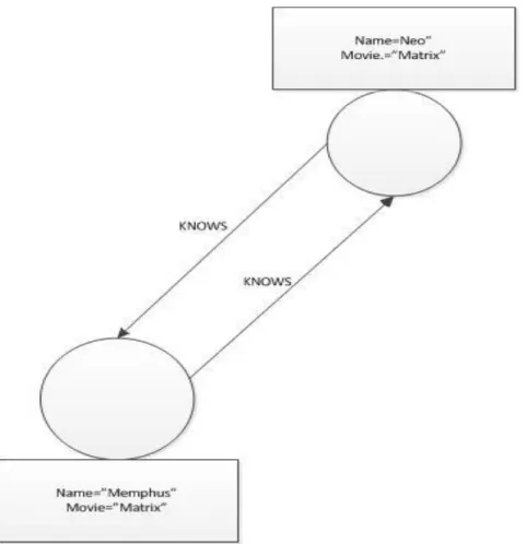
A graph database basically stores data in graph data structure with nodes and edges. The nodes represent objects or entities such as names, book titles, and so on. Edges represent the relationships between nodes. Both edges and nodes can have more than one property.

This figure below shows an example of two nodes connected with a relation

called  “KNOWS”.  

Figure 1.2 An example of a graph database using graph property

1.5

BASE vs. ACID

One of the basic important principles that NoSQL databases based on is BASE and CAP theorem. CAP theorem (Consistency, Availability, and Tolerance of network Partition) was introduced by Professor Eric Brewer in 2000 as a conjecture [22], and later it was proven [23] that a distributed system can only provide any of the two principles

of the CAP theorem for high performance and scalable distributed systems (for example, we can have a distributed system that has high availability and is tolerant of network failure, but we have to sacrifice consistency ).

The B.A.S.E theorem [24] evolved from the needs of the CAP theorem. It is totally different from the ACID properties. BASE is Basically Available, Soft State, and Eventually Consistency.

 Basically Available: This means that data is available through multiple replicas no matter what happens; therefore, data will be available most of the time.

 Soft State: This means  the  store  doesn’t  have  to  be  consistent  at  some  period  of  

time, but eventually the store will be in a consistent state.

 Eventually Consistency: At some periods of time when there are no changes sent to the store, all updates will happen eventually, and all replicas will be in

consistent state. However, the cost of this approach is that  it  doesn’t  offer  a  

guaranteed reliability in real time, but we can expect a high performance distributed system.

ACID provides guaranteed consistency, and database transactions are processed reliably through set of properties:

 Atomic: It’s  either  the  whole transaction has succeeded and will be committed, or the database state stays unchanged and the transaction fails.

 Consistency: If a transaction was completed successfully, the database will go from one consistent state to another consistent state.

 Isolation: This property makes sure that transcations are executed serially for concurrent control of the system. For example, a failure in one transcation might not be visible to another transcation.

 Durability: This means once a transaction was committed successfully, it should be stored permanently to the physical storage, no matters what happen to the database thereafter.

Chapter 2

2

Data Mining

This chapter covers an overview of data mining techniques and algorithms. Section 2.1 covers the concepts behind data mining and its real world applications. Section 2.2 covers the common data mining algorithms and techniques. Finally, section 2.3 covers the pre-processing techniques.

2.1

What’s  Data  Mining?

Data mining is concerned with knowledge discovery and finding patterns in datasets through a process of applying the model to the data [13]. The model, the heart of the data mining process, is the technique and algorithms that are applied to the data to find similarities, patterns, and do data clustering. The common models of data mining are classification, association rules, and clustering. In this research, the focus is on clustering and finding frequent item-sets.

Data mining has a wide range of applications in science and engineering. For example, in weather forecasting , the classification model can be used to predict the weather for the next day based on the previous data. Another example is for movie suggestions in recommender systems. Based on some user’s preferences, other movies that are preferred by the user can be predicted. Clustering model algorithms also have wide range of applications such as scene completion, data summarizations, and data recovery techniques. Finally, frequent item-set is widely used in retail systems to predict customers buying habits, as well as in catalog design.

2.2

Data Mining: The model

As explained earlier, the model is the algorithm that is applied to the data to find similarities, patterns, data summarizations. In this section A-priori algorithm and K-means algorithm are covered in detail.

2.2.1

Apriori Algorithm

A-priori algorithm [26] is one of the common data mining algorithms that is used to find frequent item-sets in transactional databases. A-priori works by finding frequent items from the transactional database domain. Then, the algorithm tries to find the relations or the associations between items.

Suppose there is a transactional database D for a retail store. This store wants to analyze the buying habits of the customers – by finding the relations between the

customers who buy items together in order to help develop a marketing strategy. To do

that,  let’s  define  the  problem  in  a more formal way:

 Let suppose I =  {I1,  I2  …  In}  be an item-set. And D is a transactional database  Let A and B be sets belong to a transaction T (

A, B

⊑

T



A

⊑

B

⊑

o S (Minimum support) is taken as 𝑃(𝑨   ∪ 𝑩).

 S  (A ⟹ 𝐁) =  P(𝐀   ∪ 𝐁)

 𝐶  (𝐴 ⟹ 𝑩) =  𝑃(𝑨  |𝑩) = 𝑺𝒖𝒑_𝑪𝒐𝒖𝒏𝒕(𝑨  ∪𝑩)_{𝑺𝒖𝒑_𝑪𝒐𝒖𝒏𝒕(𝑨)}

A-priori algorithm was developed at IBM by Agrawal [26] for finding frequent item-sets in transactional databases. The pseudo code of the algorithm as it was published is below:

Sequential Apriori Algorithm Ck: candidate itemset of size K.

Lk: frequent itemset of size K

L1: {frequent itemset} // 1-itemset by scanning D.

For (K=1, Lk !=  , K++) do begin

Ck+1 = candidates generated from Lk ;

For each transaction t in D do // scan the database for support count. Increment the count of all candidates in Ck+1 that are in t

Lk+1 = candidates in Ck+1 with minimum support.

End Return ∪_𝒌  𝑳_𝒌 ;

 Join step: Ck is generated by joining Lk-1 with itself.

 Prune step: any (k-1) item-set that is not frequent, its subs so is not frequent. As shown above, the algorithm works as follows:

 At first, the whole database is scanned to determine the item counts in the database D (1-itemset or L1).

 Then, the algorithm will join (L1) with itself to produce the next frequent item-set (k-itemset). Two frequent items are joinable if their (k-1) are matched.

 Finally, the algorithm iterates until Lk is empty.

A priori property

All nonempty subsets of a frequent item-set must also be a frequent.

Suppose we have the set of items while finding the frequent items, I = {I1, I2, I3}; if all the subsets of the set I frequent ({I1, I2}, {I2, I3}, and {I1, I3}), the set I should also be frequent.

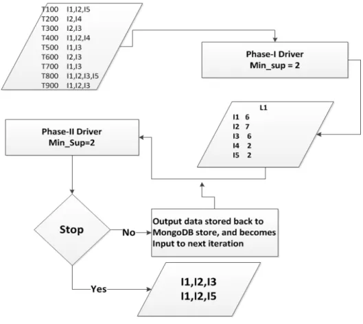
To understand the algorithm, an example is given below:

TID

100

I1,I2,I5

200

I2,I4

300

I2,I3

400

I1,I2,I4

500

I1,I3

600

I2,I3

700

I1,I3

800

I1,I2,I3,I5

900

I1,I2,I3

L1

Sup_count

{I1}

6

{I2}

7

{I3}

6

{I4}

2

{I5}

2

L2

Sup_count

{I1,I2}

4

{I1,I3}

4

{I1,I5}

2

{I2,I3}

4

{I2,I4}

2

{I2,I5}

2

C2

Sup_count

{I1,I2}

4

{I1,I3}

4

{I1,I4}

1

{I1,I5}

2

{I2,I3}

4

{I2,I4}

2

{I2,I5}

2

{I3,I4}

0

{I3,I5}

1

{I4,I5}

0

C3

Sup_count

{I1,I2,I3}

{I1,I2,I5}

{I1,I3,I5}

{I2,I3,I4}

{I2,I3,I5}

{I2,I4,I5}

C3

Sup_count

{I1,I2,I3}

{I1,I2,I5}

L3

Sup_count

{I1,I2,I3}

2

{I1,I2,I5}

2

2.2.2

K-means Algorithm

Clustering is another important data mining model. Clustering is widely used in image processing, scene completion and more. There is more than one algorithm as an implementation for clustering technique; one of the important ones is K-means algorithm.

K-means works by partitioning the data into k clusters; each feature or

observation is closely similar to each other in one cluster, and dissimilar from the features of the other cluster based on some metric distance. A metric distance can be any metrics measure such as Jaccard similarity, cosine similarity or Euclidian distance. Euclidian distance is used mostly with numerical data type. For example, Euclidian distance is used in image processing to cluster the similar photos together as one cluster.

Example:

Suppose one needed to partition the size of the T-shirts into {Small, Medium, and Large}. The data was collected by asking each person to give their best fit size (numeric), height, weight, and so on. Each person or object can be represented as a vector of a d-dimensional space. A collection of the dataset can have N objects.

Obj1        [d11,  d12,  d13  ….d1d] Obj2        [d21,  d22,  d23  ….d2d]

…….

The data can be partitioned based on computing Euclidian distance between each object feature and the cluster center.

𝐷

    = 𝑠𝑞𝑟𝑡(𝑋 − 𝑋 ) +  (𝑌 − 𝑌 ) +  … … + (𝑍 − 𝑍 )

(t) is the number of iteration, and c(i) is the cluster center.

The cluster center is selected randomly from the data domain for the first iteration. And then, each new center for the next iteration is going to be the mean of the cluster of its objects. It can be calculated as below:

Since we are dealing with a d-dimensional vector, the new center is going to be the mean of each dimension divided by number of objects in that cluster.

𝑀𝑒𝑎𝑛  (𝑚) =  …..   The new center is [m1, m2….  md]

The pseudo code of the algorithm as shown below:-

Pseudo code

Sequential K-means Algorithm

Input:

 K: the number of cluster

 D: a dataset containing n objects. Output: A set of k clusters.

Method:

(1) Arbitrarily choose K objects from D as the initial clusters; (2) Repeat

(3) Re-assign each object to the cluster based on the closet mean value of that cluster;

(4) Compute each cluster means (5) Until no changes;

2.3

Data mining: Pre-processing

Real data have different varieties of structure such as photos, sensors data, and texts. Also, data come from different sources, which need to be integrated from multiple sources. Real data are also dirty, noisy, and incomplete, so there are four general

guidelines for pre-processing techniques:

 Data cleaning: Real data are incomplete and require filling missing data, smoothing outliers, and fixing inconsistencies.

 Data transformation: Data needs to be normalized or made into one form.  Data integration: Sometimes  it’s  required  to  integrate  data  from  multiple  

sources.

 Understand different data types: Data has different formats and structures such as numerical data, nominal data, binary data, and so on.

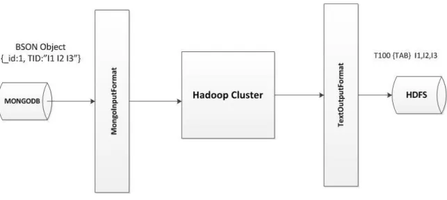
To understand the pre-processing in action, in this research work the data were generated as BSON format to be stored in MongoDB stores, and the algorithm were coded to consume instances from MongoDB. But then to implement the same algorithm on HDFS (Hadoop distributed File System), data need to be converted to plain text so it can be stored and processd on HDFS. The steps below show how the pre-processing was done:

 The data are stored in MongoDB store, and then the data are fetched through

MongodbInputFormat to Hadoop cluster.

 The output is stored as a plain text file in Hadoop file system (HDFS).

Chapter 3

Big Data Concepts, Tools, and Design

Big Data requires sets of tools and technologies to be processed efficiently within an acceptable time manner. In this chapter, the underlying technology of Big Data is covered in more detail. Section 3.1 covers what the concept of Big Data is. Section 3.2 covers Hadoop as the core of Big Data technology stack, and how it works. Section 3.3 covers MongoDB as an example of NoSQL databases, and how that can be integrated. Finally, the relation between Big Data and cloud computing and how these work together is explored.

3.1

What is Big Data?

Users generate a lot of data every day. Data come from digital photos, GPS, sensors, and many more sources. All of this data is unstructured or has different varieties of structures. This huge data requires an efficient cost effective storage system, which is also scalable for data growth. IBM defines [30] Big Data as having four dimensions or characteristics (4 Vs of Big Data):-

 Volume means that data are too big, i.e., terabytes or even petabytes of data.  Variety means that data doesn’t  have a relational format or isn’t  stored as a

relational format. Data can be semi-structured (XML, BSON) or even as raw unstructured data such as photos, logs, texts, and so on.

 Velocity is the speed of data processing (real-time). Some applications or decisions are required to be made quickly, such as E6 sensors in surveillance system might able to detect a bank robbery in real-time.

 Veracity means “conformity  with  truth or fact”,  according to the free online dictionary [31] This fourth dimension assure the truthfulness or accuracy of the ouput results for making decisions.

3.2

Hadoop: Core of Big Data

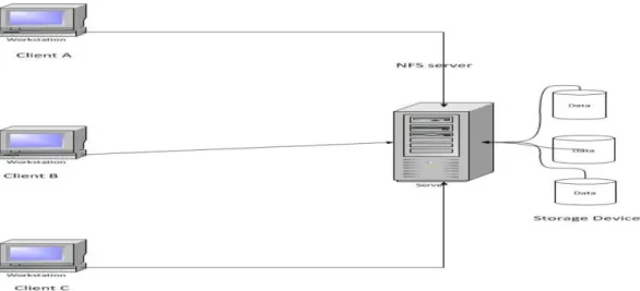
Distributed File Systems (DFS) was not a new concept, but came from the need to share data from a centralized data storage among different clients. DFS basically allows multiple clients to access files remotely on the file server for open (), close (), read (), and other operations. NFS (Network File System) is widely used as a distributed file system over a network. It was developed by Sun Microsystems as open protocol standards. NFS allows clients to access files remotely as they appear as they were stored directly to client storage.

Even though NFS is a powerful distributed file system, it has one main

disadvantage – it stores all its volume data on one single machine. This means that the system has less reliability when the server goes down. Also, there is a storage limitation, the system can only store as much data as the machine can handle.

Today, NFS cannot fill the needs of Big Data. So, Hadoop was designed to store very large data on multiple nodes up to Terabytes or even Petabytes.  So,  what’s  Hadoop and how does it work? Hadoop [32] is an open source implementation of Google File System (GFS) developed by the Apache Project. It was designed by Doug Cutting [32] when he was working with Yahoo. Hadoop uses the Master/Slave model. The master is called Name-Node in the cluster, and it manages the blocks metadata and storage namespace and other requests that come from the clients to the file system. Name-Node also stores information about where those data blocks are stored in the cluster, whereas the slave works mainly as a data-node for storing data blocks as well as a task-tracker for MapReduce computation. There are two major components or layers in the Hadoop system – the HDFS layer and the MapReduce layer. Figure 3.2 below shows an abstract view of Hadoop cluster components.

HDFS layer:

HDFS (Hadoop Distributed File System) is a robust distributed file system that was designed to store very large data – Terabytes, or even Petabytes of data. HDFS splits up large input files into small chunks or blocks. Each block has a fixed size – 64 MB (default). These blocks are distributed and stored on different data nodes in the cluster. MapReduce layer:

The MapReduce layer consists of JobTracker and TaskTracker. JobTracker is responsible for job assignments, task monitoring, job status and so on. TaskTracker, on the other hand, has responsibilities in running Map and Reduce tasks. To understand fully how this process works, the steps done by the framework are the following:

 When the client submits a job, the JobTracker contacts NameNode for data blocks locations.

 The number of Map tasks is determined by how many blocks this specific input file has.

 The JobTracker accordingly assigns Map tasks to the TaskTrackers to run on each data block to produce what is called intermediate key-value pairs. Map tasks store the output to the local file system of that specific node.

 When all Map tasks finish, the sorting, grouping and shuffle based on keys are done by the framework; similar keys merged together to become a one key and a list of associative values. Then each Reduce task consumes part of the shuffled data and output back to HDFS.

 When all Reduce tasks finish, all intermediate data stored in temporary files are deleted upon the successful completion of the job.

To understand this process more, a word count example using MapReduce is explained in the figure below:

Figure 3.3 A diagram of Word-Count example using Hadoop-MapReduce [34].

Hadoop MapReduce consumes data as raw text or even as a sequence binary format for a fast data transfer. Hadoop has its own data types that differ from Java, which are IntWritable, LongWritable, Text, ArrayWritable, and others. All data types in Hadoop

implement Writable, the interface for serialization. Hadoop uses its own serialization implementation. The Writable Interface has two methods, write and read as shown below:

However, some complex MapReduce implementation requires having a custom data type that is not available in Hadoop. Fortunately, by using the Writable interface,

custom data type is possible. For instance, in Chapter 4, in K-means algorithm

implementation, a vector of each cluster emitted is associated with a cluster ID. Vectors having the same cluster ID will be grouped together as one cluster through the

MapReduce process. A vector is a one-dimensional array of size N. The following code snippet is shown below for InVectorWritable data type:

A custom data type needs only to implement writable interface, and how an object can be serialized and de-serialized. An array object [27, 35] can be serialized by writing to output stream the array size and its contents. Conversely, it can be de-serialized by reading from the input binary stream the array size and its contents.

3.3

MongoDB: a NoSQL example

MongoDB [1] is schema-free, document-oriented, non-relational databases (NoSQL). It was written in C++ by 10gen Corporation as an open source project. MongoDB architecture has three core components:

 Mongod process handles data request and manages the underlying data format and data store.

 Mongos is the routing controller service for shard cluster. It handles incoming request from application layer in shards cluster and generates a response.  Mongo is a JavaScript shell that helps the administrator to perform a wide

range of query operation for testing, among others.

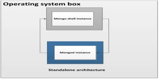
Figure 3.4 Standalone architecture of MongoDB.

The figure above shows simple standalone architecture and how MongoDB works. An administrator starts a mongod instance for handling data request and listens on

“127.0.0.1”  IP  address  if  it  is on a local machine (default port is 28017). Then mongo

instance is started and interactively sends back and forth requests to mongod instance.

MongoDB uses BSON (Binary Simple Object Notion), a binary encoded format of JSON. BSON supports the same data types that JSON supports. A BSON document can store strings, numbers, arrays, data objects, and even another BSON document.

However, MongoDB stores each BSON document with a unique id called object-id. An

example of a BSON document is shown below:

Although it was mentioned earlier that MongoDB has flexible schema design, in practical applications, developers need to take a flexible schema and data modeling into consideration. MongoDB database can have many collections (representing tables in relational databases), and each collection can have many documents. Collections do not require or impose any constraints on document structure. Nevertheless, some

recommendations follow for data modeling in MongoDB:

Mongo-DB Data modeling

In practical applications, schema design is a very important factor of any database management system. In MongoDB, as it has dynamic schema design, documents in real applications share similar structure for good performance. There are patterns techniques required as follows:

 Embedding (similar to de-normalization). This means that instead of having many one-to-one relationships among documents, by embedding those other documents into one gets a better read performance. In this case, a read operation can be done in a single query, for instance, student enrollment at a university. The university keeps records of the  student’s  names, their education, and their

addresses. Each one is a separate document.

However, by using the embedding technique, a read operation about a student’s  records  

 Referencing (normalization), is used in the case of one-to-many relationship among documents. For example, a hospital stores information about its doctors. Each doctor has many patients. The first scenario is to store an array object in the doctor’s  

The second scenario is to reference on each patient document the doctor’s id.

 MongoDB supports atomicity on a single document level for write operations. For

that  reason,  it’s  sometimes better to use an embedding data model to insure this property when  it’s  required  by  the  application.  For  instance,  in the example about a student’s  record,  atomic  update  can  be  done  quickly. The document can be found based on the student id and through set expression – the subdocument

“education”  also  can  be  changed  as well. As in the example below, the status value was changed, and another new field was added simultaneously.

Above, it was simply explained how the MongoDB works, but what about scalability? How do MongoDB clusters work? The MongoDB is horizontally scalable (scaling-out model), and there are two kinds of distributed architecture for the MongoDB:

1. Replica-Set Cluster

MongoDB supports automatic failover in replica-set cluster. Replica-set architecture allows MongoDB to replicate its data across multiple nodes to insure high data

availability (Basically Available). Each node runs its own mongod instance. The

Replica-set model is similar to the Master/Slave  approach;;  however,  Master/Slave  doesn’t  support  

automatic failover. When the Master goes down, an immediate intervention is required. Replica-set model has primary node (Master) and can handle up to 12 nodes in the cluster. All read and write operation are handled by the primary one and propagate any changes to all other secondary nodes (eventual consistency). In case of failover or if the primary goes unreachable, the secondary members trigger an election. When a secondary gets a majority votes, it becomes the primary. For example, suppose a replica-set (A) has

three nodes, one primary and the other two secondary. Figure 3.5 shows a replica-set cluster with three members, one primary and the other two secondary.

Figure 3.5 A MongoDB replica-set architecture with three members

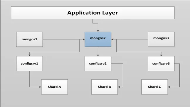
2. Shard Cluster

MongoDB is a horizontally scalable database. MongoDB allows sharding on a collection level. A collection is partitioned to smaller chunks based on shard keys. A shard is a collection of documents within the shard key range. Furthermore, each shard can be partitioned to smaller chunks if the size of the shard exceeds 64 MB, also within the key range. The shard key is a similar field across all the documents within a

collection. A shard key could be indexes or document ids. To deploy a shard cluster, these steps are followed:

1. To enable a shard cluster on a database, it requires three mongod instances that work

as a layer above the shard nodes. Each configsvr runs on its own machine. Those three mongod store the chunks of metadata and that’s  where they are located.

2. At least three mongos instances run on a different machine each for reliability. Mongos instance cache and store the metadata of the configsvr and route all read and write operations to its shard container.

3. Shard containers can have either one mongod instance or a replica-set of mongod

instances for high availability.

Figure 3.6 below shows the architecture of a shard cluster. It has three mongos

instances, three configsrv, and multiple shard containers.

3.4

Big Data and Cloud Computing

Cloud computing is new information technology model that has helped to revolutionize IT development, cost and infrastructure. Cloud computing has three main types of architecture. First, the SaaS (Software as a Service) model means that an organization can sell its software online, accessible through the Web. This model helps to reduce software cost and provides ease of managing software licensing. An example is 10gen Company [38], which provides storage as a service for mongo-db enterprise edition for backup and recovery. The software agents are installed on the mongo-db server and take data snapshot every 6 hours.

The second model is PaaS (Platform as a Service), which means the cloud providers have their own computation resources, but the clients can access and benefit them from the platform through an API. An example is Facebook, and clients can even develop online games, apps, and so on.

Finally, IaaS (Infrastructure as a Service) provides access to computation resources. Cloud users can spawn instances of Linux OS, install on it anything, and connect it to the world. A simple example is this research implementation; the Hadoop cluster is running on 5 Linux VMs on the BU server.

From all  that’s  been  said,  cloud computing is considered a utility as a service, or pay-as-you go model, which is  what’s  required  for  Big Data retrieval and analytics.

Big Data for a large organization such as Wal-Mart or Netflix requires thousands of nodes and high performance computing. By using cloud infrastructure, Big Data technology is easily implemented. Thus, cloud computing is an important player and a necessity in Big Data future and technology.

Chapter 4

Implementations and Results

This chapter shows how the Hadoop/MapReduce paradigm can be used for application developments. Two algorithms of data mining were implemented using Java language. The implementation was done on 5 nodes of virtualized platform on BU MET IT server (Boston University). Each node is a BU-Linux OS (CentOS) 64 bits; 4 GB of RAM; each node has 4 processors, each of which is 2 GHZ and 4 cores. Section 4.1 covers the implementation and results of the two algorithms with MongoDB data store. Section 4.2 covers the implementation and the results of the two algorithms on HDFS (Hadoop File System). The Hadoop version that was used is hadoop-0.20.2. The Java code of the algorithms implementation can be found in Appendix A.

4.1

MongoDB Data Store

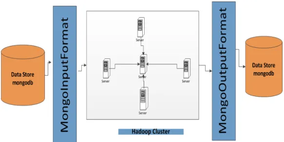
As explained in Chapter 3, MongoDB is an open source, document-oriented, schema free database that stores data as a BSON documents. Each database may have multiple collections. Each collection may have many documents. MongoDB comes with open source connector that is used to fetch data from MongoDB as a BSON document. The data is read from MongoDB by using MongoInputFormat. The MapReduce

computation is done in Hadoop cluster, and then the output is stored back into MongoDB cluster through MongoOutputFormat. Figure 4.1 below shows the implementation of MongoDB and Hadoop Cluster.

Figure 4.1 An Implementation of MongoDB cluster with Hadoop Cluster.

4.1.1

Apriori-MongoDB Algorithm

As mentioned earlier in Chapter 2, Apriori Algorithm is a data mining technique that is used to find frequent item-sets in transactional database. The algorithm is

computationally expensive. To Implement Apriori with MapReduce, we need to understand how it works:

1. The first step is to find L1, which basically counts all the item in the database.

This step is very straightforward in MapReduce.

a. In Map Task, each document will input to the map (Key, Value) function. The key is items, and the value is one.

b. The Reduce Task, after shuffling and sorting the data, is based on keys. The Reduce (Key, Value []) function. The key is the item, and the value is

a list of counts of that item. The Reduce task will iterate over the value and output the final sum.

2. When the level is 2, join is required to find the next level. This can be done in Map task. Reduce task will find the final sum of the items, and filter them based on minimum support.

3. Stopping criteria if Lk is empty. This can be done easily by checking the stop flag

using an if-statement.

Pseudo Code

Phase –I: find L1

FirstMapper

Input: D the transactional database as a BSON documents. Key: is the document id; Value: items

Output: Key: items; Value: count of one. 1. Read items from BSON object.

2. Construct Key as the item. 3. Value is count of one. 4. Context.write (item, one).

FirstReducer

Input: Key: items; Value: list of counts. Output: L1 1. Counter = 0; 2. Iterator. While (value.hasNext){ Counter + = value.next; }

3. Construct Key as the item; 4. Prune based on min_sup. 5. Value = counter;

Phase-II

AprioriMapper

Input: Lk-1 and scan database; Value: BSON documents. Key: documents id.

Output: Ck; Key: items; Value: count;

1. Read Lk-1 from MongoDB.

2. Ck = Join Lk-1 X Lk-1 ;

3. Prune step before scan D. 4. Construct Key as item 5. Value is count of one. 6. Context.write();

AprioriReducer

Input: Key as items; Value: list of counts. Output: ∪𝒌  𝑳𝒌 1. Counter = 0; 2. Iterator. While (value.hasNext){ Counter + = value.next; }

3. Construct Key as the item; 4. Prune based on min_sup. 5. Value = counter;

6. Context.write (Key, counter); // stored in MongoDB store as BSON. 7. If 𝑳_𝒌 is empty. Stop.

Results

For the simulation purposes and to show the algorithm performance, the data was generated using a Java program. The code is available in Appendix D. The table below shows different experiments performed to gauge the A-priori Algorithm performance with MongoDB data store. Also, each experiment was done on a different dataset.

ID Universal Items in a store Total items in database Num items/ trans Num Map/ Reduce Tasks Split size Frequent item-set found Total time/minutes Dataset size

E1M20I100 100 item 1 million 20 4/5 64

MB L3 33.90 Min 117 MB

E1M30I10K 10,000 1 million 30 5/5 64

MB L2 494 Min 168 MB

E2M10I100 100 item 2 million 10 7/5 64

MB L3 30.55 Min 181 MB

E3M20I1K 1000 3 million 20 11/5 64

MB L2 247.81 Min 408 MB

4.1.2

Kmeans-MongoBD Algorithm

means Algorithm is another one of the common data mining techniques. K-means algorithm partition the data into clusters based on some metric distance. Each object in one cluster is similar to each other, and dissimilar from other clusters. In Chapter 2, K-means was covered in more detail.

To implement K-means algorithm in MapReduce is according to the following:  After picking a number of clusters as the initial step, the algorithm assigns each object to the closest cluster mean based on Euclidian distance. This task can be done in Map task :

o Assign each object to closest cluster center.

o Compute distance – using Euclidian distance.

 After each object was assigned to a cluster, the next step is to compute the new cluster mean for the next iterations until there are no further changes in the cluster mean.

o This task can be done in Reduce task where each cluster will be input to a Reducer task since its all objects have the same cluster ID.

Pseudo Code Map Function

Input: Key: document id; Value: BSON document. Cluster center globally to all nodes. 1. Read center from distributed cache center[];

2. minDist = 9999;

3. For int i=0; I <center.length; i++; j=0; {

Int d = computDistance (value [j], centroid[i]); If (d < minDist) { minDist = d; } cluster_id = i; J++; }

4. Construct key as index;

5. Value as a d-dimensional vector. 6. Context.write (cluster_id, Vector); Reduce Function

Input: key : ClusterId, Value :list  of  vector’s  objects.

Output : data clusters; and new cluster mean.

1. numOfPoints = 0; // to keep track number of point to compute the mean 2. read value [];

3. while (value.hasNext){

output(clusterId, cluster objects ) Sum + = sum + value. Next; }

Center = sum / numOfPoints //compute the cluster mean as a new center. 4. Key as a key;

5. Value list of vectors;

The pseudo code above is very straightforward. During the Map task, based on the metric distance, the observation is assigned to a cluster. In the Reduce task, the new mean is calculated until there are no changes, and for some iterations, the algorithm stops. The flow chart below explains the process more clearly:

Results

Data were generated using a Java program for simulation and algorithm performance. The Java code can be found in Appendix D. In the table below, each experiment was done on a different dataset.

ID Total data records Num Map/Reduce Split size Number of iteration Number of cluster Total time/minutes Data set size

Ekm3M3C 2 million 12/1 8 MB 3 3 9.2 Min 326 MB

Ekm9M3C 9 million 36/1 8 MB 3 3 36.46 Min 987 MB

Ekm12M3C 12 million 48/1 8 Mb 3 3 44.46 Min 1270 MB

Table 4.2 Performance of K-means MongoDB on Hadoop cluster

4.2

Hadoop Data Store

HDFS (Hadoop Distributed File System) is a distributed file system that is used to store very large datasets. HDFS stores data as blocks or chunks in a data-node. The file system blocks are managed by the primary server (NameNode).

However, to implement K-means and A-priori  Algorithm,  it’s  really  the  same  as the previous section. However, instead of reading the data from MongoDB, the data is read from HDFS, which is more flexible than MongoDB. It supports different data types such as text files or binary sequence files.

4.2.1

K-means Hadoop Algorithm

In Chapter 2, in the pre-processing section, it was shown how we can convert a BSON object to a TEXT file to process the data in the HDFS data store. The

implementation for Hadoop is similar for MongoDB; however, the only difference is that instead of reading the data from MongoDB, here the data is stored and read directly from HDFS. In the table below, each experiment was done on a different dataset.

ID Total data records Num Map/Reduce Split size Number of iteration Number of cluster Total time/minutes

Ekmh3M3C 2 million 1/1 8 MB 3 3 8.31 Min

Ekmh9M3C 9 million 1/1 8 MB 3 3 28.30 Min

Ekmh12M3C 12 million 1/1 8 Mb 3 3 13.30 Min

4.2.2

Apriori- Hadoop

The implementation of A-priori  algorithm  on  HDFS  doesn’t  differ  from  the  

implementation of A-priori MongoDB. The only difference is instead of reading data from MongoDB by using MongoDB adapter, the data is read directly from HDFS. In the table below, each experiment was done on different dataset.

ID Universal Items in a store Total items in database Num items/trans Num Map/Reduce Tasks Split size Frequent item-set found Total time/minutes

E1M20I100 100 item 1 million 20 5/1 8 MB L3 64.2 Min

E2M10I100 100 2 million 10 6/1 8 MB L2 91.11 Min

E2M20I1K 1000 2 million 20 6/1 8 MB L3 68 Min

Chapter 5

Conclusion and Future Work

5.1 Conclusion

Big Data is new field of study in computer science that applies knowledge from different scientific, technical, and practical applications to seek new answers. Smart phones, digital cameras, smart cars, GPS -- of these devices generate huge amounts of data that have a lot of potential for financial return. For instance, GPS data can be used by insurance companies to track their customers where it helps to predict how likely this driver is to get into an accident and so on.

However, Big Data is defined as having four dimensions or 4Vs. Big Data has volume, which means the data are massively large – TBs, PBs and more. Big Data has velocity, meaning that data need to be processed almost in real time. Big Data also has variety, both semi-structured and unstructured. Finally, the fourth dimension of Big Data is veracity, meaning the truthfulness and the accuracy of an inference model for making decisions.

This thesis research encapsulates common Big Data tools and concepts. In Chapter 3, Hadoop, the core of Big Data, was covered in detail. The Hadoop file system can store up to hundreds of Terabytes of data. More importantly, Hadoop implements the MapReduce computation paradigm, a simple yet powerful computing model. It helps

hide the complexity of parallel programming from developers, so they only need to write their Map and reduce function. An implementation of the Hadoop cluster was done through this work – 5 of its nodes  were  deployed  on  MET  IT  VMware’s  server.  

Furthermore, an integration of Hadoop MongoDB was also done as a Big Data technology. Hadoop MongoDB has a high potential, and it is a fully open source. Also, MongoDB can be used to build a real time application on top of it. While the heavy computation can be done offline in a Hadoop cluster, the results can be stored back to MongoDB for presentation.

Finally, an implementation of A-priori Algorithm and K-means Algorithm were done on both data stores – MongoDB and HDFS.

5.2 Future Work

A lot potential for future work is contained in this research, summarized below:  Practical implementation of Hadoop MongoDB technology stack such as

implementing a recommender system on top of MongoDB, with Hadoop used for offline computational power.

 Design of software packages for data pre-processing using Hadoop MapReduce.  Exploration of data visualization for Big Data.

Appendix A Java Code

A.1 MongoDB Data Store

/**

* AprioriDriver : manage which and how each job will run. * it has these method :

* main() to invoke and start the program.

* AprioriGenerator () : this method will be called many times * until the loop stop.

* */ package bu.thesis.bigdata; import java.io.IOException; import java.net.URISyntaxException; import org.apache.hadoop.conf.Configuration; import org.apache.hadoop.conf.Configured; import org.apache.hadoop.fs.FSDataInputStream; import org.apache.hadoop.fs.FileSystem; import org.apache.hadoop.fs.Path; import org.apache.hadoop.io.IntWritable; import org.apache.hadoop.io.Text; import org.apache.hadoop.mapreduce.Job; import org.apache.hadoop.util.Tool; import org.apache.hadoop.util.ToolRunner; import com.mongodb.hadoop.MongoInputFormat; import com.mongodb.hadoop.MongoOutputFormat; import com.mongodb.hadoop.util.MongoConfigUtil; /** * @author Idrees * */

public class AprioriDriver extends Configured implements Tool {

@Override

public int run(String[] args) throws Exception {

//parse the commandline

if(args.length != 1){

System.err.println("Method Usage:

bin/Hadoop Jar Apriori.jar <min_sup>"); ToolRunner.printGenericCommandUsage(System.err);

return -1; }

//conf object

Configuration conf = new Configuration();

//set input uri for the mongodb to fetch data.

//(apriori) db name; in (collection name: input as a BSON format)

MongoConfigUtil.setInputURI(conf,"mongodb://128.197.103.44/apriori. in3M1KI");

//set output uri for mongodb cluster.

//this address for primary server of the replica set cluster.

MongoConfigUtil.setOutputURI(conf,"mongodb://128.197.103.44/ apriori.L1");

//set inputSplitSize to 64mb (hadoop default)...

//mongodb default is 8mb .. to reduce number of Mapper tasks.

MongoConfigUtil.setSplitSize(conf, 64);

//Apriori Phase-I

Job job = new Job(conf);

job.setJobName("HadoopApriori - in3M-1KI");

//Jarclass.

job.setJarByClass(AprioriDriver.class);

//set the value output and the key output class

job.setMapOutputKeyClass(Text.class);

job.setMapOutputValueClass(IntWritable.class);

//set map and reduce class.

job.setMapperClass(FirstAprioriMapper.class); job.setReducerClass(FirstAprioriReducer.class);

// input/output format class

job.setInputFormatClass(MongoInputFormat.class); //job.setInputFormatClass(cls) job.setOutputFormatClass(MongoOutputFormat.class); job.setNumReduceTasks(5); //run job job.waitForCompletion(true);

//iterate over Lk until no items left. //stoping criteria checks stop.txt {stop}

FileSystem fs = FileSystem.get(conf2);

int loop = 0;

int k = 2;

boolean stop = false;

boolean check = true;

while(!stop){

loop = AprioirGenerator(k,conf2);

if(check){

String st = "STOP"; String by;

if(fs.exists(new Path("stop.txt"))){

FSDataInputStream in = fs.open(new Path("stop.txt")); by = in.readUTF(); if(st.equals(by)){ stop = true; check = false; } in.close(); } } k++; } return loop; }

private int AprioirGenerator(int k, Configuration conf)

throws IOException,ClassNotFoundException, InterruptedException, URISyntaxException {

conf.setInt("L", k); System.out.println(conf);

//set input uri for the mongodb to fetch data.

//(apriori) db name; in (collection name: input as a BSON format).

MongoConfigUtil.setInputURI(conf, "mongodb://128.197.103.44/apriori.in3M1KI");

//set output uri for mongodb cluster.

//this address for primary server of the replica set cluster.

MongoConfigUtil.setOutputURI(conf, "mongodb://128.197.103.44/apriori.L"+k); MongoConfigUtil.setSplitSize(conf, 64);

Job job = new Job(conf);

//Jarclass.

job.setJarByClass(AprioriDriver.class);

//set the value output and the key output class

job.setMapOutputKeyClass(Text.class);

job.setMapOutputValueClass(IntWritable.class);

//set map and reduce class.

job.setMapperClass(ApriorMapper.class); job.setReducerClass(AprioriReducer.class);

// input/output format class

job.setInputFormatClass(MongoInputFormat.class);

//job.setInputFormatClass(cls)

job.setOutputFormatClass(MongoOutputFormat.class);

//double num of reducers/node. to boost the performance.

job.setNumReduceTasks(5); //run job job.waitForCompletion(true); return 1; } /** * @param args * @throws Exception */

public static void main(String[] args) throws Exception {

int exitcode = ToolRunner.run(new AprioriDriver(), args); System.exit(exitcode);

} }

/**

* input. D is a transcational DB of a BSON file. * Key: BSON document; Value : I1,I2,I3 ....

* output : (item , 1). Key : as an item; value : as a count of one. */ package bu.thesis.bigdata; import java.io.IOException; import org.apache.hadoop.io.IntWritable; import org.apache.hadoop.io.Text; import org.apache.hadoop.mapreduce.Mapper; import org.bson.BSONObject; /** * @author Idrees * */

public class FirstAprioriMapper extends Mapper<Object,BSONObject,Text,IntWritable> {

//from each Key/Value pairs in each record from the inputSpilts //count each item as (1), then the reducer will sort by Key, and sum the total.

private final static IntWritable counts = new IntWritable(1);

private Text item = new Text();

@Override

protected void map(Object key, BSONObject value, Context context) throws

IOException,InterruptedException {

//input Key is the doc _id (objectId). //Value is the I1,I2,I3...

String line = value.get("TID").toString(); String [] split = line.split(",");

for(int i = 0; split.length > i; i++){

item.set(split[i]);

//emit item, 1

context.write(item, counts); }

} }

/**

* Input: Key:itemset; Value : list of counts of that itemset. * output: L1, 1-itemset. */ package bu.thesis.bigdata; import java.io.IOException; import org.apache.hadoop.io.IntWritable; import org.apache.hadoop.io.Text; import org.apache.hadoop.mapreduce.Reducer; /** * @author Idrees * */

public class FirstAprioriReducer extends Reducer<Text, IntWritable, Text, IntWritable> {

private static final int min_sup; //set by user.

@Override

protected void reduce(Text Key,Iterable<IntWritable> value, Context context)

throws IOException, InterruptedException{

int sum = 0;

for(IntWritable val : value) sum+=val.get();

//prune based on the min_sup.

//and emit only the ones that only satisfy the min_sup.

if( sum >= min_sup)

context.write(Key, new IntWritable(sum)); }

/**

* input: D as BSON documents * Key: document id.

* Value: line-content; I1,I2,I3,.... * output: (itemset, one)

*/ package bu.thesis.bigdata; import java.io.IOException; import java.net.UnknownHostException; import java.util.ArrayList; import java.util.Iterator; import org.apache.commons.logging.*; import org.apache.hadoop.conf.Configuration; import org.apache.hadoop.io.IntWritable; import org.apache.hadoop.io.Text; import org.apache.hadoop.mapreduce.Mapper; import org.bson.BSONObject; import com.mongodb.DB; import com.mongodb.DBCollection; import com.mongodb.DBCursor; import com.mongodb.MongoClient; /** * @author Idrees * */

public class ApriorMapper extends

Mapper<Object,BSONObject,Text,IntWritable> {

private static final Log log = LogFactory.getLog( AprioriReducer.class );

int level ;

private static final IntWritable one = new IntWritable(1);

private Text item = new Text();

ArrayList<String> sublist = new ArrayList<String>();

//Join

private static ArrayList<String> Lk_1 = new ArrayList<String>();

/**

* @param context

* @return Configuration object

* called once at the beginning of the Mapper task. * */

@Override

protected void setup(Context context) throws

IOException, InterruptedException {

log.info("job setup started.");

Configuration conf = context.getConfiguration();

level = Integer.parseInt(conf.get("L"));

//get the Lk-1 from db.

MongoClient(level-1); //get Itemset based on the current level.

//join 1-itemset.

if(level == 2){ join();

log.info("Join been called, level 2"); }

//join k-itemset, where k > 2

else{

join2(level); }

super.setup(context); }

private void MongoClient(int level) throws UnknownHostException {

//read data from master Ip address.

MongoClient mongoClient = new MongoClient( "128.197.103.44" , 27017 );

DB db = mongoClient.getDB("apriori"); //give the database name.

DBCollection dbCol = db.getCollection("L"+level); //get the collection name.

DBCursor cursor = dbCol.find(); //get a cursor over the collections docs.

BSONObject bson = null;

int i = 0; while(cursor.hasNext()){ bson = cursor.next(); Lk_1.add(i, bson.get("_id").toString()); i++; } mongoClient.close(); }