3D Ground Truth Generation Using Pre-Trained Deep Neural Networks

(1)

3D Ground Truth Generation Using

Pre-Trained Deep Neural Networks

by

Jungwook Lee

A thesis

presented to the University of Waterloo in fulfillment of the

thesis requirement for the degree of Master of Applied Science

in

Mechanical and Mechatronics Engineering

Waterloo, Ontario, Canada, 2019

c

(2)

Author’s Declaration

I hereby declare that I am the sole author of this thesis. This is a true copy of the thesis, including any required final revisions, as accepted by my examiners.

(3)

Abstract

Training three-dimensional object detectors on publicly available data has been limited to small datasets due to the significant effort required to generate annotations. The difficulty of labeling in 3D using 2.5D sensors, such as LIDAR, is attributed to the high spatial reasoning skills required to deal with occlusion and partial viewpoints. Additionally, the current methods to label 3D objects are cognitively demanding because they require fre-quent task switching. Reducing task complexity and the amount of task switching done by annotators is key to reducing the effort and time required to generate 3D bounding box annotations. The following work seeks to reduce the burden on the annotators by leverage existing 3D object detectors.

This work introduces a novel ground truth generation method that combines human supervision with pre-trained neural networks to generate per-instance 3D point cloud seg-mentation, 3D bounding boxes, and class annotations. The annotators provide object anchor clicks which behave as seeds to generate instance segmentation results in 3D. The points that belong to each instance are then used to regress object centroids, bounding box dimensions, and object orientation. The deep neural network model that is used to generate the segmentation masks and bounding box parameters is based on the PointNet architecture.

The following method relies on the existing KITTI dataset to analyze the quality of the generated ground truth. The neural network model is trained on the KITTI training split and the 3D bounding box outputs are generated with annotation clicks collected from the validation split. The validation split of KITTI detection dataset contains 3,712 frames of pointcloud and image scenes, and it took 16.35 hours to label with the method used in this study. Based on these results, the proposed approach is 19 times faster than the latest published 3D object annotation scheme. Additionally, the annotators spent less time per object as the number of objects in the scenes increases, making our apporach a very efficient for multi-object labeling. The quality of the generated 3D bounding boxes, using the proposed method is compared against the KITTI ground truth. The model performs on par with the current state-of-the-art 3D detectors, and the labeling procedure does not negatively impact the output quality of the bounding boxes. The proposed scheme is also applied to previously unseen data from the Autonomoose self-driving vehicle to demonstrate the generalization capabilities of the network.

(4)

Acknowledgements

I would like to thank Prof. Steven Waslander for the countless opportunities that he gave me in the field of autonomous robotics. His optimistic and enthusiastic attitude towards research has been a positive influence during my time working in the Waterloo Autonomous Vehicle Laboratory. I would also like to thank all my colleagues in WAVELab for the wonderful times we had working with together. I would especially like to thank Sean Walsh for the cooperative work that we managed to accomplish despite the hard times. I would also like to express my thanks to Ali Harakeh for introducing and mentoring me in machine learning and computer vision. Finally, I would like to dedicate this work to my parents and my little sister for always believing in me.

(5)

List of Figures

2.1 Pooling Layer Visualization . . . 8

2.2 Dropout Visualization . . . 10

2.3 PointNet Architecture Diagram . . . 14

2.4 Frustrum Pointcloud Generation . . . 16

2.5 Frustrum Pointnet Architecture . . . 17

2.6 Frustrum Pointnet Coordinate Transforms . . . 18

2.7 Click Supervision . . . 19

2.8 Sun RGB-D Labelling . . . 20

3.1 Overview of 3D Data Labelling Procedure . . . 23

3.2 Click Collection GUI . . . 25

3.3 Training Feedback GUI . . . 26

3.4 Label3D Ground Truth Generation Architecture . . . 33

4.1 Annotation Time vs. Number of Objects Per Scene . . . 36

4.2 Instance Segmentation Results . . . 39

4.3 Error Case for Segmentation . . . 41

4.4 Histogram of Bounding Box IOUs . . . 44

4.5 Histograms of Car Bounding Boxes Z-axis Distances based on IOU. . . 44

4.6 Histograms of Bounding Box Orientation Errors for KITTI Validation . . . 45

(9)

4.8 Histograms of bounding box size errors for KITTI Validation . . . 47

4.9 Autonomoose Labelling Results . . . 48

(10)

List of Tables

3.1 Instance Segmentation PointNet Layers . . . 29

3.2 Center Regression T-Net Layers . . . 30

3.3 3D Bounding Box Regression PointNet Layers . . . 31

4.1 Comparison of Test Datasets for Annotation . . . 34

4.2 Precision and Recall Performance On Car Class for KITTI Validation Set . 37 4.3 Statistics on Miss Rates . . . 38

4.4 Qualitative Performance Evaluations . . . 40

(11)

Chapter 1 Introduction

1.1 Motivation

In recent years, deep learning has emerged as a dominant approach for improving per-formance on perception tasks related to autonomous driving. This rise has been made possible by unprecedented access to massive, highly parallelized computing infrastructure, and to ever expanding datasets, which enable deep networks to distill complex patterns from noisy sources. For example, the introduction of the ImageNet Large Scale Vision Recognition Challenge [36] led to breakthrough deep learning models such as GoogLeNet [40] and ResNet[11] that have been shown to reach close to human performance in image classification. Similarly, the KITTI Vision benchmark suite shows results of models with ever improving performance for autonomous driving related tasks, and has led to robust progress in diverse areas from pose estimation to object detection, depth estimation and others.

Large datasets are a particularly important factor to achieving good generalization performance for deep neural networks. As dataset size increases, the transformations and variations inherent in the base data are better distilled in the learning process, leading to stronger performance on a given task without any change to the network configuration. For example, in object recognition tasks in 2D images, representations of a single object can have various forms. An image of a car can have numerous variations in appearance, geometric variation, and the sensor used to generate the information are susceptible to noise. A large, representative dataset will contain more of the possible variations, and require the learned representation to handle these variations correctly, thereby ensuring that new observations are more likely to be consistent with the learned representation.

(12)

Furthermore, large datasets are necessary to highlight progress in the development of algorithms used in autonomous vehicles. The datasets can be used to provide a stan-dardized benchmark for comparative analysis amongst the large variety of new algorithms being proposed. Quantitative measures such as the average precision (AP) are commonly used as the metric to determine and compare object detection performance. These metrics provide useful insight into quantifiable algorithmic performance gains, and lead to higher confidence prior to on-road deployment.

Additionally, having multiple datasets from different domains is critical to ensuring that the algorithms are not over-designed to accommodate to specific inherent biases in any particular dataset. Large and varied datasets are still the primary resource to provide generalization and overfitting analysis for deep networks and there is an ever-increasing demand for larger datasets, especially in the field of autonomous driving.

Despite the strong demand, the availability of large autonomous driving datasets re-mains limited. Currently, the most widely used dataset in the domain of autonomous driving is the KITTI dataset [7]. It is frequently used in the literature to prototype and provide comparative analysis for a range of perception challenges. The KITTI dataset contains about 30,000 instances of labelled vehicles with high quality bounding box anno-tations. Due to its small number of label instances and the lack of variety of the scenarios, it cannot provide the adequate generalization performance required to ensure safety for public tests in other environments. Amongst the more recent publications of autonomous car datasets, ApolloScapes[13] has increased the magnitude of instances of vehicle in their dataset to 2 million. However, ApolloScapes lacks high quality 3D bounding box anno-tations and is not widely available. Evidently, the collection of the data itself is not the primary reason why autonomous driving datasets are hard to publish. The bottleneck is caused by to the difficulty and the cost required to obtain high-quality annotations.

1.2 Challenges

Specifically, inferring 3D bounding boxes for all relevant objects in a scene is difficult to annotate using unprocessed 2.5D range data. The data available to annotators from range scanners is sparse [42], and captures surface information only from the sensor’s viewpoint. Depending on the position of the sensor, the object to label will not be fully observable which forces the annotators to rely on mental imagery and spatial reasoning. Additionally, occlusion, missing parts, extent estimation and consistency across multiple frames are common problems in 3D labelling procedures. Thus, human annotators spend much of

(13)

their mental effort in compensating for such ambiguities and incomplete data. leading to long labelling times per object, with high probability of inaccuracies.

To further complicate the task, 3D bounding boxes labelling methods, such as [38], involve frequent task switching. It takes more time to complete tasks if a human must switch between them than if each task is completed for all instances before switching to the next [8]. Furthermore, humans tend to exhibit higher error rates when task switching, when compared to performing one task at a time [28]. Also, task switching is cognitively demanding, resulting in mental fatigue after multiple iterations, which in turn decreases the annotators’ performance [41]. Therefore, elimination of task switching is key to maintaining quality of annotation and an effective way to reduce the burden on the annotators.

Ultimately, the current methods to obtain high quality annotations for 3D bounding boxes rely too much on human effort. Reducing human effort can greatly reduce the time and cost of labelling, since it is the costliest component of the overall procedure. The more difficult the task becomes, the more the cost is increased due to the added time to complete the task, so task complexity must be reduced as much as possible. Research has shown that proper usage of pre-trained networks and object detectors can greatly reduce human effort in labelling frameworks in 2D images [30, 32, 31].

Autonomous driving needs 3D labels, however, and there is currently a lack of research in literature using detectors to assist annotators tailored towards 3D data. The reason is due to the fact that 3D object detectors are a fairly recent development in computer vision research. As of now, the top performing 3D detection models trained on KITTI achieves up to 73 average precision (AP) on medium difficulty for cars. Unfortunately, this implies that the dependence on human in the labelling framework cannot be completely removed since the quality of annotation is still unmatched by any other methods. Therefore, the main challenge addressed in this thesis lies in identifying ways to simplify the human annotator task as much as possible using 3D object detection networks, while still employing human annotators to boost overall labelling accuracy to achieve sufficient quality in the resulting labels.

1.3 Contributions

This work proposes a hybrid annotation scheme that consolidates the strengths of human annotators and deep 3D object detectors to quickly and efficiently generate high quality 3D detection ground truth labels. The annotators are to click on objects of a specific class in a LIDAR point cloud, using just one click per object. The provided clicks define

(14)

segmentation seeds used to generate amodal instance level segmentations on pointcloud data through a deep neural network. The segmentation results are fed to a 3D bounding box estimation network to produce the final bounding box results. As a by-product of the process, each 3D bounding box is associated with an instance level 3D segmentation mask. The resultant framework eliminates task switching by asking the annotators to provide a single click for each object of interest in the scene. Additionally, it discards the need to determine the extents of a bounding box in 3D, reducing the task’s mental imagery requirements and cognitive load. The proposed method takes advantage of strong generalization capabilities of annotators to reduce the search space and uses a pre-trained deep neural network to infer the boxes. The following method is designed to generalize well to new datasets, and is therefore well suited as an effective labelling scheme for autonomous driving object detection data collected in a variety of locations.

Leveraging pre-trained deep models to perform 3D instance level segmentation and 3D bounding box estimation leads to efficient generation of high-quality ground truth labels. The click annotation procedure is proven to be 30x faster than the 3D bounding box annotation procedure described in [38], taking on average only 3.7 seconds per object instance. Additionally, it is found that an increase in objects in a scene does not necessarily take longer to annotate, thus making it an efficient scheme for multi-object annotation. Quantitative experiments on KITTI data show that the recall of the click supervision annotation method has similar recall performance to deep neural networks trained only on KITTI. Additionally, the network generates instance segmentation masks with 0.85 instance intersection over union (IOU) averaged across all classes. The average precision (AP) of the car 3D bounding box is 88.04 for moderate difficulty with 0.5 IOU, which is adequate for labelling. Finally, our ground truth generation method is tested on a novel autonomous driving dataset collected with the Autonomoose platform at the University of Waterloo to provide qualitative results to demonstrate generalization performance.

(15)

Chapter 2 Background

This chapter proceeds as follows. Section2.1 introduces basic machine learning concepts, including deep neural networks. Section2.3 briefly explains convolutional neural networks (ConvNets), which are deep networks that are commonly used for computer vision tasks. Next, Section2.4 presents the state-of-the-art deep neural networks designed for operation on geometric points, and a particular variant that is used in 3D object detection. Section

2.5briefly presents the latest 2D and 3D labelling methods that are found in the literature.

2.1 Machine Learning

The goal of a machine learning algorithm is to learn by experience E to perform a task T

with respect to a performance measure P [27]. The task T is the goal that the algorithm is learning to accomplish. For example, a task given to an autonomous car is the ability to drive safely to a given destination. The performance measure P defines a metric for quantitative analysis to evaluate the effectiveness of the learned algorithm. Following the previous example, the standard safety performance measure for autonomous cars is miles per intervention (MPI), which is the travelled miles between situations where either the safety driver intervenes, or the software requests a safety driver to resume control of the vehicle. The experience E describes what kind of learning experience the algorithm can have. These terms are left undefined for now, and will be made more concrete below.

Mainly, the experience given to the algorithm is divided between supervised and un-supervised methods. An autonomous driving algorithm that learns from a dataset that is generated from a model human driver is considered to be supervised learning. A su-pervised learning method uses a dataset that contains examples associated with explicit

(16)

ground truth labels. Given a set of training examples, x = (x1, ..., xn), and its corre-sponding ground truth, y = (y1, ..., yn), the goal of a supervised learning method is to find a model, ˆyi = f(ˆxi), that predicts the outcome yˆ = (ˆy1, ...,yˆm), for unseen data ˆ

x= (ˆy1, ...,yˆm).

The task of the supervised learning problem can be defined by the format of its output, y and y. Classification tasks aim to categorize the inputs into a set number of categoriesˆ

k. Formally, the model is to learn a function: f : _Rn → {1, ..., k}. Classification tasks are commonly used in image classification problems, where the given image must be categorized to a set number of given class of objects. Regression tasks require the model to learn the functionf :_Rn→_R, to generate real value outputs. Regression tasks are used to estimate bounding box parameters for image localization.

2.2 Deep Neural Networks

Neural networks are a common model used in machine learning that allows the parameters of the basis functions to be adapted during training. Neural networks take the following form. y=f M X j=1 wjφj(x) ! (2.1) where w is the vector of parametric weights for the basis functions, and f is a nonlinear activation function. M specifies the number of parameters within the network. The key aspect of neural networks is that the basis function φj(x) depends on activations from previous layers.

The activation is commonly a weighted linear combination of input data with parame-ters for the first layer, and uses the same form for subsequent layers taking the outputs of previous layers as the input to the current layer.

aj = D X

i=1

wjixi+bji (2.2)

The variable, D, represents the number of input variables for the first layer, or neuron in the previous layer for subsequent layers. Neural networks in this form are densely connected and are often referred to as a multilayer perceptron (MLP). The given activation is transformed by a differentiable non-linear function h(·) to obtain zj = h(aj), which are commonly known as the hidden units of a neural network. The final hidden layer

(17)

activations are linearly combined and transformed again by usingf in a similar manner to the preceding layers to generate output. However, the choice of final activation function depends on the type of the problem. For example, softmax [16] is a common choice of final activation function choice for classification problems. The calculation of the prediction in this manner is referred to as the forward propagation.

During training, the weights, w, and biases, b, are optimized to minimize the loss between the predicted value and the provided output labels. The optimization technique most commonly used is the stochastic gradient descent, where a small subset of training samples is used at each iteration to propagate the descent. This method of organizing training samples is often referred to as mini-batching in the computer vision literature. The gradient information for feedforward networks is then calculated by back propagation using the chain rule.

A deep neural network is a variant of neural networks that has more than one hidden layer. The deeper neural networks provide an architecture that allows the model to learn a function that is a composition of several simpler functions [10]. The hierarchical nature of deep neural networks has been empirically demonstrated to provide better generalization capabilities in a wide variety of tasks. The following section introduces an application of deep neural networks with a data-driven approach that is used for computer vision tasks.

2.3 Convolutional Neural Networks

Convolutional neural networks (ConvNets) are designed for efficient computation of high-dimensional datatypes such as images. Dense connections do not scale well, because there would need to be a corresponding weight for each pixel of an image and the high number of parameters is prone to overfitting. Convolutional neural networks also offer spatial invariance by filtering all pixels through common convolution operators. The sparse form of the ConvNet is represented by using a convolution operation to calculate the activations of each layer. The 2D discrete convolution operation is formulated as follows:

I[i, j]∗w[i, j] =X n1

X

n2

I[n1, n2]·w[i−n1, j−n2] (2.3)

wherew[x, y] is known as a filter or kernel in image processing. The shape of the convolu-tional filter is represented by the sequence ofn1 andn2. For a 3x3 patch kernel, n1 andn2 would both have sequence of [−1,0,1]. In the context of ConvNets, the filter characterizes the sparse neural connections, the spatial locality of the input and the weights. The linear

(18)

combination of the weights in the kernel and the image pixel values is transformed through the non-linear activation function. The neural network hidden layer that computes acti-vation with the following approach is referred to as a conv layer. Conv layers often have hyperparameters such as kernel shape and stride that affect the output resolution. Each layer generates a feature activation map with depth that is equal to the number of kernels. The following subsections introduce key techniques that are commonly used in ConvNets.

2.3.1 Feature Pooling Layers

A pooling layer is added between each convolutional layer to introduce invariance to small translations of the input [10]. Local translation invariance is an important property for enhancing classification performance in images. The pooling operation propagates a sum-mary of a local set of non-linear activation. The specific sumsum-mary function has many variations, such as L2 _{norm or weighted average pooling. Max pooling [}₄₃_{] is the pooling} operation that is most commonly used in ConvNets, due to its simple implementation and efficient computation. Figure2.1 depicts an example of a max pooling operation.

The pooling functions also provide secondary benefits for computation resources. Pool-ing is an effective strategy that controls the output size of the activation maps at each layer to reduce the number of weights over the network. The control over the activation maps allows fully connected layers at the end of most ConvNets to have fewer parameters. Additionally, smaller activation maps mean fewer computations at each progressive layer.

(19)

2.3.2 Rectified Linear Unit

The most widely used activation function for ConvNets is the rectified linear unit (ReLU). The ReLU activation function is as follows:

f(x) = max(0, x) (2.4)

Krizhesky et al. [20] have stated that unlike sigmoid/tanh, the ReLU have linear and non-saturating regions, which helps to solve the problem of vanishing gradients. Also, the computation of ReLU is much faster than sigmoid/tanh which involves exponentials. One disadvantage of using ReLU’s is that once the activation hits 0, the corresponding gradient is also 0. The learning will stagnate, and it is difficult to recover from this state. A common remedy to avoid such problems is to initialize with positive bias terms for the weights.

2.3.3 Batch Normalization

A common problem that arises in mini-batch training is that the output distribution of each layer changes during training. Training for ConvNets occurs over mini-batches or mini-batches based on the tasks. Since the optimization of each subsequent layer is based on the output value from its previous layer, it is vital for the distribution of the output to remain consistent. Otherwise, the given layers need to constantly re-adjust to the shifting distributions at each training step.

Ioffe et al.[15] have suggested a method for dealing with the aforementioned problem. First, the mini-batch mean and variance are calculated using xi, which is the activation from theith _{layer in the network.}

µβ ← 1 m m X i=1 xi (2.5) σ_β2 ← 1 m m X i=1 (xi−µβ)2 (2.6)

The mean and the variance are then used to normalize the activation by the following equation: ˆ xi ← xi−µβ q σ2 β+ (2.7)

(20)

where is a constant added for numerical stability. Two additional parameters, γ and β, are learned during training to fix the output mean and variance as 0 and 1 respectively. Thus the final output value before applying the non-linear activation is as follows:

yi ←γxˆi+β (2.8)

The benefit of batch normalization is mainly for training deeper neural networks and has been demonstrated to reduce training time with minimal loss in performance. For more details, refer to [15].

2.3.4 Dropout

Dropout is used in ConvNets to assist in regularization. The term regularization in deep learning refers to any modification to the learning algorithm to lower the generalization error. Regularization techniques are frequently used to prevent the model from overfitting. The main idea of dropout is to randomly disable neurons in the network so that only a subset of the neurons is updated at each training stage. This allows exponential combi-nations of sampled subnetworks to be trained. Since the weights are still shared, the full network output is an averaged prediction across all the subnetwork ensembles. This simple technique has been demonstrated to reduce overfitting and improve regularization during training [39].

(21)

2.3.5 Softmax Classifier

The softmax function provides a numerically-stable and probabilistic output for defining the loss for classification problems. The softmax functions is denoted as follows:

p(x) = e

xi

P kexk

(2.9) where k is the number of output classes. The softmax function is used to transform a set of real-valued numbers to the range [0,1], with the sum of the set equal to 1, thus transforming the set of real input values to a discrete probability distribution.

The cross-entropy loss function is frequently used with softmax for classification tasks. The cross-entropy between a true distribution, p(x), and an estimated distribution, q(x), can be defined as follows:

H(p, q) = H(p) +DKL(p||q) (2.10) whereH(p) is the entropy andDKL(p||q) is the Leibler divergence. The Kullback-Leibler divergence is a measure of the extent of divergence of the two probability distribu-tions [3]. The classification targets are represented with one-hot encoding, which is achieved by representing each class as a binary variable. For a classification task with three classes, for example, the first class would be represented a 3-D binary vector as [1,0,0]. Thus, the ground truth label is a delta function that is represented as a probability mass distribu-tion. Equation2.10 indicates that, the entropy of the delta function is zero and that only the Kullback-Leibler divergence remains. Therefore, minimizing the cross-entropy term effectively reduces the difference between the ground truth and the softmax output of the network. The cross-entropy in discrete form is defined as follows:

H(p, q) =−X

k

p(x) log(q(x)) (2.11) Simplifying the discrete from of the cross-entropy to include the softmax function produces, the following final cross-entropy loss term:

L=−log exi P kexk (2.12)

2.3.6 Regression

Regression in machine learning problems aims to predict continuous quantities. Regression tasks in object detection involve bounding box center and size estimation. The common

(22)

loss function that is used for regression is the L1 norm. The advantage of using the L1 norm for the error is that it is significantly more robust, because outliers forL2 norms can causes very large gradients during training [9].

The loss function used for the regression task is a variation of L1 norm known as the Huber norm [14], which is differentiable everyone, and mimics theL2 norm near the origin. The Huber norm is defined as follows:

Lhuber = ( 1 2a 2_, _for_|_a_{| ≤}_δ. δ(|a| − 1 2δ), otherwise. (2.13)

which is differentiable everywhere. The parameter δ, whereδ ∈R+, is used to control the width of the quadratic region near the origin.

2.4 PointNets

Pointcloud representations are frequently used with sensor output from LIDAR sensors for autonomous driving. A point is a 3D vector where pi ∈ R3, and a pointcloud is defined as a set of points where P = {p1, ..., pr}. The point coordinates are relative to the LIDAR sensor coordinate frame. The points may have extra added dimensions for information such as intensity or colour, depending on the capability of the sensors. Efficient utilization of pointcloud information is crucial to creating a robust object detection system due to the high accuracy of the range data. Thus, Qi et al. have introduced PointNet [33] for processing pointcloud data types as a generic neural network. Previous works to incorporate pointcloud data in neural networks involved voxelization [26] and dimension reduction [37] to convert a point cloud to image data for a ConvNet. However, the additional transformations added too much computation and the loss of dimensions resulted in poor detection performance. A pointcloud is fundamentally different from image data due to its geometric and non-ordered properties. PointNet primarily focuses on the following three aspects to apply deep learning for pointclouds: unordered data, invariance to transformations, and interaction amongst points.

PointNet accounts for the unordered property of the geometric point by using global functions. The unordered property of pointclouds is handled with symmetric functions within the network. A symmetric function is one in which the output is the same no matter the order of the arguments. For example, f = f(x1, x2) is a symmetrical function only if

(23)

representation of the symmetrical operations for a given input pointcloud is defined as follows:

f(x1, ..., xn)≈g(h(x1), ..., h(xn)) (2.14)

wheref : 2RN _→

R, h:RN →RK and g :RK×...×RK →Ris a symmetric function [33].

The domain of f is the total number of combinations for N input sets in _RN_{. The} _h function is approximated by MLP layers while the function g is a composition of single variable functions and a max pooling function. Thus, functionf describes a set of features that is summarized globally based on the input point set and is not affected by input order. Qi et al. have stated that the symmetric functions are the key to retaining a unique feature representation even with different combinations of the input points.

The transformation invariance of the input points is solved by using a small neural network, called a transformation net (T-Net). The T-Net is used to regress a linear trans-formation that is applied to the input set of points or features. The estimated linear transformation is defined as f : x → y, for x, y ∈ _Rφ_{, where} _x _7→ _{M x}_{. The size of the} transformation matrixM is dependent on the layer in which the transformation is applied, where the length of each vector isφ. The matrix, M, is applied to the input pointcloud in the beginning to form a canonical representation of the input data. The T-Net is also used in a similar fashion to align the intermediate features in the deeper layers of the network. The geometric points also have meaningful information because they associate based on spatial locality. Using the spatial relationship between the points allows the model to learn semantic information. Learning semantics in pointclouds involves the extraction of per-point details to learn the context of a given region. For example, an area that contains points that have all been categorized as pedestrian indicates a high probability of the presence of a pedestrian. The PointNet architecture combines lower layer per-point features with semantic features from deeper layers to aid in the classification of each point in the set. The architectures of PointNet and its variants, are covered in the following subsections.

2.4.1 PointNet Architecture

The input to the network is a pointcloud P of dimension n ×3, where n is the number of points. Figure 2.3 illustrates how the input points are first passed through an input transformation. The input transformation consists of two components: T-Net and matrix multiplication. The T-Net regresses a linear transformation to be applied in the form of a 3×3 matrix. The input points (n×3) are transformed by applying a matrix multiplication with the regressed matrix (3×3). More detail on the architecture of the T-Net is explained

(24)

Figure 2.3: PointNet Architecture Diagram [33]. The upper branch, in blue, is used for classification tasks while the bottom branch, inyellow, is used for segmentation tasks.

in Section 2.4.2. The resultant transformed input points are passed through a set of MLP with shared weights. The MLP operation can also be represented as a Conv layer with 1 by 3 kernels over each coordinate of the given pointcloud. Subsequent layers after the first use a kernel size of 1 by 1 for extracting higher-level features. An intermediate feature transformation layer is then placed between the third and fourth MLP layer to align features to a canonical format. After five layers of MLP, a max pool is applied along the rows of the final feature extraction to obtain a set of global features. The classification version of the PointNet is completed with a densely connected layer that outputs k scores using softmax and cross-entropy, where k is the number of classes.

The segmentation version of PointNet is also displayed in Figure 2.3 and is denoted in yellow. A set of intermediate features is concatenated with the global set of features to include contextual information for segmentation. Instead of classification, the mixture of local and global information determines the regions where the points belong, based on spatial cues. The concatenated features are passed through sets of MLP layers to generate the final output. The output of the segmentation PointNet is n by m scores, where the size of segmentation class ism. The MLP layers use ReLU for the activation function with BatchNorm for both segmentation and classification versions. Dropout is used for the last fully connected layer in the classification variant.

(25)

2.4.2 T-Net Architecture

The architecture of the T-Net consists of feature extraction layers with 64, 128, and 1024 output sizes as well as a max pool and a densely connected layer to regress the parameters to form the linear transformation matrix,M. The output values that form the matrices are initialized as an identity matrix. All feature extraction layers use ReLU with BatchNorm and the last densely connected layer uses dropout. The output matrix of T-Net has different sizes depending on where it is located within the network. If it is used to transform the input points, the estimated matrix isR3×3. The feature transformation version of the T-Net outputs a R64×64 matrix that is constrained to produce an output close to an orthogonal matrix. The following equation is used:

Lreg =||I−AAT||2F (2.15) where I is an identity matrix and A is the feature alignment matrix. Both matrices have a size of 64×64. The Frobenius norm is defined as follows:

||A||F = v u u t m X i=1 n X j=1 |aij|2 (2.16)

2.4.3 Frustrum PointNet

Frustum PointNet [34] (F-PointNet) is an application of PointNet for 3D object detection in autonomous driving. The inputs to the model are pre-generated image detections that are trained on ImageNet [4] and COCO datasets [24]. These datasets are then fine-tuned on a KITTI 2D image dataset. In 2D object detection networks, using a set of region proposals is a common method to search through a given image for object instances. The proposals represent a rough region of interest that is a subset of the input data; 2D boxes are used for 2D image input in this region. Each of the proposals are then evaluated through a model to classify the object and regress tighter-fitting bounding boxes, as introduced in [35].

Frustums are geometric shapes that are generated by cutting a 3D geometrical solid between 2 parallel planes. A viewing frustum is a common variation of a frustum used in computer vision. The viewing frustum can be generated from a pyramid that represents the image sensor’s field of view. Two planes are used to define the final extents of the viewing frustum, which generates a truncated pyramid. The plane nearer to the origin of the field of view pyramid is defined as the near plane and the furtherw away from the origin is defined as the far plane. In the case of F-PointNet, a 3D viewing frustum is generated

(26)

Figure 2.4: Visualization of frustum pointcloud generation used in F-PointNet [34].

by extending a line from the sensor origin to each corner of the 2D detection bounding box from the image plane. The far plane is parallel to the image plane, and the distance in depth is a configurable parameter. Figure2.4illustrates an example of a frustum generated with using a 2D detection.

In F-PointNet, the 2D region proposals are used to create frustums from the camera’s viewpoint. These frustum are used to extract a subset of the pointcloud from the scene, referred to as a frustum pointcloud. Each frustum pointcloud is assigned a one-hot class vector that represents the class of the object inside the cloud. The frustum points are processed through a segmentation PointNet. The output of the network is a mask that is used to extract a subset of the frustum points that only belongs to the object. This subset is referred to as an instance pointcloud. The instance pointcloud is further processed to infer the 3D bounding box parameters using regression losses. Figure 2.5 depicts the full procedure for 3D object detection for F-PointNet.

The regressed bounding box parameter include the centers (cx, cy, cz), size (h, w, l) and heading angle θ. The centers are regressed in what the authors term a residual ap-proach [34]. The instance pointcloud is normalized by its centroid and is followed by a T-Net to obtain an offset towards a predicted object center, as depicted in Figure 2.6.

The box sizes are regressed in a similar approach to Fast R-CNN [9]. A set of templates contain a fixed set of pre-determined sizes (h, w, l) that is further regressed to generate the final output box. Intuitively, the network regression values scale the size of the final 3D

(27)

Figure 2.5: Frustrum PointNet Architecture [34].

output bounding box. The target regression values are parameterized ast as follows:

th = log(Gh/Th) (2.17)

tw = log(Gw/Tw) (2.18)

tl = log(Gl/Tl) (2.19)

where Gis the ground truth bounding box size and T is the template size. The estimated parameterized value for each of the size is denoted as ˆt. The final set of estimated bounding boxes sizes ˆG is calculated by the following set of equations:

ˆ Gh =The ˆ th _(2.20) ˆ Gw =Twe ˆ tw _(2.21) ˆ Gl =Tle ˆ tl _(2.22)

The yaw angles are regressed using a method derived from [29] which employs a discrete-to-continuous strategy for angle regression, known as the MultiBin. First, the full range of possible orientations is divided into nbins equal overlapping bins. An additional parameter is regressed to add an offset to include a minor adjustment. The full loss function is defined as follows:

Lθ =Lbin+βLloc (2.23)

where Lbin is a classification loss for the angle bins. Lloc is the loss for minimizing the difference between the estimated angle and the ground truth angle. The parameter,β, is a

(28)

Figure 2.6: Frustrum Pointnet Coordinate Transforms [34].

hyperparameter to control the relative importance of the two losses. The loss for the angle difference uses a cosine distance that is formulated as follows:

Lloc=− 1

nbins X

cos(θ∗−ci−∆θi) (2.24) where θ∗ is the ground truth angle,ci is the center angle of a bin and ∆θi is the regressed angle offset. Thus,Llocminimizes the difference between the ground truth and all the bins that cover a given orientation in [29].

2.5 Labelling Methods

Previous labelling methods have focused on decreasing the difficulty of the human tasks by offloading as much as possible to automation. The following section briefly describes the current state-of-the-art methods in both 2D and 3D object labelling found in the literature.

2.5.1 Center Click Supervision

Papadopoulos et al. [32] have provided a 2D click supervision annotation method that solves weakly-supervised object localization (WSOL). Weakly-supervised object localization aims to obtain localization information by only relying on classification labels. It is typically

(29)

solved by formulating a multiple instance learning (MIL) problem. MIL is defined as a learning method in which a single annotation is given for a set of instances. For example, instead of a single image with a single class, a training set of images is grouped and placed in a single class. Any set of images that contains a positive image from a given class is considered positive during inference. Papadopoulos et al. have augmented MIL to utilize the click information from annotators. This idea is formulated to find the true positive ground truth bounding box from a set of proposals by learning an appearance model that uses support vector machines (SVM) and ConvNets.

Figure 2.7: Click Supervision Procedure [32].

Click supervision utilizes EdgeBoxes [45] as their main proposal generator. The method uses a recurring two-step procedure of re-localization and re-training. In the re-localization step, the proposal with the highest appearance score is selected. The re-training step uses the highest-scoring proposal and the proposals from negative images to update the weights of the appearance model. At the end of the iterations, the output is the best fitting bounding box for each image.

During labelling, the annotators are asked to provide an imaginary bounding box center location for an image of an object (see shown in Figure 2.7). The annotation is provided in the form of single click per object. The clicks are used to provide a localization score, which is simply the Euclidean distance error from the true center. The overall score for selecting the best proposal is a combination of the least localization and the appearance score.

(30)

2.5.2 SUN RGB-D Labelling in 3D

The only recorded statistic that is related to the 3D bounding box labelling procedure is mentioned in the work on SUN RGB-D [38]. The SUN RGB-D dataset is an indoor 3D object dataset that relies on a flat ground assumption to make the labelling procedure easier. The ground plane is extracted with the gravity vector from the IMU that is built into the camera setup. The annotators draw a 2D bounding box from the bird’s eye view (BEV) that encompasses the x-y extents of the objects and the yaw orientation. In this view, the object’s name and its natural facing direction are annotated. Then, the annotators are shown the object’s y-z and x-z planes to verify object height and its position in z. Figure

2.8 depicts a visualization of this procedure.

Figure 2.8: Sun RGB-D Labelling Procedure [38].

This procedure is documented to have taken 2,051 hours for 64,595 3D boxes. Each 3D box took 2 minutes and the annotators were paid 4 dollars per hour. Annotating 10 million instances with this procedure would cost about 1.5 million dollars. Furthermore, there are few key differences between indoor scenes and driving scenes that further complicate the

(31)

problem. One cannot assume that autonomous driving will take place on a flat surface ground. Therefore, rotations in all three coordinate axes must be permitted. The max range for the RGB-D dataset is 5.5m, but objects need to be detected at ranges up to 80m in the KITTI dataset. Therefore, the sparsity of the 2.5D data is significantly different in the indoor and outdoor scenes. Because there are less points that represent far away road elements, labelling in 3D for autonomous driving is a significantly more challenging problem.

2.5.3 Crowdsourcing

Crowdsourcing is the practice of obtaining information by using technology to enlist the service of a larger population. Services, such as Amazon Mechanical Turks, serve as a mar-ketplace for human intelligence. It is possible to collect annotations by developing a user interface to collect information and a database for storage. The benefit of crowdsourcing is that large amounts of data can be collected quickly and cheaply, which helps to collect a greater sample size for annotation statistics.

2.5.4 Quality Assurance

One main problem of using crowdsourcing as the main method of gathering data is quality control. The procedure must include steps to add robustness against incorrect results and degradation of performance. Training the annotators is compulsory to reduce errors. A clear and automated training program helps to reduce ambiguity by providing feedback to the annotator. The prior error rate of an annotator and the time taken to train annotators can also be measured. Figure2.7depicts an annotator training procedure. The problem of degradation of performance can be reduced with intermittent tests. Injecting pre-generated tests between sessions can pre-emptively detect loss in performance due to reasons such as loss in focus.

The aforementioned labelling methods have different ways to maintain quality of the annotations. Click Supervision [32] facilitates training with synthetic data. The training consists of generating synthetic polygons and labelling the approximate center clicks. This training procedure allows the generation of unlimited test samples which help to improve annotator’s mental imagery in a short amount of time. By contrast, SUN RGB-D utilizes a small number of well trained annotators to label data because it is not crowdsourced. The only downside of this method is that selection bias makes it harder to obtain insightful statistics on the performance of the labelling method.

(32)

2.6 Conclusion

The proposed labelling method in this work builds upon the concepts described in the previous sections. The overall goal of the proposed method is to leverage existing datasets and current advances in deep neural networks to facilitate the difficult process of 3D object labelling. The current state-of-the-art generalization performance of 3D object detector F-PointNet allows simultaneous output of point-wise segmentation and 3D bounding box generation. The architecture of the network is modified to take location hints from the an-notators. Instead of relying on 2D detections to reduce the search space as with F-PointNet, the annotators are asked to provide a simple click to pinpoint the location of possible ob-jects. The 3D clicks provided by human annotators are much more accurate locators of possible objects compared to 2D frustums. Furthermore, the click-based annotation has a few benefits that make it superior to previously mentioned techniques. The annotation task does not involve frequent task switching to shorten time. Additionally, the click-based scheme has been proven to be effective as a multi-object labelling scheme. Quality assur-ance of the click-based method is easy to implement, which makes the method suitable for training the annotators and continuous testing. The next section goes into greater detail of the implementation of the method.

(33)

Chapter 3 Clicked-based Bounding Box

Generation Method

This chapter presents the main contribution of this thesis, a 3D dataset labelling procedure that is assisted by deep neural networks that is significantly faster than today’s hand labelled approaches.

Instructions Qualification Test Feedback

Pass ? Yes No

Collect Clicks Quality Assurance

Pass ?

No

Yes

Instance Segmentation Box Center Regression

3D Extent and Orientation Regression

Clicks Database

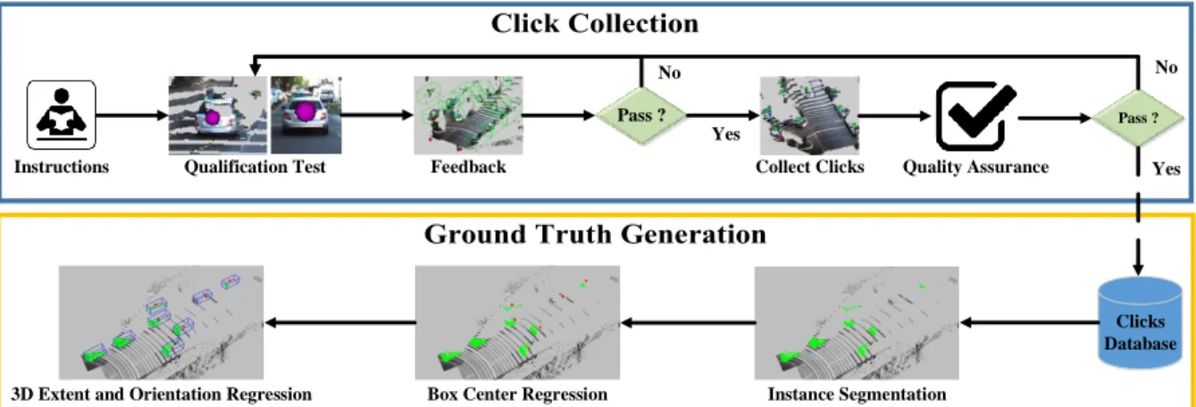
Figure 3.1: Overview of 3D Data Labelling Procedure

Figure3.1 provides an overview of the labelling or annotation scheme. The first stage consists of collecting click annotations with a custom labelling tool. A click is a singular 3D point that is obtained from annotators and indicates the presence of an object instance.

(34)

The annotators are trained with a qualification test that provides feedback on click accuracy and recall. Once the annotators pass the test, they are permitted to begin the annotation of the dataset. Quality assurance tests are randomly injected during click labeling to monitor the ongoing performance of the annotators. If the quality drops below a threshold, the annotator’s permission is revoked, and must re-qualify to continue. The collected clicks are stored into a central database for processing in the second stage.

The second stage uses the clicks to generate subsets of pointclouds that represent an object instance. The sample pointcloud is further processed through a deep neural network to obtain instance-level object segmentation followed by 3D bounding box estimates. The final output is a 3D bounding box and an instance segmentation mask for every collected click.

The remainder of this Chapter expands on the first and second stages of our labelling approach, starting with click collection in Section3.1, followed by the ground truth gener-ation method in Section3.2.

3.1 Click Collection

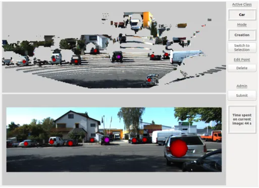
Click collection is performed in 3D space with a user interface visible in Figure3.2. Anno-tators are presented with a 3D and colorized point cloud, which is generated by running depth completion [21] on the LIDAR pointcloud. Annotators are then asked to click on all instances that belong to a single class. The annotators are restricted to labelling a single class to harness their knowledge of the scene to find all object class instances and to mini-mize task switching. Scenes are presented in temporal sequence to allow the user to carry knowledge of the previous scene over to the next, which eases the task of annotation. As the focus is solely on 3D labels, the clicks are only collected in 3D space. This requirement forces the annotator to be fully aware of the structure of the objects and that the click has been properly placed on each object. In cases of poor visibility, such as heavily shaded areas, the object’s structure will still be distinguishable in the 3D space. The camera sensor view of the scene is also provided to the annotators to help them locate the object instances.

3.1.1 Annotator Training

To maintain high-quality results, annotators must be trained before collecting clicks. They are initially provided with a set of instructions on how to properly perform the 3D

(35)

anno-Figure 3.2: The labelling GUI used by annotators to provide click labels for each object in the scene. The red points indicate points that are placed in the scene. The purple point signifies the current selection by the user. The right side of the GUI contains buttons for deletion, selection and submission of annotations.

tation task. Additionally, the annotators must go through a training sequence comprising of 5 test scenes. All of the test scenes are previously labelled such that the annotator’s attempts can be evaluated to provide performance analysis. The annotators are required to achieve a minimum threshold of recall and precision per scene. In addition, this task must be done under a time constraint, relative to the number of objects in the scene. The allowable time for a single test scene is computed as Tmax =N ×Tobject+Tscene, whereN is the number of objects in the scene, Tobject is the time allocated for clicking each object and Tscene is the time allocated to initially scan and understand the whole scene. Both

Tobject and Tscene are set to 7 seconds. When the annotators complete the annotation of these 5 scenes, they are provided with a review window which can be seen in Figure 3.3.

The review window displays each of the annotated scenes, and indicates the position of the annotations as well as the ground truth bounding boxes of objects in the scene. Clicks that are located inside ground truth bounding boxes are displayed in green, while those that

(36)

Figure 3.3: The annotator assessment window depicts the annotators correct and erroneous attempts. Thegreenbounding boxes with thegreenpoints indicate a proper annotation at-tempt. Thered bounding boxes are missed object instances. Thered point is an erroneous attempt that is not near to any of the correct instances.

are outside the boxes are displayed in red. Statistics pertaining to recall, precision, and the time taken to annotate the scene are also provided for the annotator. The annotator must attain a recall of 0.8, a precision of 0.6, and complete all scenes within the allocated time to pass the training. Otherwise, another set of five scenes is provided and the annotator must attempt a new training sequence. Annotators can repeat training as needed until they pass, allowing for simultaneous training and ability validation. This removes the need for the explicit annotator qualification test that is usually present in state-of-the-art methods [32,31].

3.1.2 Quality Assurance

To maintain accurate results during the annotation process, one test scene is injected in each batch at a random location. This test scene is pre-labelled and thus can be used to

(37)

detect a drop in the quality of annotations. Annotators are unaware of the existence of these scenes and are tested on the same passing criteria as in annotator training. If the annotator fails, the labels in the batch are discarded and the annotator must retake training to continue. If the annotator passes, the annotations in the batch are committed to the click database and a new batch begins seamlessly. This methodology diminishes the likelihood that new labels are saved when a particular annotator’s performance deteriorates.

Another approach to quality assurance is to collect clicks from multiple annotators for each scene. This allows additional processing of the results at the cost of multiple labelling. The added benefit of having multiple sources of annotation is that it allows more robust post-processing methods. A voting mechanism can be added such that clicks with agreement within a group or cluster of clicks are kept for further steps, while clicks that are outside of such clusters can be rejected. Additionally, the final single location of the click for an object instance can be represented by averaging the points within a cluster.

3.2 Ground Truth Generation

After click annotations have been collected and stored in a click database, a deep neural network is designed to perform instance-level object segmentation followed by 3D bounding box estimation. The model is based on the state-of-the-art F-PointNet [34], as outlined in Section 2.4.3. The proposed model contains three submodules, an instance segmentation network, a centroid regression network, and a bounding box estimation network that are run in succession, as illustrated in Figure 3.4. The submodules are preceded by a data pre-processing step which involves the production of the input to the overall network. The input to the network is a set of sub-sampled points near the collected clicks. The instance segmentation module removes background points using a mask generated from the likelihood of it belonging to the object in question. The centroid regression network takes the remaining object instance points as the input to estimate the object’s bounding box centroid. The final subnetwork, which is the bounding box estimation network, takes the 3D points and the estimated box centroid and outputs the final object bounding box that is parameterized by its centroid position, height, width, length and orientation. The following subsections describe each of the components of the ground truth generation in more detail.

(38)

3.2.1 Click Dataset Pre-processing

The purpose of the pre-processing step is to prepare the input data Pclk for the overall network from the dataset and annotation clicks.

The input is generated as a set of 3D points, with a size of N, that is contained in a K ×K ×K 3D volume centered at the click provided by the annotator, where K is a class-specific scale parameter. The points are centered around the click by subtracting the click coordinate from every point coordinate. A set of sampled points is thereby generated for every click recorded in the database.

The procedure differs if the model is being trained. For training, the set of points are generated using random click simulation from the KITTI 3D object detection dataset. A random point is selected from the points within a ground truth 3D bounding box. This random selection of points aims to replicate the annotator’s click selection during the labelling procedure. The output set of 3D points is sampled using a cubic volume centered at the selected random click. Five randomly-generated clicks are used to generate training data for each instance. This random selection serves as data augmentation to provide additional training data.

3.2.2 3D Point Instance Segmentation

The segmentation variant of PointNet [33] is used to perform instance level segmentation onPclk. The network is required to classify each point in Pclk with a label that indicates whether it belongs to an object or the background. Table 3.1 describes the architecture used for the instance segmentation module. Outputs from the conv3 and conv5 layers are extracted for the feature concatenation layer. Class information is also appended along with the local and global features. The parameterkis the number of classes and is encoded as a one-hot vector. The class information is obtained from the click database, where each click is associated with a class.

The output of the segmentation network is an N ×2 sized matrix, where the sec-ond dimension represents object and background class. The matrix is processed as a

N-dimensional binary vector to create a mask for the input. Masking Pclk generates a set of points with size M, where M ≤ N, that only contains the object points. During this process, the background points are filtered fromPclk. Finally, the masked points are normalized by its centroidCmask to generate the object pointcloud Pobj. This is done such that the set of points inPobj does not vary too much in bias.

(39)

Layer Kernel Weights Output conv1 1×1 64 n×64 conv2 1×1 64 n×64 conv3 1×1 64 n×64 conv4 1×1 128 n×128 conv5 1×1 1024 n×1024 maxpool - - 1×1024 concat - - n×(1024+64+k) conv6 1×1 512 n×512 conv7 1×1 256 n×256 conv8 1×1 128 n×128 conv9 1×1 128 n×128 conv10 1×1 2 n×2

Table 3.1: Instance Segmentation PointNet Layers

3.2.3 Center Regression

The object pointcloud is provided as an input to a 3D spatial T-Net, as described in Section

2.4.2. The output of the T-Net is a 3-d vector that represents the offset of the center of

a bounding box ∆Ct−net with respect to the origin of Cmask. The center regression is accomplished in a similar fashion to the residual centroid estimation of F-PointNet [34]. The object pointcloud is then normalized by Pobj − (Cmask + ∆Ct−net) to generate the bounding box pointcloud, Pbox. The bounding box pointcloud is used as the input for bounding box estimation. Table 3.2 lists the layers used for the center regression T-Net. Like the instance segmentation network, the class vector is appended in the concat layer.

3.2.4 3D Bounding Box Estimation

The classification variant of PointNet is used for bounding box estimation, but the final layers are replaced with regression output. The bounding box extent estimation follows the discrete-continuous loss definition described in Section 2.4.3. The model employs four templates (two for car, one for cyclists and one for pedestrians) based on the mean size of each object class from the training data split. Unlike traditional 3D object detectors [22] where every template is regressed and pruned via non-maximum suppression, the following model generates one best solution for each instance. This is done by classifying which

(40)

Layer Kernel Weights Output conv1 1×1 (3×128) n×128 conv2 1×1 (128×256) n×256 conv3 1×1 (256×512) n×512 maxpool - - 1×512 concat - - 1×(512+k) fc1 - 256 256 fc2 - 128 128 fc3 - 3 3

Table 3.2: Center Regression T-Net Layers

template best fits given input Pbox and then regressing the offset in height, width, length, and orientation from that template. During the training stage for the 3D box regression network, ground truth templates are chosen as those that have the greatest 3D IOU with the ground truth 3D bounding box.

The final output size of the bounding box regression layer is 3+4N S+2N H, as depicted in Table3.3. N Sis the number of templates, andN H is the number of heading bins. Three parameters for size and one parameter for classification are required for bounding box estimation. Similarly, a single parameter for heading bin and another single parameter for heading offset is regressed for orientation. The additional three parameters are for residual offset ∆Cof f to be applied to the center regression. The additional offset from the bounding box estimation network uses a different feature set to produce the correction from the initial estimation. The final center of the generated bounding box is formulated asCbox=Cmask + ∆Ct−net+ ∆Cof f.

3.2.5 Data Augmentation

During the training of the networks, data augmentation is added to the sampled pointcloud to reduce overfitting. The input points, Pclk, are jittered to add variation to the input data. The random noise is added to each of the points of the pointcloud with a normal distribution with a mean of 0 and standard deviation of 0.1. Additionally, the input points are randomly shuffled to vary the combination sequence of input points. This forces the network to avoid memorizing any specific pattern from the individual sequence and instead focus on the geometric shape of the object to learn hierarchical features, as this

(41)

Layer Kernel Weights Output conv1 1×1 128 n×128 conv2 1×1 128 n×128 conv3 1×1 256 n×256 conv4 1×1 512 n×512 maxpool - - 1×512 concat - - 1×(512+k) fc1 - 512 512 fc2 - 256 256 fc3 - 3 + 4NS + 2NH 3 + 4NS + 2NH

Table 3.3: 3D Bounding Box Regression PointNet Layers

shape remains present in the jittered examples. Random flip augmentations used in [20] are also applied in the following model to further augment the training data.

3.2.6 Network Training

Cross-entropy loss is used as the output of each point to train the instance segmentation network. The smooth L1 (Huber) loss is used as the loss function for centroid and bounding box regression, as described in Section2.3.6. For all the networks, the Adam optimizer [18] is used with an initial learning rate of 0.01 and an exponential learning schedule that decays the initial learning rate by 0.7 every 12,500 iterations. Dropout is used for regularization at 0.7 keep probability, and early stopping is used to choose the best model weights. All other parameters are kept as in the default implementation provided in the PointNet Architecture[33].

3.3 Conclusion

The proposed method utilizes the advantages of powerful human generalization capability and object detection networks to optimize the ground truth generation procedure. The use of spatial cues to assist the model to automatically generate accurate boxes and masks aims to reduce the tasks that must be undertaken by humans in the labelling effort. In the next Chapter, both quantitative and qualitative analysis of the proposed method is presented. The effectiveness and quality of the proposed method are demonstrated by

(42)

labelling an existing dataset. Finally, the method is applied to a novel dataset collected with the Autonomoose, the University of Waterloo self-driving vehicle testbed.

(43)

Click Database Click Dataset Pre-processing Center Regression T-Net

3D Bounding Box Size Regression Pointcloud Normalization MultiBin Angle Regression Segmentation PointNet Pointcloud Masking Instance Segmentation Center Regression

3D Bounding Box Estimation (PointNet) Residual Offset Regression Instance Level Segmentation Masks Pointcloud Pointcloud sampling near Clicks

3D Box Size (L, W, H) 3D Box Orientation 3D Box Center (x, y, z)

(44)

Chapter 4 Experimental Results

In the chapter, the performance of this study’s annotation scheme is evaluated. The analysis focuses on the evaluation of annotation time and the qualitative performance of the generated annotations. The KITTI object detection dataset is used as example of that which is to be labelled. The training-validation split of [2] is used, resulting in a 1:1 ratio for training and validation sets. All the neural network training is performed on the 3,712 frames from the training set, while the annotation procedure is tested on the 3,769 scenes of the validation set.

The annotation method’s generalization capabilities are also demonstrated by testing it on 300 frames of data collected from the University of Waterloo autonomous vehicle data collection platform, which is referred to as the Autonomoose dataset. The datasets differ in terms of location and the quality of pointcloud data because of the use of different Velodyne LIDAR sensors, depicted in Table4.1. The difference in the quality of the LIDAR is a property that serves as an effective test for generalization. The differing cities have differing distributions of car sizes and pedestrian representation between the datasets; these are additional properties that test for generalization.

Dataset Velodyne Model Frames Car Pedestrian Cyclist City

KITTI (VAL) HDL-64E 3712 Y Y Y Karlsruhe

Autonomoose VLP-32 300 Y Y N Waterloo

Table 4.1: KITTI 3D Object Validation Dataset vs. Autonomoose Dataset

(45)

label the KITTI Validation set. Each volunteer was taught to annotate based on the train-ing scheme mentioned in Section 3.1.1. The annotators were only permitted to progress with the actual labelling procedure if they passed the training. It is important to note that the frame sequences for KITTI were randomized due to the original design of the dataset. The annotations for Autonomoose dataset were collected by a small number of highly-trained annotators to obtain results for maximized efficiency. Autonomoose data was ordered sequentially during annotation to minimize annotator cognitive load.

4.1 Labelling Statistics

4.1.1 Annotation Time

In total, 58,832 seconds (16.34 hours) were required to annotate all 15,996 car instances in the 3,769 frames from the KITTI validation set. The car class was used exclusively because other classes comprised a very low percentage of the validation data. Annotating the 300 frames collected with the Autonomoose required 6,954 seconds (just under two hours) for 1,152 car and 138 pedestrian labels.

The proposed annotation scheme required around 3.7 seconds to annotate a single bounding box on the KITTI dataset and around 6 seconds to annotate a single bounding box on our data. The sole 3D object annotation times that have been pushlished [38] took roughly 114 seconds per instance, which is 19× longer than our approach. Generating annotations on our data took around 1.3 additional seconds per label on average, when compared to KITTI annotation by the same labeller. This can be attributed to the lower-quality LIDAR and camera images provided by our data when compared to the KITTI dataset, which required annotators to spend more time searching for all object instances in the scene.

However, the average time does not fully capture the efficiency of our annotation scheme. Figure 4.1 depicts a plot of the annotation time per object vs. the number of instances in the scene. Annotators tended to spend less time per object as the number of objects in the scene increased for both KITTI and Autonomoose data. This implies that annotation speed increases as the time spent observing the scene increases, which suggests that our approach can be quite efficient for multi-object label generation.

(46)

0 2 4 6 8 10

# Objects Per Frame

0 2 4 6 8 10

Annotation Time Per Object (Seconds)

Autonomoose Data KITTI Data

Figure 4.1: Annotation time per object (in seconds) vs the number of objects in the scene plots for annotating the KITTI validation set and Autonomoose data using the proposed annotation scheme.

4.1.2 Annotation Precision and Recall

The goal of the annotations is to maximize the performance of the trained model by pro-viding a pointcloud with a precise area. Thus, additional statistics that must be analyzed include precision, recall and accuracy. True positive (TP) is considered as having a click in the ground truth (GT) bounding box from the KITTI dataset. A missed GT box cor-responds to a false negative (FN). For cases where there are multiple clicks on a single vehicle, all the points are considered to be duplicates and are counted as false positives (FP). Clicks that are not in any GT boxes are categorized as FP. For evaluation, the orig-inal 3D GT boxes are inflated by a factor of 1.5 to allow a larger area to be considered as positive. Pinpoint accuracy is not necessary because the network can perform well in producing the final bounding box so long as the click lies in the close vicinity of the object. Ground truth bounding boxes without any points in KITTI datasets are filtered out for

3D Ground Truth Generation Using Pre-Trained Deep Neural Networks