SN applied sciences [online], 1, article ID 1412. Available from: https://doi.org/10.1007/s42452-019-1433-0
Data stream mining: methods and challenges for
handling concept drift.
WARES, S., ISAACS, J. and ELYAN, E.
2019
SN Applied Sciences (2019) 1:1412 | https://doi.org/10.1007/s42452-019-1433-0
Data stream mining: methods and challenges for handling concept
drift
Scott Wares1 · John Isaacs1 · Eyad Elyan1 © The Author(s) 2019 OPEN
Abstract
Mining and analysing streaming data is crucial for many applications, and this area of research has gained extensive attention over the past decade. However, there are several inherent problems that continue to challenge the hardware and the state-of-the art algorithmic solutions. Examples of such problems include the unbound size, varying speed and unknown data characteristics of arriving instances from a data stream. The aim of this research is to portray key challenges faced by algorithmic solutions for stream mining, particularly focusing on the prevalent issue of concept drift. A compre-hensive discussion of concept drift and its inherent data challenges in the context of stream mining is presented, as is a critical, in-depth review of relevant literature. Current issues with the evaluative procedure for concept drift detectors is also explored, highlighting problems such as a lack of established base datasets and the impact of temporal dependence on concept drift detection. By exposing gaps in the current literature, this study suggests recommendations for future research which should aid in the progression of stream mining and concept drift detection algorithms.
Keywords Stream · Data · Mining · Concept drift
1 Introduction
The global datasphere is a notional environment in which data produced worldwide is contained. According to Rein-sel et al. [62], the global datasphere contained over 20 ZB of data (20 billion TB) in 2017. Its growth is expected to continue rapidly, and by 2025 it is hypothesised to contain 160 ZB of data. Such exponential growth is due, in part, to hardware developments and an increase in user avail-ability and accessibility.
Data is now generated at a near constant and limitless rate, resulting from an array of devices, networks and eve-ryday tasks such as credit card transactions and mobile phones [1]. Data arriving online and in a sequential, con-tinuous fashion is known as a data stream. These data streams provide a potential source of valuable quantita-tive and qualitaquantita-tive data, providing it can be extracted in a timely manner.
Adapted machine learning techniques can be used to harvest interesting information from the stream in a process known as stream mining. However, the volume, velocity and temporal nature of the arriving data can cause complex challenges for stream mining. Unlike stationary data in traditional batch learning scenarios, streaming data can be looked at only once and is unbound in size. This is an inherent problem for streaming data and poses a chal-lenge for real time processing.
Concept drift is another inherent problem, caused by streaming data changing, or evolving, over time. Concept drift also occurs at varying rates of severity. A shift in the underlying distribution can result in the feature vectors of arriving instances no longer reflecting the class label. This causes a negative impact upon the reliability and accu-racy of classifiers that make predictions using the current distribution.
Received: 10 July 2019 / Accepted: 9 October 2019
* Scott Wares, [email protected]; John Isaacs, [email protected]; Eyad Elyan, [email protected] | 1The Sir Ian Wood Building, Robert Gordon University, Garthdee Road, Aberdeen, Scotland, UK.
This paper provides a critical review of stream mining with a focus on stream mining challenges, concept drift detection algorithms and problems with their evaluative process such as a lack of established datasets. This research is primarily concerned with supervised data stream min-ing and drift detection methods. Literature and techniques involving unsupervised approaches, such as Sethi and Kantardzic [64] and de Mello et al. [23], are not reviewed. Unlike existing reviews such as Gama et al. [36], this paper reviews modern, recent approaches to handling concept drift, as well as established methods covered in earlier reviews. Ditzler et al. [26] provides a summary of the chal-lenges and approaches for learning in both static and evolving data streams. However, their review lacks detail and depth in their explanation of techniques and instead. Similarly, the recent review by Krawczyk et al. [48] primarily focuses on ensemble methods, and only briefly highlights the most popular non-ensemble based techniques. The timeliness of this review is of particular interest. Success-ful mining of data streams can potentially provide rich quantitative and qualitative information. Such informa-tion could have a tremendous impact on business prac-tices across various industries, such as oil and gas where streaming data is abundant. However, because of the chal-lenges posed by stream mining it is relatively unharnessed. This research suggests that the reason for stream mining not be fully harnessed is that the domain of concept drift detection is not progressing at a quick enough pace. For example, the domain of imbalanced data, in the context of stream mining, has produced various adaptations for algorithms to handle class imbalance, such as DDM-OCI [69], LFR [67], Learn++.NIE [24] and Learn++.CDS [25]. The field of class imbalance in stream mining has also pub-lished recent reviews that provide timely suggestions for future research [47], whereas in contrast the reviews for concept drift are several years old [36] and do not encap-sulate recent advancements.
The main contributions of this paper are outlined as follows:
1. Critically and extensively review existing literature, dis-cussing both well established and recent concept drift detection techniques.
2. Categorise existing methods for concept drift detec-tion based on their underlying model. Existing meth-ods are categorised as either statistical based, window based or ensemble based.
3. Identify and discuss clear gaps in the literature areas for improvement, particularly relating to current evalu-ative measures and the availability of public datasets for benchmarking.
4. Provide possible avenues for future research that address current research gaps in the existing literature.
This paper is structured as follows. Section 2 provides a general overview of stream mining, its key differences from traditional batch learning and design requirements for stream mining algorithms. Section 3 focuses on con-cept drift, providing definitions and discussing algorithmic requirements. Section 4 categorises and critically reviews existing concept drift detection techniques. Section 5
discusses evaluation methods, as well as highlighting the concept of temporal dependence. Section 6 concludes the paper and offers suggestion for future research direction.
2 Stream mining overview
Data streams posess specific and unique characteristics that differentiate them from other forms of data. In tradi-tional machine learning contexts, the data is often referred to as “batch” data. That is, all of the data is immediately available in its entirety and is stored in memory. This is of stark contrast to stream mining, where data streams produce elements in a sequential, continuous fashion, and may also be impermanent, or transient, in nature [2,
33]. This means stream data may only be available for a short time. The difference between traditional methods and data streams is described by Babcock et al. [2] in the following ways:
1. Data elements in the stream arrive online.
2. The system has no control over the order in which data elements arrive to be processed, either within a data stream or across data streams.
3. Data streams are potentially unbound in size.
4. Once an element from a data stream has been pro-cessed, it is discarded or archived. It cannot be retrieved easily unless it is explicitly stored in memory, which is small relative to the size of data streams.
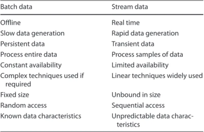
The unique characteristics of a data stream contribute to the challenges in processing its arriving elements. Since batch data is persistent, it can be queried once in its entirety and individual data elements can be accessed at random. Data streams however, since transient, must be queried continuously by the algorithm. The data elements in the stream cannot be accessed at random; they can only be accessed in the sequence in which they arrive from the stream. The key differences between processing traditional batch data and stream data are shown Table 1.
Data streams are either static (sometimes referred to as stationary) or evolving, and are classified depending on the condition of their core distribution.
Static data has an underlying distribution that does not shift over time. That is, the features that define the target label for learning remain constant and consistent. Static
datasets are frequent in traditional machine learning con-texts where features defining ground truth labels do not change [18].
Unlike static data, the distribution for an evolving data stream may change over time. Feature vectors may change over a time period t such that they no longer reflect the class label. Aggarwal [1] describes how data streams pos-sess an inherent temporal component that causes them to be time dependent by nature. Consider customer purchas-ing behaviour as an example. A model trained to predict weekly sales for a clothing store might use attributes such as advertising costs, promotions and customer footfall. However, this model may become less accurate over time, perhaps due to seasonality. The shift in distribution over time is commonly known as concept drift.
In the domain of machine learning, traditional appli-cations implement batch learning techniques on static datasets. Batch learning approaches involve having the entirety of the training data available at any given time. The data can be processed once or multiple times before an algorithm produces an output decision.
Data streams by nature are incompatible to batch learn-ing for a number of reasons. Most obviously where tradi-tional applications have all of the data available immedi-ately, data streams must be mined in a distributed fashion since examples arrive continuously and in a sequential manner. In contrast to batch and multi-pass learning, stream mining algorithms must be designed to work with one pass of the data only [1].
A solution to the ineffectiveness of batch learning may at first seem obvious; translate batch learning algorithms into one-pass variants. However, the innate temporal nature of data streams may render this solution redun-dant as a one-pass conversion approach may not consider the evolution of the underlying distribution. Concept drift is something stream mining algorithms simply must take into consideration.
Since data streams are unbound in size, the volume and velocity can result in the imposition of hardware limita-tions. The most obvious of which is memory; it is not fea-sible to continuously explicitly store stream elements since their maximum size is almost always unknown. A second hardware limitation is processing resource. The speed at which elements arrive from a stream, as well as the stream size, can quickly consume available resources. As such, stream mining algorithms should be both computation-ally fast and lightweight [18].
3
Concept drift
Traditional machine learning algorithms operate with the assumption that the data distribution is static. For data streams, the distribution of arriving examples may change over time due to the stream’s innate temporal nature. This renders traditional batch learning algorithms unsuitable for applications that learn from data streams.
In reality, data streams produce copious amounts of data at a near constant rate. Gama [33] provides examples of such streams, including surveillance systems, sensor networks and telecommunication systems. However, with recent modern hardware developments these streams are produced by new devices such as smart household appli-ances and car navigation systems. Algorithms that seek to learn from data streams must be able to accurately model the underlying distribution. The ability to detect and adapt to changes in the distribution of examples is paramount for data stream mining algorithms.
The shift in the underlying distribution of examples arriving from a data stream is referred to as concept drift. Concept drift occurs over time and the rate at which the drifts occurs varies. It can be responsible for various symp-toms, including previous examples to become irrelevant; their distribution no longer accurately reflects their cor-responding class label. This is reflected in the clothing store sales prediction example previously mentioned. If seasonality causes clothing sales to be higher in the sum-mer months, then examples from winter months may not accurately reflect class labels. It may be the case that the model predicts low sales, but due to seasonality there are less people shopping and the sales are in fact high for a winter season. As such, models must be capable of forget-ting previous examples once concept drift has occurred.
3.1 Definition
A learning algorithm observing examples with a sta-tionary distribution would observe training examples in the form (𝐱i,yi) , where 𝐱i is the feature vector and
yi𝜖{c1,c2,…,cn} for the ith example. A class prediction Table 1 Batch data versus streaming data
Batch data Stream data
Offline Real time
Slow data generation Rapid data generation Persistent data Transient data
Process entire data Process samples of data Constant availability Limited availability Complex techniques used if
required
Linear techniques widely used Fixed size Unbound in size
Random access Sequential access
Known data characteristics Unpredictable data charac-teristics
at a particular time stamp t would be given as ŷt based on the feature vector 𝐱t.
In contrast, a data stream may produce examples with a non-stationary distribution. The stream may initially consist of examples ei = (𝐱i,yi) , similar to that of a static distribution. However, if the distribution should shift at some point in time then this may no longer hold true. According to Gama et al. [36], concept drift between time t0 and t1 can be defined as:
where pt is the joint distribution at time t between the feature vector 𝐱i and the target class label yi.
Kelly et al. [45] states that concept drift may occur in three distinct ways. Firstly, the class prior probabilities
p(y) may change over time. Secondly, the class distri-butions p(𝐱∣y) may change over time. And thirdly the class posterior distribution p(y∣𝐱) may change. From the point of view of classification, only p(𝐱∣y) changes would affect the prediction and therefore require an algorithmic response.
The rate at which concept drift occurs can be catego-rised as one of three distinct forms; sudden drifts, grad-ual drifts and recurring drifts. Brzezinski and Stefanow-ski [15] concisely describes these three types of concept drift; sudden drifts occur when the source distribution is suddenly replaced by another distribution entirely, gradual drift occur at a much slower rate, and recurring drifts occur when older concepts reappear after some time period. Drifts can also be described as incremental where the drift consists of many intermediate changes, for example a network sensor deteriorates and becomes less accurate [36].
Similarly to categorising the rate of change, concept drift itself can be defined as either real or virtual [36,
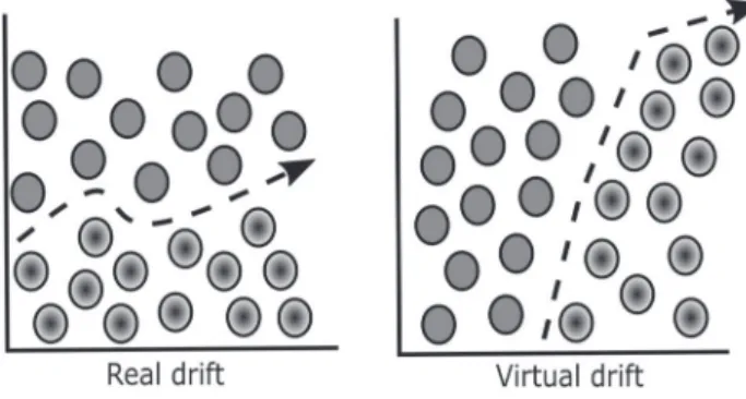
71, 74]. Real concept drift refers to changes in p(y∣𝐱) , a change in the probability of a class label y given feature vector 𝐱 . This can result in classifier decision boundaries becoming affected. Alternatively, virtual drift refers to changes in p(𝐱) but not in p(y∣𝐱) . The result in this case is that the distribution has changed but the decision bound-aries of the classifier are unaffected. Figure 1 illustrates the differences between real and virtual drift.
As is described by Zliobaite [74], it is not important if the drift is real or virtual since p(y∣𝐱) is dependant on
p(𝐱∣y) . Explicit characterisation of various types of con-cept drift is effectively illustrated by Webb et al. [70]. This paper will not make any further differentiation between real or virtual drifts.
Where stream mining algorithms bring with them their own set of challenging algorithmic requirements, algorithms (1)
pt0(𝐱i,yi)≠pt1(𝐱i,yi),
for concept drift detection must also meet certain demands. The following points are considered to be critical challenges that concept drift detection algorithms should overcome [35, 36]:
1. Detect as soon as possible the point at which the dis-tribution has changed.
2. The crossover period during a shift in concept can pro-duce noise. For example as distribution D0 shifts to D1 , examples produced by D0 will act as noise for D1. 3. Algorithms should be computationally faster than the
arrival time of examples from the stream. They should also be lightweight enough to not consume more than some fixed amount of memory for storage.
Any classifier operating with stream data must contain mechanisms to meet these requirements, otherwise their predictive performance will diminish over time. The predic-tive model will likely have to be capable of updating with new data as it arrives, or even replacing itself entirely.
4 Concept drift detection
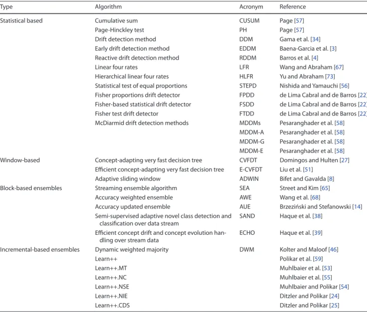
This section critically reviews existing concept drift detec-tion techniques by categorising drift detecdetec-tion methods as either statistical based, window based or ensemble based. Table 2 provides a full illustration of the categorisation and techniques covered by this paper.
4.1 Statistical methods
The Sequential Probability Ratio Test (SPRT) [66] is the back-bone to a number of algorithms for concept drift detection. Given two distributions P0 and P1 for time period w, should the underlying distribution shift from P0 to P1 then the prob-ability of observing elements from P1 should be higher than
the probability of observing elements from P0 . The statistical test is given as:
Introduced by Page [57], the Cumulative Sum (CUSUM) is a statistical technique based on the SPRT and is commonly adopted for concept drift detection. It receives as an input the residual of any filter, for example a Kalman filter, and outputs an alarm when the mean of the input data differs greatly from zero. Bifet [7] gives CUSUM as
(2) Tn w =log P(xw…xn∣P1) P(xw…xn∣P0) = n ∑ i=w logP1[xi] P0[xi] =Tn−1 w +logPP1[xn] 0[xn]
where 𝜖t is the current observed value, v is the allowed magnitude of change, t is the current time and h is a parameter defined threshold. This expressions functions for detecting changes that occur in a positive direction. If changes in a negative direction are required for detection then the min() function should be used in place of max().
CUSUM is memoryless in the sense that the probability of a drift being detected is not related to a drift having already been detected. It is also worth noting that the accuracy of CUSUM is dependant on the parameters v and (3)
g0=0
gt =max(0,gt−1+𝜖t−v)
ifgt >hthen alarm andgt =0, Table 2 Summary of concept drift detection techniques
Type Algorithm Acronym Reference
Statistical based Cumulative sum CUSUM Page [57]
Page-Hinckley test PH Page [57]
Drift detection method DDM Gama et al. [34] Early drift detection method EDDM Baena-Garcia et al. [3] Reactive drift detection method RDDM Barros et al. [4]
Linear four rates LFR Wang and Abraham [67]
Hierarchical linear four rates HLFR Yu and Abraham [73] Statistical test of equal proportions STEPD Nishida and Yamauchi [56] Fisher proportions drift detector FPDD de Lima Cabral and de Barros [22] Fisher-based statistical drift detector FSDD de Lima Cabral and de Barros [22] Fisher test drift detector FTDD de Lima Cabral and de Barros [22] McDiarmid drift detection methods MDDMs Pesaranghader et al. [58]
MDDM-A Pesaranghader et al. [58] MDDM-G Pesaranghader et al. [58] MDDM-E Pesaranghader et al. [58] Window-based Concept-adapting very fast decision tree CVFDT Domingos and Hulten [27]
Efficient concept-adapting very fast decision tree E-CVFDT Liu et al. [51] Adaptive sliding window ADWIN Bifet and Gavalda [8] Block-based ensembles Streaming ensemble algorithm SEA Street and Kim [65]
Accuracy weighted ensemble AWE Wang et al. [68]
Accuracy updated ensemble AUE Brzeziński and Stefanowski [14] Semi-supervised adaptive novel class detection and
classification over data stream
SAND Haque et al. [38] Efficient concept drift and concept evolution
han-dling over stream data
ECHO Haque et al. [39] Incremental-based ensembles Dynamic weighted majority DWM Kolter and Maloof [46]
Learn++ Polikar et al. [59]
Learn++.MT Muhlbaier et al. [53]
Learn++.NC Muhlbaier et al. [55]
Learn++.NSE Muhlbaier and Polikar [54]
Learn++.NIE Ditzler and Polikar [24]
h. Low values of v enable faster detection rates but at the cost of an increased rate in false positives.
The Page-Hinckley (PH) test, also proposed by Page [57], is a variant of the previously mentioned CUSUM test. The PH test can detect changes in the average behaviour of a process. The PH test for an increasing signal can be given as [7]:
where 𝜖t is the current observed value, v is the allowed magnitude of change, t is the current time and h is a parameter defined threshold. If the signal is decreasing then Gt =max(gt,Gt−1) and Gt−gt >h should be utilised as the stopping rule instead. Similarly to CUSUM, the PH test is memoryless but its accuracy is again parameter dependent on the values of v and h. Larger values of h will result in a lower false alarm rate, but some changes may also be missed altogether.
While the two algorithms are similar, they do offer solu-tions for different data streaming scenarios. Since CUSUM uses the residual from any predictor as an input is well suited for various applications of stream mining, and has been recently used for anomaly detection in video streams by Yang et al. [72]. PH is instead ideally suited for detecting abrupt changes in signal processing environments, but has also been adopted recently for the development of a rule learning algorithm for regression [29].
The performance of drift detection algorithms based on SPRT is often reliant on their false alarm and missed detection rates, as noted by Gama et al. [36]. However, during evaluative procedures such measures are usually overlooked as metrics to evaluate drift detector perfor-mance. This is explained fully in Sect. 5 of this research. The primary drawback and impact on performance is both algorithms’ reliance on the parameters v and h. Both CUSUM and Page-Hinckley are considered state-of-the-art drift detectors in this category.
Another statistical method for detecting concept drift is based around monitoring the class distribution’s con-stancy over time, as described by Brzezinski and Stefanow-ski [15]. This is undertaken by adopting various statistical techniques that produce “alarms” when the class distribu-tion begins to change as time passes.
Drift Detection Method (DDM) [34] is a method that sta-tistically compares two windows and controls the errors produced by a learning model during prediction. One win-dow contains all of the data, and the second winwin-dow con-sists of only data from the start of the stream to the point
(4)
g0=0
gt =gt−1+ (𝜖t−v) Gt=min(gt,Gt−1)
ifgt−Gt >hthen alarm andgt=0,
at which the error rate of the prediction model increases. The windows are not kept in memory, only statistical infor-mation and recent errors are stored.
It is assumed that the error rate will decrease as the number of examples for observation increases, so long as the distribution is stationary. It is therefore suggested that a significant increase in the error rate of some learn-ing model would indicate a change in the class distribu-tion. DDM involves two principle variables in the form of
pt and st , where p is the probability of misclassification, s
is the standard deviation and t is some timestamp. The standard deviation st is given as st =√pt(1−pt)∕t . When
pt+st reaches its minimum value the following conditions
are checked:
• pt+st ≥pmin+2⋅smin as a warning level. Examples are
stored in preparation of contextual drift.
• pt+st ≥pmin+3⋅smin as drift level. Concept drift is
assumed to exist, the learning model is reset and a new model is trained using examples stored since the warn-ing level was triggered. pmin and smin are also reset. DDM is almost memoryless, only statistics pt and st are stored alongside the necessity of some available memory to store examples for retraining. A major flaw with DDM is that is only suitable for the detection of abrupt drifts. Gradual drifts can cause examples to be stored in memory for lengthy time periods which has the potential to cause catastrophic memory overflows.
A number of algorithms have built upon DDM and have aimed to improve its performance. The most famous of these is the Early Drift Detection Method (EDDM) [3]. EDDM uses the same approach and heuristics as DDM, however, rather than monitoring error rates, the distances between errors is measured. As predictions improve, the distance between two misclassification errors should increase. The window resizing follows the same proce-dure as DDM. The fundamental drawback to EDDM is that at least 30 errors are required for calculation which causes issues when applying this to imbalanced datasets. A more modern proposal to improve DDM is that of Bar-ros et al. [4], who suggest the Reactive Drift Detection Method (RDDM) which discards older instances of par-ticularly gradually occurring drifts in order to overcome potential memory overflows.
The DDM-OCI algorithm [69] was developed to solve the problem with using EDDM and imbalanced datasets. DDM-OCI makes the assumption that for imbalanced data-sets, drifts only occur when there is a change in the minor-ity class recall during classification. However it is entirely possible that a drift can occur without affecting the minor-ity class recall, for example a drift from data that has an unbalanced class distribution to one which is balanced.
DDM-OCI also suffers from an issue where a number of false positives can be triggered due to a weakness in its test statistic R̂t
TPR.
With DDM-OCI falling short of overcoming the class imbalance problems present in EDDM, the Linear Four Rates framework (LFR), was proposed by Wang and Abra-ham [67]. It is designed as a direct improvement over the DDM-OCI algorithm. LFR monitors the four values, or rates, given by a typical confusion matrix; precision and recall for both minority and majority classes. Statistical bounds are set as thresholds and should any of the four rates exceed the threshold then a drift is assumed to have occurred.
The current, most recent advancement in these algo-rithms is the Hierarchical Linear Four Rates method (HLFR) proposed by Yu and Abraham [73], given in Algorithm 1. HLFR operates using a two layer, hierarchical structure wherein the first layer is responsible for detecting potential drifts, and the second layer validates said drift and com-municates this information back to the first layer. Layer one monitors the same four rates of the confusion matrix as was introduced by LFR. When a drift is detected, layer two applies a permutation test to confirm if the detected drift is true or a false positive. In the occurrence of a false positive the testing process restarts.
Experimental results using real datasets indicate that HLFR outperforms DDM, EDDM and LFR in terms of not only accuracy but also in terms of its time to detection (detection delay). The framework presented with HLFR symbolises a move away from the traditional “concept drift detector plus classifier” approach. This current method suf-fers from various evaluation problems, discussed in depth in Sect. 5. The proposed framework of HLFR is a concrete starting point for future research that aims to address such issues.
DDM and EDDM are considered state-of-the-art statisti-cal based detectors [7], even though they have drawbacks in relation to imbalanced data. Algorithms that have aimed to address this, such as DDM-OCI and LFR have fallen short. The result of which is that two, aged drift detectors that are sub-par in terms of performance are still considered
state-of-the-art. A second reason is due to the datasets used in concept drift experimentation. This is explained fully in Sect. 5, but a lack of benchmark datasets means that many experiments used simulated data in which parameters can be defined to avoid class imbalance, thus artificially avoiding the drawbacks of DDM and EDDM.
STEPD [56], or Statistical Test of Equal Proportions, mon-itors the predictions of a base classifier for drift detection in a similar manner to that of DDM and EDDM. However, STEPD also uses two parameters as significance levels to distinguish between detected drifts and warnings. These are 𝛼d=0.003 and 𝛼w =0.05 respectively. STEPD uses two windows to compare the result of the classifier. The first window is a “recent” window, of which its size if defined by a parameter with a default value of 30 instances. The second window is the “older” window which contains all instances observed since the last detected drift. STEPD compares the accuracies of these windows through a hypothesis test of equal proportions, given as
where ro is the number of correct predictions from exam-ples within the no “older window”, rr is the correct predic-tions from examples within the nr “recent” window and
̂
P= (ro+rr)∕(no+nr) . The result is used to calculate the
p-value from the standard normal distribution table and is then compared against to 𝛼d and 𝛼w to determine if a drift or warning alarm must be issued. If p-value < 𝛼d then a drift is detected, similarly if p-value < 𝛼w then a warning is signalled.
The authors recognised that for small sample sizes the statistical test of equal proportions was ineffective, admit-ting that Fisher’s Exact test [32] should have been used but was ignored due to its high computational cost. Recent work by de Lima Cabral and de Barros [22] proposes three new methods using the Fisher’s Exact test, Fisher Propor-tions Drift Detector (FPDD), Fisher-based Statistical Drift Detectors (FSDD) and Fisher Test Drift Detector (FTDD). All three methods use the same approach as STEPD in regards to the two windows and the significance thresh-olds. However, these approaches use different statistical tests and measure the difference in errors rather than cor-rect predictions.
FPDD uses the Fisher’s Exact test when the number of errors or correct predictions in either window is smaller than five, otherwise it operates exactly like STEPD. FSDD extends FPDD such that instead of using the test of equal proportions in situations where the number of errors or correct predictions in either window is smaller than five, the chi-square test for homogeneity of proportions is (5)
T(ro,rr,no,nr) = |ro∕√no−rr∕nr|−0.5× (1∕no+1∕nr)
̂
applied [17] FTDD explicitly uses the Fisher’s Exact test for drift detection. Experimental results showed that all three proposed methods outperformed STEPD, with very little difference between themselves.
The McDiarmid Drift Detection Methods (MDDMs) proposed by Pesaranghader et al. [58] uses a weighting scheme to give substance to elements of a sliding win-dow to enable faster concept drift detection. MDDM applied McDiarmid’s inequality [52] to detect drifts in evolving streams. The algorithms uses a sliding window of size n which stores prediction results. If the prediction is correct, a 1 is inserted into the window, otherwise a 0 is inserted. Each element in the window is weighted such that wi<wi+1 . This means that elements at the head of the window have larger weights than that of the tail. Three methods based on different weighting schemes are pre-sented. MDDM-A which uses the arithmetic weighting scheme, MDDM-G which uses the geometric weighting scheme and MDDM-E which uses the Euler weighting scheme. The arithmetic weighting scheme for MDDM-A is given as
where d≥0 is the difference between two consecutive weights. The geometric scheme used by MDDM-G is given as
where r≥1 is the ratio of two consecutive weights. Finally, the Euler scheme adopted for MDDM-E is given by the authors as
where 𝜆≥0 . Prediction results are processed sequen-tially and the weighted average of all elements within the window is calculated alongside each arriving prediction result. This is used to update two variables, 𝜇wt the current weighted average and 𝜇mw the maximum weighted average observed thus far. A drift is detected if there is a significant difference between 𝜇wm and 𝜇tw . The significance is deter-mined by McDiarmid’s inequality. The authors selected popular concept drift datasets for experimental testing, including Elec2, Forest Covertype and Poker Hand. These (6) wi =1+ (i−1) ×d (7) wi =r(i−1) (8) r=e𝜆
are explained in Sect. 5 of this paper. Their results found that MDDMs outperformed existing methods including EDDM, CUSUM and Page-Hinckley in terms of drift detec-tion delay and classificadetec-tion accuracy.
4.2 Window-based detectors
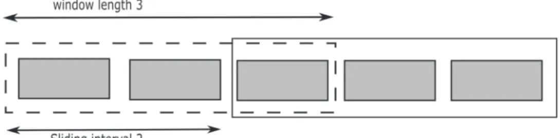
Concept drift detection algorithms that are window-based operate in a unique way. Rather than monitoring arriving instances from a stream individually, sliding windows of varying sizes, widths, are instead statistically monitored. Larger windows correlate with higher performance accu-racy, however they may also contain concept drift within themselves that could escape unnoticed. Smaller windows tend to facilitate better concept drift detection. The sizing of a window is a fundamental problem when designing any stream mining algorithm that utilises sliding windows. Figure 2 provides an illustration of how a sliding window operates.
The Hoeffding Tree is a mathematically justified algo-rithm used to construct decision trees. The Very Fast Deci-sion Tree (VFDT) is a heuristic algorithm proposed by Domingos and Hulten [27] that is based on the Hoeffding Tree. The VFDT is an algorithm which incrementally con-structs a decision tree of incoming examples from a data stream, without the need to store examples in memory. A critical difference between the Hoeffding tree and tra-ditional classification trees lies in the selection of which node is used for splitting. Where traditional trees adopt techniques such as Information Gain [60] to determine the best node for splitting, VFDTs use the Hoeffding bound to determine how many examples are necessary to identify the best splitting node based on a user defined confidence threshold. The Hoeffding bound states that, for a random variable r in range R and where ̄r is the mean of n observa-tions, with probability 1−𝛿 the true mean is at least r̄−𝜖 where 𝜖 is given as
It is also worth noting that the Hoeffding bound has been suggested to be statistically inappropriate for constructing (9)
𝜖=
√
R2ln(1∕𝛿)
2n
Fig. 2 Sliding window. Borders identify two different windows
decision trees for data stream mining [21, 44, 63]. VFDTs are, however, only suitable for static streams and include no method for forgetting or restarting learning in the pres-ence of concept drift. In order to enable VFDTs to account for concept drift, Hulten et al. [41] introduced Concept-adapting Very Fast Decision Tree (CVFDT). CVFDT monitors a sliding window of examples. As new examples arrive, CVFDT updates its node statistics by incrementing counts of the new, arriving, examples. Counts that relate to the oldest example in the window, which must be forgot-ten, are decremented. If necessary, older examples are removed from the window. Hulten et al. [41] states that if the concept is changing then nodes that previously passed the Hoeffding test may no longer pass. In this case, CVFDT grows a second sub-tree with the new best attribute, according to the Hoeffding bound, at its root. If the new sub-tree’s accuracy outperforms that of the older tree then it replaces it completely.
Criticising CVFDT for not offering mechanisms which handle specific types of drift, such as gradual or abrupt, Liu et al. [51] proposed the E-CVFDT algorithm which utilises a caching mechanism. Their results show that E-CVFDT yields a higher classification accuracy for grad-ual concept drifts, but does not make any improvements during sudden drifts.
The Adaptive Sliding Window (ADWIN) algorithm [8] is another popular, window-based detector for coping with concept drift. Assuming a stream of examples x1,x2,…,xn , produced by some distribution at time t, these serve as inputs to ADWIN to produce sliding window W. Let 𝜇̂w denote the average of examples contained within W and
𝜇w represent the unknown average of 𝜇t such that t∈W .
Let n be the length of W and n0 and n1 be the lengths of
W0 and W1 respectively, such that n=n0+n1 . Algorithm 2
provides the algorithm for ADWIN.
Whenever two “large enough” subwindows of W dis-play “distinct enough” averages, a drift is assumed to have occurred, and the older of the two subwindows is dropped. The terms “large enough” and “distinct enough” are defined by the Hoeffding bound statistic. The average
of the two subwindows are tested to determine if they are larger than 𝜖cut , given as |𝜇w0−𝜇w1|>2𝜖cut where
This was considered computationally expensive since all “large enough” subwindows are checked for potential cuts. The window contents are also explicitly stored and mem-ory requirements scale linearly with the window size. This has the obvious drawback of potentially large memory and processing requirements.
A solution to the resource demands of ADWIN is pro-posed in the form of ADWIN2, provided in Algorithm 3.
In order to reduce the computational time when deter-mining the best cutting point in the window, buckets are adopted as a means for grouping data within the window. Such buckets have two core elements; capacity and con-tent. Each time a new example arrives from the stream, if the element is “1” then a new bucket is created of content
1 and capacity equal to the number of elements arrived since the last observed “1”. The remaining buckets are then compressed.
In order to eliminate the problems of high memory demands caused by the explicit storing of all window con-tents, a variation of the exponential histogram [20] is used. The performance of ADWIN2 is given by the authors in Big O notation as O(logW) memory and cutpoints, with the worst case per example equating to O(log2W).
ADWIN2 is usually referred to directly as ADWIN in pub-lished work and is considered one of the state-of-the-art concept drift detectors. A common problem with sliding windows is that the width usually needs to be predefined. Varying the width of the window has an impact on per-formance, thus applying the correct width value is impor-tant. Typically this is done by means of some user-defined
(10) m= 1∕n 1 0+1∕n1 𝛿′= 𝛿 n 𝜖cut= √ 1 2m⋅ln 4𝛿′
parameter. ADWIN, however, is parameterless and the slid-ing window is sized dynamically by the algorithm itself. It also provides excellent performance due to the use of buckets and the adaptation of the exponential histogram to for compression.
4.3 Block-based ensemble detectors
In machine learning, an ensemble refers to a group or col-lection of classifiers that work together to achieve greater predictive performance. Block-based ensembles process data in blocks, or chunks, of some specified size. The per-formance of block-based ensemble methods is based heavily on the chunk size. Similarly to that of sliding win-dows, larger chunks tend to produce more accurate clas-sifiers but may contain concept drift within themselves. Alternatively, smaller based chunk sizes are typically more effective at drift detection but produce inferior perform-ing classifiers.
The Streaming Ensemble Algorithm (SEA) was first pro-posed by Street and Kim [65] and is a block-based ensem-ble learning algorithm. Individual classifiers are constructed from examples read in sequential blocks (chunks), which are then added to a fixed size ensemble. If the ensemble is full, then the worst performing classifier is removed from the ensemble entirely.
In their experiments, C4.5 [61] classifiers are used for building the ensemble. The output prediction is given as the simple majority voting of the entire ensemble. Results for testing with concept drift showed that the algorithm was capable of recovering quickly by discarding classifiers trained on the outdated data.
A notable drawback to SEA is the way in which classifiers are replaced. Merely replacing the worst performing classi-fier with the most recently trained has the potential to still leave several, outdated and poorly performing classifiers in the ensemble, depending on the predetermined ensemble size.
This is improved upon by Wang et al. [68]’s Accuracy Weighted Ensemble (AWE), a block-based algorithm which trains a new learning model with each new chunk of data in a similar fashion to that of SEA. Where AWE improves upon SEA is in the model replacement. AWE uses a version of the mean square error to select n best classifiers to construct an entirely new ensemble, thus removing all other outdated and poorly performing classifiers. The algorithm for AWE is given in Algorithm 4.
Let S denote a data stream in chunks S1,S2,…,Sn where each chunk is of equal size and Ci represent some classifier for Si . The weight of classifier Ci is the estimated prediction error using the most recent data Sn . Since Sn is a data stream and will produce examples in the form (𝐱,c) where 𝐱 is the feature vector and c is the class label, the classification error of Ci is 1−fci(x) where fci(x) is the probability that x is an example of class c. As such, the mean square error of Ci is given by
Should a classifier predict randomly then the mean square error can be given as:
A random classifier contains no meaningful knowledge of the data, it makes predictions simply at random. Therefore
MSEr is used as a threshold for weighting and classifiers
whose error rate is at least equal to MSEr are discarded. The weight of a classifier Ci is given as:
One drawback to AWE is the issue of chunk-size optimisa-tion, however it should be noted that this is common in all block-based ensemble methods. A second drawback is the weighting function of AWE, in particular the MSEr threshold. In environments with sudden concept drift it can have a silencing effect on the entire ensemble result-ing in no class prediction [14].
Brzeziński and Stefanowski [14] proposed the Accuracy Updated Ensemble (AUE) algorithm as an improvement to that of AWE. The algorithm for AUE is given in Algorithm 5.
(11) MSEi= S1 n ∑ (x,c)∈Sn ( 1−fi c(x) )2 (12) MSEr = ∑ c p(c)(1−p(c))2 (13) wi =MSEr−MSEi
AUE implements online classifiers enabling the indi-vidual learning models to be updated directly rather than only adjusting weights as per AWE. If no concept drift were to occur between a series of chunks then the classifiers would improve as if they were trained on one large chunk. This means the block size can be reduced without risking the performance accuracy of the ensemble classifiers. The weighting function in AUE is a simplified version of that used in AWE, and is given as
where MSEi is calculated identically as it is in AWE and 𝜖 is a small constant value to allow weighting calculations when
MSEi is equal to 0.
Experimental results showed that AUE performed more accurately than AWE on all similar datasets apart from one where the performance accuracy was equal. A second implementation of this algorithm, AUE2, was suggested by Brzezinski and Stefanowski [15] which improves on the memory usage and accuracy of AUE by implementing a new weighting function and pruning base learners.
AUE overcomes the problems present in AWE. The weighting function is redesign to cope with sudden con-cept drifts, and the use of online classifiers allows smaller chunk sizes to be used without a severe reduction in classi-fier accuracy. However when no concept drift is occurring, all classifiers are updated with arriving chunks. Should this continue over multiple chunks then the outcome is that ensemble classifiers lose their uniqueness.
Recent advances in concept drift detection using block-based ensembles have introduced new algorithms entirely. The Semi-supervised Adaptive Novel Class Detec-tion and ClassificaDetec-tion over Data Stream (SAND) framework is proposed by Haque et al. [38]. SAND consists of four (14)
wi = MSE1 i+𝜖,
independent modules; Classification, Novel Class Detec-tion, Change Detection and Update.
The framework maintains an ensemble of classifiers based on k-nearest neighbour, using algorithms such as k-means. The ensemble is initially trained on some training data. When an instance arrives from some stream it is clas-sified using majority voting. It also produces a confidence value which indicates the ensemble’s confidence in the prediction. These confidence values are stored in a sliding window.
The Change Detection module monitors the distribu-tion of confidence values within the sliding window. Any significant change in the distribution is assumed to be caused by the existence of concept drift. Once change has been detected, a new chunk of data is used to update the ensemble and the chunk boundaries are determined dynamically. Updating is undertaken by requesting only class labels for instances in the current chunk where the confidence values were weak. The ensemble is then updated with the new model and the sliding window is reset.
Experimental results showed that SAND was capable of achieving good prediction accuracy using limited labelled data, however its execution time was inefficient due to the high resource cost of the Change Detection module being executed after the calculation of individual confidence scores.
In order to attempt to remedy the poor execution time of SAND, the Efficient Concept Drift and Concept Evolu-tion Handling over Stream Data (ECHO) was proposed by Haque et al. [39]. ECHO operates in the same manner as SAND, however, the execution of the Change Detection module is selective rather than at each calculation of the confidence threshold. Two methods of selectively invoking the Change Detection module. The first is to use a fixed
threshold 𝛾 , such as the classifier confidence threshold. If the confidence of a test instance Cx is less than 𝛾 , the Change Detection module is invoked. The second pro-posed approach is to calculate the probability of invoca-tion based on the Cx . A high confidence value would result in a low probability of invocation.
ECHO performs competitively and is suitable for use in environments which generate a low level of labelled data. However, in stream mining there is an innate assump-tion that class labels are always available with arriving instances. Whilst this may not be the case in real world scenarios, since concept drift detection is still in its infancy it follows that this assumption can continue to be made. Classifiers are only updated by labels for which there was a low confidence value. While this does aid in situations where labels are missing by lowering the demand for labels, there is no existing mechanism for actually deter-mining if a label is available or not. The result is that classi-fiers may not be updated with information when there is an available class label, which will negatively impact the potential performance of the ensemble.
4.4 Incremental ensemble detectors
Incremental, or online, ensembles are another method of ensemble based learning. In contrast to block-based ensembles, incremental ensembles process elements sequentially rather than in chunks.
Dynamic Weighted Majority (DWM) was first proposed by Kolter and Maloof [46]. DWM is an ensemble of classi-fiers referred to as ’experts’, where each is given an asso-ciated weight. For some test example, the experts each provide a prediction. This is then used in combination with their weights to output the overall prediction in the form of the class which has the largest accumulated weight total.
Should an individual expert provide an incorrect pre-diction, then its corresponding weight is reduced. If the output prediction of DWM is incorrect then a new expert is created and is assigned a weighting of 1. Experts are nor-malised by uniform scaling such that the highest weight-ing possible is 1. Experts with a weight lower than a user-defined threshold value are removed. Through the use of uniform weights and incremental learning, the authors state that the DWM algorithm is capable of handling con-cept drift.
DWM is considered one of the state-of-the-art concept drift detection methods, and has been as a benchmark algorithm in recent studies reviewing concept drift [7,
36, 76]. However, one particular problem with DWM is the way in which experts are added. Rather than adding
a new expert when the ensemble prediction is incorrect, the age of experts and historical prediction accuracy could be taken into consideration. The base learner also explicitly maintains examples in memory which has the potential to consume large amounts of resources, depending on the stream size. Other algorithms such as CVFDT and ADWIN have already solved this issue so it follows that similar implementations could be made to DWM.
4.4.1 Learn++ algorithms
The Learn++ algorithm family is a set of algorithms con-sisting of an ensemble of incrementally trained classifi-ers using batches of data and weighted majority voting. According to Liao et al. [50] existing algorithms in the Learn++ family include Learn++, Learn++.NC, Learn++. MT, Learn++.NSE, Learn++.NIE and Learn++.CDS. Elwell and Polikar [31] also mention the Learn++.MF algorithm as part of the family.
The original Learn++ algorithm, suggested by Polikar et al. [59], constructs k classifiers for a single batch of incoming data. Examples from this batch are used to train a single, first classifier. Prediction errors are used to produce a weighted distribution of all examples, with misclassified examples possessing a higher probability of being sampled. Training the second classifier through to the k classifier for the ensemble, training examples are selected based on the weighted distribution of all exam-ples. Classification errors are then used to update the weighted distribution.
One problem with Learn++ is that all base classifiers are persisted over time T, resulting in old data never being for-gotten by the ensemble. This can cause a problem known as ’outvoting’. Older classifiers in the ensemble may pro-duce incorrect predictions due to the aged examples they are trained on. If the outdated classifiers make up the majority of the ensemble, even if their weights are small, they can ’outvote’ the classifiers trained on newer data. Thus through the majority weighted voting procedure, produce incorrect predictions. Another problem is that without forgetting old information, concept drift cannot be accounted for.
Older algorithms in the Learn++ family sought to pro-vide solutions to the concept drift problem. Learn++.MT [53] solves the outvoting problem by using a dynamic weighted voting technqiue. Learn++.NC (New Class), proposed by Muhlbaier et al. [55], furthers this concept and introduces a Dynamically Weighted Consult and Vote (DW-CAV) mechanism which enables incremental learning of new classes. Learn++.NC enabled base classi-fiers within the ensemble to consult among themselves
when classifying a given example, and weights the deci-sion of each base classifier. Classifiers check their predic-tions against classes which they are trained and, based on the decision of other classifiers, check if their pre-diction is in-line with others. If a classifier’s decision is an outlier compared to the majority, the classifier may either reduce it’s voting weighting or withdraw from pre-dicting altogether. These algorithms, however, are only suitable for static, stationary, environments where the distribution does not change.
Learn++.NSE, proposed by Muhlbaier and Polikar [54], aims to account for various forms of concept drift. An ensemble of classifiers is trained on the current data dis-tribution D at time t. Change is monitored by examining the performance of the ensemble over time. Learn++. NSE will generate a new classifier and combine it with the ensemble when the prediction error of the current ensemble falls below some threshold. Classifiers are weighted according to the time t they were instantiated, such that newer classifiers have a larger weighting than older classifiers during prediction.
Whilst Learn++.NSE aimed to address the issue of evolving data, none of the existing Learn++ algorithms accounted for class imbalance at this stage. Learn++.NIE [24] extends Learn++.NSE, but incorporates evaluation measures for data class imbalance, such as f-measure. Learn++.NIE also implements sub-ensembles in place of individual classifiers in order to reduce stochastic errors. An alternative approach was proposed by Ditzler and Polikar [25], whose Learn++.CDS algorithm instead uses preprocessing with SMOTE, an oversampling method, rather than changing the evaluation metric to account for class imbalance. SMOTE adds instances to the minor-ity class in order to create a more balanced dataset.
The comparative performance of the Learn++ algo-rithms was reviewed by Liao et al. [50]. The performance of each algorithm is dependent heavily on the base clas-sifier used. This was especially apparent in environments with imbalanced data and incremental learning. The cur-rent state of the Learn++ algorithm family requires con-siderable work to produce solutions that can cope with concept drift and imbalanced data, although discussion of the latter is out of scope for this research. Learn++. NSE provides a starting point for using the Learn++ fam-ily for concept drift detection. However it is outdated and its approach weighting favours newly created clas-sifiers during prediction which is a flawed approach; it is entirely feasible that older classifiers in an ensemble may be better equipped to make predictions than newer classifiers.
5
Evaluation
In traditional machine learning scenarios, the typical evaluation procedure is to train a model, cross-validate and then test using metrics such as prediction accuracy or f-score. For stream mining this approach is ineffec-tive. Since stream data arrives online in a continuous and sequential fashion, it is not possible to first train the model and then test. Instead one of two methods can be used; prequential evaluation, sometimes referred to as inter-leaved-test-then-train, or holdout evaluation.
Prequential evaluation is implemented using the fol-lowing procedure. For each arriving element from a stream the model is first tested by predicting the class label, after which the same element is used to train the model. Pre-quential evaluation can be used in conjuction with sliding windows and decaying factors to improve classification results in evolving data streams. A full comparative assess-ment is given by Gama et al. [35].
The holdout evaluation procedure offers an alternative approach. This involves with-holding a subset of data exam-ples from the classifier to be used as a training set at specific time intervals, for example every one hundred thousand instances. Algorithm 6, adapted from Bifet and Kirkby [9], shows an example algorithm for holdout evaluation. The most obvious problem for holdout is the acquisition of examples for use as training data. A solution to this is to sys-tematically store arriving samples from the stream at vary-ing intervals. Similarly, ascertainvary-ing the adequate number of examples to provide accurate evaluation measurements also poses a challenge. It is suggested by Bifet and Kirkby [9] that a test set in the region of tens of thousands of examples is sufficient, however, this is an enormous potential range and doesn’t provide a concise estimate.
Krempl et al. [49] states that a problem with evaluating stream mining classifiers in general is a lack of benchmark datasets for cross comparison. Instead, datasets are often synthesised used tools such as MOA [10]. This is also a problem for evaluating concept drift detection algorithms.
Few benchmark datasets exist for testing concept drift detectors. The most popular dataset used for evaluat-ing concept drift detection algorithms is the Electricity Dataset [40]. This dataset is used in various concept drift related research publications [7, 34, 46, 75]. This dataset was taken from the Australian New South Wales electric-ity market, in which electricelectric-ity prices are not statically set. Instead, the price fluctuates according to demand. The dataset is constructed of 45,312 electricity prices which were taken at 30 min intervals. Examples are labelled as either “UP” or “DOWN” which reflect their current price in comparison to the last 24 h. Another popular dataset is the Forest Covertype [13] dataset. This consists of 581,012 instances of 54 attributes that describe various types of forest cover of the Roosevelt National Forest in northern Colorado. The KDD’99 dataset is well known and subject to somewhat extreme temporal dependence. This dataset contains information pertaining to simulated intrusions in a military network environment. It contains 23 class labels representing either normal traffic or some form of intrusion. The dataset contains over 494,000 records of 41 features each. This dataset is of considerable age, but due to the high level of temporal dependence has been used in recent studies such as Zliobaite et al. [76]. The Poker Hand dataset from UCI Machine Learning Repository [28] contains one million records of 11 attributes that repre-sent a poker hand of five cards from a standard 52 card deck. Each card has two corresponding attributes, the suit and the rank, and there is one additional attribute that describes the hand, e.g. royal flush or full house. A dataset similar to Poker Hand that contained more class labels was used in the work of Cattral et al. [16]. The Airlines dataset from Data Expo 2009 [42] contains 120 million records of 13 attributes relating to flight departure and arrival information from internal commercial flights in the USA between October 1987 and April 2008. The target class label is the arrival delay given in seconds, and the classifi-cation goal is to determine the flight delay time given the arrival and departure information. This dataset has been used in the work of Ikonomovska et al. [43].
Another fundamental problem in evaluating drift detectors stems from the use of classifier accuracy as an
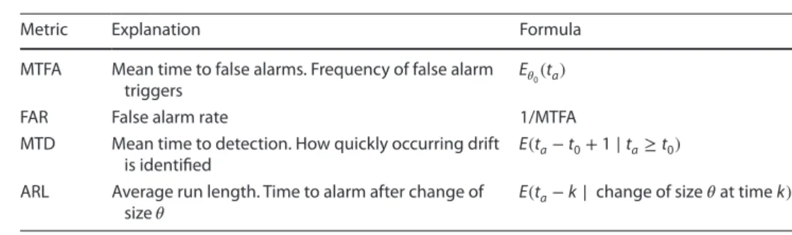
evaluation metric. This has been criticised in recent litera-ture [7, 12, 76] where it has been suggested that classifier accuracy doesn’t reflect the performance of the concept drift detector. Bifet [7] explains that drift detectors should be evaluated in terms of their ability to handle false alarms, their true detection rate and the time taken to correctly identify an occuring drift. This is reflected in evaluation criteria proposed by Basseville et al. [5] and Gustafsson and Gustafsson [37], which are given in Table 3. These are existing, historic metrics which capture properties of con-cept drift detectors, however, at the time of writing there appears only the work of Bifet et al. [11] utilises these met-rics for evaluation.
These metrics have existed for over a decade, yet are not used in published work. One possible reason for this is a lack of frameworks which support these metrics. Each must be independently calculated when implementing models, which is time consuming and can increase com-plexity. Since prediction accuracy is readily available in vir-tually all machine learning frameworks, it’s of no surprise that this metric is used to evaluate the impact of change detectors. This is only bolstered by the idea that in most instances the performance of the change detector itself may be viewed as unimportant; only the performance of the classifier truly matters.
The lack of an existing evaluation framework was an issue that was addressed by Bifet et al. [11] where the authors propose CD-MOA, a GUI extension to MOA (Mas-sive Online Analysis). CD-MOA offers an interface for evaluating change detectors. However, the evaluation measures provided are again different. CD-MOA provides information on time and memory resources, as well as a metric called RAM-Hours which merges both time and memory together. The most recent version of CD-MOA also provides a measure based on Cohen’s Kappa statistic [19], which compares observed accuracy with an expected accuracy.
A further issue with the metrics of Basseville et al. [5] and Gustafsson and Gustafsson [37], as given in Table 3, is their numerousness. Having five independent statisti-cal measures to evaluate a drift detector obfuscates a true representation of performance. In order to tackle this,
Table 3 Drift detector
evaluation metrics Metric Explanation Formula
MTFA Mean time to false alarms. Frequency of false alarm triggers
E𝜃0(ta)
FAR False alarm rate 1/MTFA
MTD Mean time to detection. How quickly occurring drift is identified
E(ta−t0+1∣ta≥t0)
ARL Average run length. Time to alarm after change of size 𝜃
Bifet [7] proposed a new single metric, the Mean Time Ratio (MTR), which encapsulates the ratio between MTFA and MTD metrics. The motivation of this was that the MTFA and MTD metrics are arguably the two most important, thus providing a single metric representing these elimi-nates the confusion of having five metrics. The MTR metric is given as follows.
Ultimately, the problem with current evaluation metrics is a lack of agreement and absence of gold-standard tech-niques. The metrics presented in Table 3 represent perfor-mance characteristics of a change detector, but numer-ousness and a lack of frameworks has left them virtually unused. The MTR metric aims to eliminate the problem of numerousness by providing a single metric which com-bines both the mean time to false alarms and the mean time to detection. CD-MOA provides a framework for evaluation, but provides a different set of metrics within its GUI for evaluating drift detectors. The result is that drift detectors are evaluated based on their impact to classifier accuracy, however this doesn’t truly evaluate the concept drift detector itself. Further research should aim to estab-lish a standardised set of statistical evaluation metrics that encapsulate the various performance characteristics of a drift detector, as well as its impact on classifier accuracy.
Existing statistical measures focus on the evaluation of baseline classifiers. The Kappa statistic proposed by Cohen [19] is a statistical measure for evaluating clas-sification results when using imbalanced data, both in the context of streaming data and in traditional batch learning. The Kappa statistic is defined as
where P is the accuracy of some base classifier and Pran is the accuracy of a classifier that predicts labels at random.
The Kappa statistic, however, is not a suitable metric when temporal dependence exists within the data, as shown by Zliobaite et al. [76]. Instead, the authors pro-pose a new statistic called Kappa Temporal, defined as
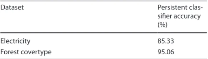
where Pper is the probability of a Persistent classifier, a classifier that simply predicts that the next class label will the same as the immediately previously known class label. Using this measure, trained classifiers performing correctly will achieve a kper score of 1, or if performing (15) MTR(𝜃) = MTFA MTD × (1−MDR) = ARL(0) ARL() × (1−MDR) (16) k= P−Pran 1−Pran, (17) kper= P−Pper 1−Pper,
worse than the Persistent classifier Pper , a score of 0. The substantial drawback to the Kappa Temporal measure is the direct inverse to the Cohen’s Kappa statistic described above. Kappa Temporal is ineffective for imbalanced data-sets since a Majority class classifier, a classifier that simply predicts the class with the largest prior probabilities, will outperform that of a Persistent classifier.
Zliobaite et al. [76] offer a solution to this problem by combining both Cohen’s Kappa statistic and the Kappa Temporal statistic together, forming the Combined Meas-ure [76]. This is given as
This Combined Measure will provide a statistical evalua-tion score of 0 if either the Kappa or the Kappa Temporal metrics fail. This provides a single evaluation metric that encapsulates a classifier’s ability to cope with both tempo-ral dependence and imbalanced data. However, it is only a statistical metric and does not offer any mechanism for base classifiers to handle temporal dependence during the classification process.
Further evidence of the need for additional evalua-tion criteria outwith of classifier performance is shown by Bifet [7]. A “No Change” detector is compared to state-of-the-art drift detectors using a Naive Bayes classifier with both the Electricity and Forest Covertype datasets. The No Change detector is a drift detector that performs no sta-tistical monitoring of the stream data but instead outputs a false positive change every 60 instances. The results of this show that the No Change detector outperforms state-of-the-art detectors in terms of accuracy on both datasets. This reinforces the concept that the use of accuracy as a metric for the performance of concept drift detectors is insufficient.
A possible direction for future research is to design and produce new statistical evaluation criteria. Krawc-zyk et al. [48] suggests that metrics such as memory con-sumption, update time and decision time of drift detectors should be taken into account for evaluation. New metrics should not focus solely on the predictive accuracy of the base classifier but incorporate performance factors of the drift detector. A potential start would be to find a suitable statistical combination to incorporate classifier accuracy with the metrics given in Table 3. This would provide a new, harmonious statistical measure that represents both the drift detector and classifier performance.
The work of Bifet [7] not only suggests that accuracy is a poor metric for evaluating drift detectors, but also that the existence of temporal dependence within data-sets that contain concept drift is the cause the false alarm phenomenon found with the superior performance of the No Change detector.
(18)
K+=√max(0,k)max(o,k