Computational Bayesian Methods for Insurance Premium Estimation

(1)

Computational Bayesian Methods for Insurance

Premium Estimation

Oscar Alberto Quijano Xacur

A Thesis

for The Department of

Mathematics and Statistics

Presented in Partial Fulfillment of the Requirements

for the Degree of Doctor of Philosophy (Mathematics) at

Concordia University

Montreal, Quebec, Canada

July 2019

c

(2)

CONCORDIA UNIVERSITY SCHOOL OF GRADUATE STUDIES

This is to certify that the thesis prepared

By: Oscar Alberto Quijano Xacur

Entitled: Computational Bayesian Methods for Insurance Premium Estimation

and submitted in partial fulfillment of the requirements for the degree of

Doctor Of Philosophy

complies with the regulations of the University and meets the accepted standards with respect to originality and quality.

Signed by the final examining committee:

Chair Mary Appezzato External Examiner Arthur Charpentier External to Program Dennis Kira Examiner M´elina Mailhot Examiner Yogendra P. Chaubey Thesis Supervisor Jos´e Garrido

Approved by Cody Hyndman

Chair of Department or Graduate Program Director

Andr´e G. Roy Dean of Faculty

(3)

Abstract

Computational Bayesian Methods for Insurance Premium Estimation Oscar Alberto Quijano Xacur, Ph.D.

Concordia University, 2019

Bayesian Inference is used to develop a credibility estimator and a method to compute insurance premium risk loadings. Algorithms to apply both methods to Generalized Linear Models (GLMs) are provided. We call our credibility estimator the entropic premium. It is a Bayesian point estimator that uses the relative entropy as the loss function. The risk measures Value-at-Risk (VaR) and Tail-Value-at-Risk (TVaR) are used to determine premium risk loadings. Our method considers the number of insureds and their durations as random variables. A distribution to model the duration of risks is introduced. We call it unifed, it has support on the interval (0,1), it is an exponential dispersion family and it can be used as the response distribution of a GLM.

(4)

Contribution from Authors

Bayesian Credibility for GLMs

Oscar Alberto Quijano Xacur Research, writing, editing and proof-reading. Jos´e Garrido Research supervisor, funding and proof-reading.

(5)

List of Figures

3.1 Good mixing example . . . 20

3.2 Bad mixing example . . . 21

3.3 Running means of two parallel chains . . . 22

3.4 Autocorrelation plots . . . 23

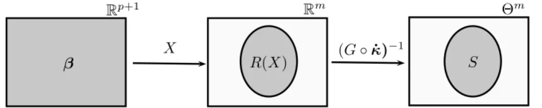
7.1 From left to right the grey zone represents the values thatβ, R(X) and S can take, respectively. . . 51

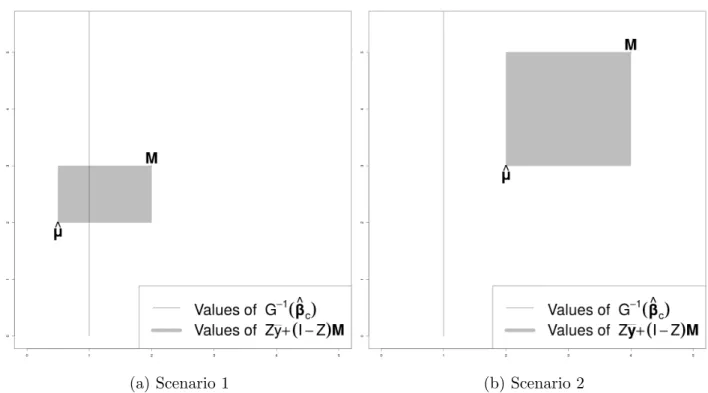
7.2 Values of the left and right hand side of (7.4) in both scenarios . . . 54

8.1 Residuals for frequency model . . . 72

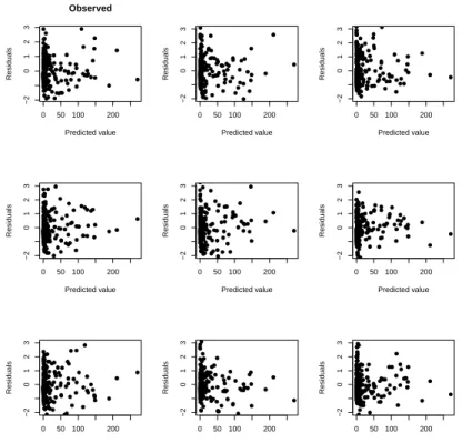
8.2 Comparison of observed residuals and replicated residuals . . . 73

8.3 Residuals for the number of zeros . . . 74

8.4 Entropic and frequentist frequency estimation comparison . . . 74

8.5 Residuals for severity model . . . 76

8.6 Entropic and frequentist severity estimation comparison . . . 77

9.1 Density of the unifed for different values of its mean µ . . . 80

9.2 Variance function of the Unifed . . . 82

9.3 Two histograms of exposure data from the insuranceData R package . . . 86

9.4 Beta fit for Singapore auto histogram . . . 87

9.5 Estimated posterior predictive distribution for Unifed and Beta distributions for Singapore auto exposures . . . 88

9.6 Residuals of Unifed GLM . . . 93

(10)

10.1 Test quantities for frequency model . . . 108

10.2 Test Quantities for the Severity Model . . . 109

10.3 Test Quantities for the Exposure Model . . . 110

10.4 Premiums that return the unearned premium . . . 119

10.5 Premiums for classes categorized by expected duration. . . 126

10.6 Comparison between the C(t, r) premium, the entropic premium and the ex-pected mean premium principle. . . 127

(11)

List of Tables

8.1 Deviance decomposition of some common EDF’s . . . 60

8.2 e(ϕ) for the three proper exponential dispersion families . . . 66

8.3 Vehicle insurance variables . . . 69

8.4 Frequency model. . . 70

8.5 Summary table of frequency model estimated coefficients . . . 71

8.6 Severity model. . . 75

8.7 Summary table of severity model estimated coefficients . . . 75

9.1 Float overflow of the Irwin-Hall implementation. . . 80

9.2 Summary of frequentist GLM . . . 92

9.3 Exposure Bayesian model . . . 94

9.4 Summary table of Bayesian exposure model estimated coefficients . . . 94

10.1 Simulated Homogeneous Policy Year Losses . . . 106

10.2 Loaded Premiums . . . 111

10.3 β∗ by premium type and category . . . 123

10.4 Total Collected Premiums . . . 124

(12)

List of Abbreviations

EDF Exponential Dispersion Family

GLM Generalized Linear Model

MCMC Markov Chain Monte Carlo

HMC Hamiltonian Monte Carlo

PRNG Pseudo Random Number Generator

PPD Posterior Predictive Distribution

SLLN Strong Law of Large Numbers

VaR Value at Risk

(13)

Notation

• Vectors, unless otherwise stated, are assumed to be column vectors.

• log(x) means natural logarithm of x.

• Given a positive measure m, it will be said that something is true modulo m, with notation [m], if it is true except on some set E with m(E) = 0.

• If µand ν are measures, we use µ_≪ν to express that µis absolutely continuous with respect to ν. When µ_≪ν and ν _≪µ we will write µ_≡ν and we will say that µand ν are equivalent.

• If (Ω,_F, m) is a measure space,L1_(Ω,_F_{, m) is the set of all the}_F_{-measurable functions}

such that

∫

|f(x)_|dm(x)<_∞.

When Ω and _F are clear from the context we useL1(m) instead of L1(Ω,_F, m).

• We use N to denote the natural numbers. It is assumed that they start at 1, i.e.

N=_{1,2, . . ._}.

• E and V are used for the expectation and variance of a random variable, while V is used to denote the variance function of an Exponential Dispersion Family.

• N(µ, σ2_)T_{(a, b) denotes the normal distribution with mean}_µ_{and variance}_σ2 _truncated

(14)

Chapter 1 Introduction

Insurance is a collective effort to mitigate the risk of some financial loss. The idea is for a group of individuals, theinsureds, to contribute some money, thepremium, into a fund called the reserve. The reserve is then used to pay for the losses incurred by the insureds. Thus, the money contributed by many pays for the losses of a few. This allows the premiums to be much lower than the potential loss.

The reserve is managed by an entity called the insurer. We refer to the set of insureds as the insurance portfolio or simply the portfolio. This thesis focuses on non-life insurance where the financial loss is about casualties that occur to a specific good or property (e.g. a car or a house). This object is referred to as the risk. The insurance conditions agreed upon by the insured and the insurer are expressed in a contract called the insurance policy

or simply the policy.

One can never be certain that the reserve will be enough to pay for all future losses. Thus, the fundamental question of insurance is: what should the premium be in order for the reserve to be likely to pay for all losses? We leave this concept vague for now. In Chapter 9 we make the phrase “likely to pay” more precise.

Assumptions about the insurance portfolio have to be made in order to answer the fun-damental question. In actuarial mathematics there is a set of assumptions that we consider to be a building block for the rest of the theory. These assumptions define what we call the

homoegenous portfolio.

(15)

random variables representing the future losses of each risk. We say that the portfolio is

homogeneous when the Si’s are independent, identically distributed and with finite mean.

New methods and ideas are usually first tested in the homogeneous portfolio and then generalized to more complex situations. We adhere to this practice along this work.

The Strong Law of Large Numbers (SLLN) gives us a starting point to look for premiums that result in solvent reserves. It tells us that with probability one

S1 +· · ·+Sn

n →µ,

where µ=E[S1]. Actuaries callµ the pure premium.

We now know that the pure premium is too low to obtain a solvent reserve. A classical paper that exemplifies the insufficiency of the pure premium is de Finetti (1939), where a gambler’s ruin setting based on de Moivre (1756) is used. In Chapter 9 we prove the insufficiency of the pure premium from a different viewpoint.

The premium should then be the pure premium plus some additional amount. We refer to this additional amount as the risk loading. Of course, there has been a lot of effort to determine how much should the risk loading be. Premium principles and risk measures have been used for this purpose (see for instance Young (2006) and Hardy (2006)).

The areas of study in actuarial mathematics presented so far propose models that assume some known underlying probability distribution or at least some known quantities about them like the mean or a quantile. When one wants to apply such models to a real problem it is necessary to estimate these quantities based on past data. Thus we enter in the realm of statistics.

The theory of statistics tells us that estimations based on few observations are not reliable. Credibility theory is the branch of actuarial mathematics that aims to solve the problem of estimating the pure premium when there are few observations. Chapter 1 gives an account of the existing methods and ideas in credibility theory.

An important extension of the homogeneous portfolio has been the relaxation of the iden-tically distributed part. Such portfolios are called heterogeneous. Different approaches have been proposed in the actuarial literature, but all of them (to the best of our knowledge) have a common factor: they start by dividing the portfolio into (approximately)

(16)

homoge-neous groups. This is known as segmenting the portfolio or simply segmentation. Nowadays Generalized Linear Models (GLMs) are widely used in practice for this purpose. They are introduced in Chapter 3.

The new contributions of this thesis are contained in Chapters 6, 7, 8 and 9.

Chapter 6 talks about linear credibility for GLMs. Linear estimators have played a central role in credibility theory. Exact linear credibility means choosing a prior whose posterior mean is a linear function of the sample average. Previously existing linear credibility results for GLM are not exact. The research for this thesis started with the search of a prior that would give linear credibility for GLMs. We ended up proving that such a prior does not exist, which is the main result of Chapter 6.

Chapter 7 introduces entropic credibility. It is a Bayesian point estimator that uses the relative entropy as loss function instead of the usual square error loss. The relative entropy and its properties are introduced in Chapter 4.

In Chapter 8 we present a new probability distribution: the unifed. It has support on (0,1) and it can be used as the response distribution of a GLM. We propose it for modelling the duration of policies in an insurance portfolio.

In Chapter 9 we propose methods to compute the premium risk loading using GLMs. Along this work Bayesian statistics are used for parameter estimation. Partly because it is a natural framework for credibility problems but also because we find the interpretation of Bayesian estimates more natural than the frequentist one. In Chapter 5 we give a brief introduction to Bayesian statistics and we discuss the differences of interpretation between the Bayesian and the frequentist approach. Markov Chain Monte Carlo (MCMC) algorithms are necessary for the application of all our results in any practical situation. They are introduced in Chapter 2.

We think of a model as a lens through which one looks at reality. In consequence, we see model assessment as a tool for understanding what aspects of reality are replicated reasonably well by a model and which ones are not. For this reason, when assessing the goodness of fit, we have deliberately avoided the use of asymptotic distributions that arise from the assumption that the chosen parametric family is the true one. We prefer the use of replicated samples, which we introduce in Chapter 6.

(17)

In the applied examples we focus on illustrating new concepts and algorithms and we have left cross-validation out of the examples. Nevertheless, we do recommend the use of cross-validation in any predictive modeling context where our proposed procedures are used. The examples given in Chapters 7, 8 and 9 were coded in R (R Core Team (2019)) and stan (Stan Development Team (2018)). We created an R package that can be used to reproduce the results of all our examples. It can be downloaded fromhttps://gitlab.com/ oquijano/mythesis.

(18)

Chapter 2 Credibility Theory

Usually the first step taken by insurers is to segment their portfolio into homogeneous classes. Then it proceeds to estimate the risk premium and loading for each class. The first essential problem in credibility theory can be formulated in this way: how many observations are needed in a class in order for such estimations to be reliable (in some sense)?

Assuming that we can answer this question, let us introduce some terminology. For those classes in which there is a large enough number of observations we say that the estimation is

credible or that we have full credibility. Otherwise we say that the estimation is not credible

or that we have partial credibility. Additionally, we will call criterion for full credibility or

full credibility criterion any method that aims to answer this question.

The second essential problem in credibility theory is: given a group for which we do not have sufficient policyholders for a fully credible estimation, how can we get a reliable estimation of the pure premium?

Following the development of credibility theory, we make the distinction between three different types of estimation.

We callcredibility estimator orcredibility premium the final estimation that we consider more reliable than the sample average ¯Sn.

We callempirical estimator orempirical premium, an estimator coming from a sample of the population of interest.

We call manual estimator or manual premium an out-of-sample estimator. Typically it comes from previous or out-of-sample experience of the same insurer with similar risks or

(19)

from pooled information from different insurers.

Traditionally, credibility estimators have been obtained by combining in some way em-pirical and manual estimators. We call credibility formula any expression involving the data and the manual estimator with the purpose of obtaining a credibility estimator.

2.1 Overview of Credibility Results

The historical development of credibility theory can be divided into two parts. On the one hand we have results concerning criteria for full credibility and on the other hand we have those that assume partial credibility and develop a credibility formula.

Early articles on full credibility criteria for the pure premium are Mowbray (1914) and Whitney (1918). Both of these papers develop models in the context of workers compensation. A well known paper with a more general scope is Perryman (1932). The criteria introduced in this paper depends on two parameters kandpwhich are interpreted as “the observed pure premium should be within 100k% of the expected pure premium with probabilityp”. In this sense, it is said that an estimation ˆµof µ is fully credible (k, p) if

P(_|µˆ₋µ_{| ≤}kµ)_≥p. (2.1)

By using the Central Limit Theorem, Perryman assumed that there were enough observations for ˆµ to be normally distributed and in this way he found for what minimum sample size (2.1) is satisfied. Mayerson et al. (1968) generalized Perryman’s work by dropping the as-sumption of normality for ˆµ. They did it in a distribution-free manner. Only some moments of the distribution are required. They achieved this using the Cornish-Fisher expansion. Many decades later Schmitter (2004) was the first to give a full credibility criterion for pure premiums estimated by GLMs.

With regards to partial credibility, for a long time premium formulas were not derived mathematically and heuristic methods were used. These eventually gave birth to the most developed and popular credibility formula: the linear credibility premium.

(20)

premium. Linear credibility consists in setting

P =zµˆ+ (1₋z)M, (2.2)

for some credibility weight z _∈ [0,1]. This formulation is intuitive and easy to interpret, it is a weighted average between the empirical premium and the manual premium. Hav-ing formulated (2.2) the problem is now to find an “optimal” value of z to use. The first mathematically sound method for findingz is given in B¨uhlmann (1967). In that article, it is assumed that there is some random parameterθ on which the distribution ofS1 depends. Let

µ(θ) = E[S1|θ] and σ2(θ) = V(S1|θ). Under this setting and given a sample S1, S2, . . . , Sn,

B¨uhlmann found for which values of a and b the objective function

E[(

E[µ(θ)_|S1, . . . , Sn]−[a+bS¯n]

)2]

is minimized. He found that the best approximation is given by b = _n+kn and a = (1₋ b)E[µ(θ)], where k = E_V[σ_[µ(θ)]2(θ)]. This justifies and gives meaning to (2.2) with z = _n+kn and M = E[µ(θ)]. A strong point of this result is that the only things needed about the prior distribution of θ are E[µ(θ)], E[σ2_{(θ)] and} _V_{[µ(θ)] and no further assumptions about the}

shape of this prior distribution are made.

The down side of this result is that it is an approximation, and we do not know its accuracy. An important paper that shed some light on this issue is Jewell (1974). In this paper, the loss distribution is assumed to belong to some natural exponential family, i.e. its density or probability function is given by

f(y_|θ) = a(y) exp(θy₋κ(θ)), θ _∈Θ, y _{∈ Y} (2.3) for some parameter space Θ, set _Y and real-valued functions a and κ. As in B¨uhlmann’s result, let us assume thatθ is a random variable over Θ, Jewell considered the following prior πn0,x0(θ)∝exp(n0{x0θ−κ(θ)}), θ ∈Θ, (2.4)

where n0 and x0 are some parameters. The possible values for x0 and n0 depend on κ. Note

that the parametrization used here for (2.3) and (2.4) is not the same one Jewell used; ours is taken from Diaconis and Ylvisaker (1979). Given a sample S1, S2, . . . , Sn of size n from

(21)

an exponential family distribution (2.3), Jewell showed that (2.4) is a conjugate prior with posterior parameters n0 +n and (n0x0 +∑_i=1n Si)/(n0 +n), corresponding to n0 and x0,

respectively. For µ(θ) =E[S1|θ], he proved that the prior mean is given by

E[µ(θ)] =x0,

and therefore, the corresponding posterior mean is

E[µ(θ)_|S1, S2, . . . , Sn] = ( n0 n0+n ) x0+ ( n n0 +n ) ¯ Sn. (2.5)

This shows that for the distributions considered by Jewell, the credibility premium in (2.5) is linear in S1, . . . , Sn. Thus, for these cases, B¨uhlmann’s formula is not an approximation,

it is exact.

The B¨uhlmann-Straub model (B¨uhlmann and Straub (1970)), generalized these results by considering that not all observations are equally precise. They did it by introducing some weights for each observation. Their credibility factor depends on the sum of the weights rather than the number of observations.

Jewell’s hierarchical model (Jewell (1975)) generalized further by introducing a tree struc-ture for dividing the portfolio into homogeneous groups before computing the credibility estimators.

The Bayesian methods discussed so far use the usual square distance loss function for obtaining point estimators. In G´omez D´eniz (2006), linear credibility estimators are found using weight balanced loss functions which have the form

L(a, x) = wh(x)(δ0−a)2+ (1−w)h(x)(x−a)2,

wherew_∈(0,1) must be fixed,h(x) is some positive weight function andδ0 is some function

of the observed data. Najafabadi (2010) considered best linear approximations to Bayesian point estimators coming from some arbitrary loss function ρ. Let δπ be the Bayesian point

estimator coming from the prior π and loss function ρ. They focused on minimizing

E[(δπ(X)−δα(X))2],

whereδα(X) = αX¯+(1−α)µfor someα∈(0,1), andµ:=Eπ[θ]. They found such estimator

(22)

The main developments in credibility theory have remained centered around linear cred-ibility and exponential families. For instance, there is a generalization of Jewell’s result for multivariate exponential families. It can be found in Diaconis and Ylvisaker (1979). There have also been some developments outside of this mainstream. For example De Vylder (1996) developed a theory for non-linear credibility.

2.2 Credibility for Regression Models

There exist some credibility results for regression models in the literature. We discuss here those of Hachemeister (1975) and De Vylder (1985), reviewing only their results with regard to credibility formulae.

Hachemeister considered linear regression for different classes of policyholders. He did this in order to find the different inflation trends on worker’s compensation claims among different states in the US.

For all the classes the covariates and also the design matrix which we denote with X

are the same. For class j, the mean of the response vector Yj depends on some random

parameter θj through the relation

E[Yj|θj] =Xβ(θj), (2.6)

where β(θj) is a vector of regression coefficients for the class. The credibility estimator of

β(θj), say Bj, is of the form

Bj =Zjβˆj+ (I−Zj)b, (2.7)

where Zj = diag(zj1, . . . , zjk) is a matrix with credibility weights on the diagonal, ˆβj is the

estimated vector of regression coefficients for class j, before credibility, and b = E[β(θj)].

The mean b does not change among different classes because the θj’s are assumed to be

identically distributed. With this setup, Hachemeister’s procedure consists in finding the best Zj. He does this by finding the Zj that minimizes the distance betweenBj and β(θj).

The distance used is the one induced by an inner product of the form _⟨U,V_⟩=E[UT_Σ_V_],

(23)

De Vylder generalized this by allowing non-linear functions of the regression coefficients, i.e. he replaced (2.6) with

E[Y|θj] =f(β(θj)), (2.8)

for some functionf. The credibility formula De Vylder used in this model is still of the same form as in (2.7), and the method used to find the optimal weight matrix is also similar.

Pitselis (2004) extends Hachemeister’s and De Vylder’s regression models by using robust inference methods. It is important to point out that all these models are distribution free and consist in finding the best linear approximation under some criteria.

Credibility for GLMs

Even though we have not yet introduced GLMs, it is possible to review the existing credibility results for GLMs.

For this purpose we only need the following characteristics of GLMs:

• A GLM is a regression model, in which some distribution is assumed for the response vector Y.

• It is a nonlinear regression model in which the mean vector, µ=E[Y_|X], is related to the linear predictor by the equation

g(µ) =Xβ, (2.9)

where g is some one-to-one map called the link function.

There are just a few credibility results for GLMs, some propose a full credibility criteria and others propose a partial credibility formula.

To the best of our knowledge only two articles consider a full credibility criteria for GLMs: Schmitter (2004) and Garrido and Zhou (2009).

The existing results for finding a partial credibility estimators rely on the introduction of random effects (or factors). This requires a modification of (2.9) as

(24)

where T is some given matrix and u is a random vector whose entries are called random effects. There are several articles that treat this subject, for instance Nelder and Verrall (1997) and Antonio and Beirlant (2007). In Ohlsson (2008) random effects are used for obtaining linear credibility estimators, but they only used variables that are a Multi Level Factor (MLF), which they define as a categorical variable that

1. Has many classes with few observations in some or all of them.

2. The classes do not posses any inherent ordering and therefore there is no simple way to join some of them in order to increase the number of observations in each segment.

(25)

Chapter 3 Monte Carlo Methods

Monte Carlo (MC) methods are a class of computational algorithms based on random sam-pling. Their most common application are to numerical integration and optimization prob-lems. Here we focus on the numerical integration part.

MC integration is justified by the Strong Law of Large Numbers (SLLN). The following is a version of the SLLN written in a MC suggestive way.

Theorem 3.1. Let _{Xn}n∈_N be an independent and identically distributed (iid) sequence of

random variables in some probability space(Ω,_F,P). Letg be a map such thatg(X1)∈L1(P).

Then 1 n n ∑ i=1 g(Xi)→ ∫ g(x)dP(x) [P]. (3.1)

Where [P] means that this is true with probability one with respect to P. Thus, one way of approximating an integral that involves a probability measure P is the following:

1. A large sample of size N, _{xn}Nn=1, is simulated from the desired distribution.

2. The function g whose integral we want to approximate is applied to each simulated value. In this way the sequence _{g(xn)}Nn=1 is obtained.

3. The average _N1 ∑N

n=1g(xn) is computed to approximate

∫

g(x)dP(x).

The phrase “a large sample of size N” in Step 1 is somewhat imprecise. It is in fact not possible to determine with total certainty how big N should be for the error to be smaller

(26)

than some desired bound. Nevertheless it is possible to compute an asymptotic confidence interval for the value of the integral. Details for the univariate case can be found in Section 3.2 of Robert and Casella (2004).

Example 3.1. Let us approximate the integral of ∫1

0 x

2_dx _{with the MC method. Notice that}

this is the expectation of U2 where U has a uniform distribution on the interval (0,1). For

this purpose we simulate 10,000 independent uniform random variables and take the average of their squares. This can be done in the statistical software R with two lines of code:

x <- runif(1E4) mean(x^2)

0.330421339950455

We see that the approximation is close to the real value of the integral 1/3.

The method exposed here assumes that one is able to simulate random variables from the distribution of interest. Often with Bayesian methods it happens that one has a function that is proportional to the density of interest i.e. we have the density up to a normalizing constant. Other times we may have the density but we are unable to use it to get simulated values from it. This can happen for example when it is hard to evaluate the inverse of the cdf. In these cases it is not possible to use the MC method as explained in this section. However, such cases can be approached with a Markov Chain Monte Carlo (MCMC) method.

3.1 Markov Chains

For completeness, in this section we give a brief introduction to Markov chains in a general state space. We restrict ourselves to the concepts needed to introduce MCMC. Our exposition is based on Athreya and Lahiri (2006) and Robert and Casella (2004).

Let (Ω,_F, P) be a probability space and (_X,_B) some measurable space. Let_{Xn}n≥0 be

a sequence of random variables from Ω to S, and for eachn _≥0 let_Fn =σ⟨X0, . . . , Xn⟩, i.e.

(27)

Definition 3.1. The sequence of random variables _{Xn}n≥0 is called a Markov chain if for

any A_{∈ B},

P(Xn+1 ∈A|Fn) = P(Xn+1∈A|σ⟨Xn⟩) [P], (3.2)

for all n _≥0 and for any initial distribution P0 of X0.

We focus on Markov chains that have a transition probability function.

Definition 3.2. A function P :_{X × B →}[0,1] is called a transition probability function on

S if

i) For all x_∈S, P(x,_·) is a probability measure on (_X,_B).

ii) For all A_{∈ B}, P(_·, A) is a _B−measurable function from _X to [0,1].

Definition 3.3. We say that a Markov chain _{Xn}n≥0 has transition function P(·,·) if

P(Xn+1 ∈A|σ⟨Xn⟩) = P(Xn, A), for all n ∈N. (3.3)

It has been proved that Markov chains that satisfy some general conditions have a tran-sition function. In what follows the existence of the trantran-sition function is assumed.

From (3.3), we see that for any n, P(x, A) is the probability of Xn+1 ∈ A given Xn =x.

In other words, given that the chain is in x, P(x, A) is the probability of entering A in the next step. It is also possible to find the probabilities of entering some set after n steps. For this purpose let us define the sequence of functions _{P(n)₍_·_,_·₎_}

n≥0 as follows P(n)(x, A) = ⎧ ⎨ ⎩ IA(x) if n = 0, ∫ SP (n−1)

(y, A)P(x, dy) if n _≥1,

(3.4)

with P(1)(_·,_·) =P(_·,_·). It can be proven that givenX0 =x,

P(Xn ∈A) =P(n)(x, A), for all n ≥0.

This motivates the following definition.

Definition 3.4. P(n)₍_·_,_·₎_{as defined in} _(3.4) _{is called the n-step transition function generated}

(28)

We are interested in two specific aspects about the behaviour of Markov chains, which we formulate as questions: is there a probability measure π for which

1. given a π-measurable function f 1 n n−1 ∑ i=0 f(Xi)→ ∫ f dπ? (3.5) and

2. are there some conditions under which

P(n)(x,_·)_→π(_·), for all x_{∈ X}? (3.6) In what follows we introduce sufficient conditions for (3.5) and (3.6), and we also specify the type of convergence for both of them. The measureπ for which we can have these properties is the stationary distribution.

Definition 3.5. A probability measure π on(_X,_B)is called stationary for a transition

func-tion P(_·,_·) if

π(A) =

∫

P(x, A)π(dx), for all A_{∈ B}.

Let us talk now about irreducibility, which is related to the question: given someA _{∈ B}, is it possible that the chain enters A at some point? We start by formalizing the phrase “entering A”.

Definition 3.6. Let_{Xn}n≥0 be a Markov chain taking values in the measurable space(X,B).

For any A_{∈ B} the first entrance time to A is defined as

TA = ⎧ ⎨ ⎩ ∞ if Xn ∈/ A for all n, min_{n:n _≥1, Xn∈A} otherwise.

Now, a reference measureϕ is needed for defining the sets A we are interested in.

Definition 3.7. Letϕ be a non-zeroσ₋finite measure on (_X,_B). A Markov chain _{Xn}n≥0

taking values in (_X,_B)is ϕ-irreducible, or Harris irreducible with reference measure ϕ, if for

any A_{∈ B}

ϕ(A)>0_⇒Px(TA<∞)>0, for all x∈ X,

(29)

Thus, a ϕ-irreducible chain enters the ϕ-non-null sets with positive probability.

Recurrence is a stronger case of irreducibility. Given A _{∈ B}, will the chain enter A at

some point with probability one? Again here we use a reference measure for defining the sets of interest.

Definition 3.8. Let ϕ be a non-zero σ₋finite measure on (_X,_B). A Markov chain is ϕ

-recurrent if for A _{∈ B},

ϕ(A)>0_⇒Px(TA<∞) = 1, for all x∈ X.

Definition 3.9. A Markov chain is Harris recurrent if it is ϕ-recurrent for some measure ϕ.

We are now able to state sufficient conditions for (3.5).

Theorem 3.2. Let _{Xn}n≥0 be a Harris recurrent Markov chain on (X,B) and transition

function P(_·,_·). Assume that _B is countably generated and that π is a stationary probability

measure for P(_·,_·). Then

1. π is unique.

2. For all f _∈L1₍_X_,_B_{, π)} _and _x_{∈ X}_,

1 n n−1 ∑ i=0 f(Xi)→ ∫ f dπ [Px].

One extra condition is needed in order to guarantee (3.6). Suppose there is a partition of the space _X =_X0 ∪ X1∪. . .∪ Xd−1, with d≥2 such that if for some n, Xn ∈ Xi, then with

probability oneXn+1 ∈ X[(i+1) modd] (herea mod b means the remainder ofa divided by b).

For a chain to satisfy (3.6), such a partition must not exist, in other words the chain has to

be aperiodic.

Definition 3.10. A Markov chain with transition probability functionP is aperiodic if there

is no partition _X =_X0∪ X1∪. . .∪ Xd−1 with d≥2, such that

P(x,_X0) = 1, for all x∈ Xd−1.

(30)

The type of convergence that we can obtain for (3.6) is for the total variation distance.

Definition 3.11. Given two probability measures µand ν on some probability space (_X,_B),

the total variation distance between µ and ν is given by

∥µ₋ν_∥_{T V} = sup

A∈B|

µ(A)₋ν(A)_|.

Theorem 3.3. Let _{Xn}n≥0 be a Markov chain that satisfies the conditions of Theorem 3.2.

If _{Xn}n≥0 is also aperiodic, then

∥P(n)(x,_·)₋π(_·)_∥T V →0, as n→ ∞.

3.2 Markov Chain Monte Carlo

In this section we show how Markov chains can be used to obtain simulations from an arbitraty distribution π.

The idea of MCMC is to simulate a Markov chain whose stationary distribution is π and for which (3.5) and (3.6) hold. There is more than one way to achieve this and to our knowledge the most popular MCMC methods are the Metropolis-Hastings algorithm, the Gibss sampler and Hamiltonian Monte Carlo.

With the purpose of showing the reader how one can simulate a Markov chain with some desired stationary distribution we present now the simplest (and yet brilliant) of the three methods mentioned above: the Metropolis-Hastings algorithm. It is first necessary to choose what is called aproposal distribution. This is a measurable functionq(_·|·) : (_{X ×X},_{B ×B})_→ [0,_∞) such that for eachx, ∫ q(y_|x)dm(y) = 1.

In the MCMC jargon, π is called the target distribution. Let (_X,_B) be the measurable space where π is defined and assume that there is a σ₋finite measure m such that dπ(x) = f(x)dm(x) for some function f.

Given the target and proposal distribution, the algorithm consists in creating a Markov chain _{Xn}as follows.

(31)

Metropolis-Hastings algorithm.

1. Given Xn=x, generate a random variable Yn from the density q(·|x).

2. Take Xn+1 = ⎧ ⎨ ⎩ Yn with probability p(x, Yn) Xn with probability 1−p(x, Yn), where p(x, y) = min { f(y)q(x_|y) f(x)q(y_|x),1 } .

Notice that at each step, the algorithm either accepts the proposed valueYn with

proba-bility p(x, Yn) or it stays at the same value.

Definition 3.12. When a Metropolis-Hastings algorithm is run, the proportion of times that

the algorithm accepts the proposed value Yn is called the acceptance rate.

In order to have (3.5) and (3.6), we need the chain to be aperiodic and Harris recurrent. In what follows we discuss sufficient conditions for which this happens. Proofs can be found in Section 7.3.2 of Robert and Casella (2004).

A sufficient condition for a Metropolis chain_{Xn}n≥0 to be aperiodic, is that for somen,

the event P(Xn+1 =Xn)>0. This is equivalent to

P(f(Xn)q(Xn|Yn)< f(Yn)q(Xn|Yn))<1. (3.7)

A practical way to check this condition is to simulate the chain and check that the acceptance rate is less than one. A sufficient condition for the chain to be Harris recurrent is that

q(x_|y)>0 for every (x, y)_{∈ X × X}. (3.8) From the discussion above and Theorems 3.2 and 3.3, the following result follows.

Theorem 3.4. Let _{Xn} be a Markov chain generated with the Metropolis algorithm with

target distribution π satisfying (3.7) and (3.8). Then, for any f _∈L1(π) and x_∈S,

1 n n−1 ∑ i=0 f(Xi)→ ∫ f dπ [Px] and _∥P(n)(x,_·)₋π(_·)_{∥ →}0, as n_{→ ∞}.

(32)

Notice that p(x, y) depends on f through f(y)_f(x). Therefore the algorithm works even if we know f only up to a multiplicative constant. This is very useful in Bayesian statistics since often one has the posterior distribution specified only up to a normalizing constant.

In this thesis we mainly use Hamiltonian Monte Carlo (HMC). It is harder to implement (if one has to do it on its own), but it converges faster to the stationary distribution than the Metropolis-Hastings algorithm, specially in higher dimensions. Specifically we use the R interface to stan ( Stan Development Team (2018) ), which allows for Bayesian inference using HMC (although the HMC details are transparent for the user, one only needs to define the model). We do not explain the details of HMC here; we consider Neal (2010) to be a good reference.

Convergence Diagnostics

We discuss now how to assess the convergence of simulated chains. The methods shown here work for any MCMC method. They help checking whether (3.2) and (3.3) have occurred.

When MCMC is performed, there is a first batch of simulations that are not kept. This is called the burnin orwarmup period and its purpose is to bring then-step transition function close to the target distribution (as in (3.6)). After this is done, one cannot be sure that the chain has converged to the target distribution. Nevertheless there are some tests that provide evidence in favor or against the convergence. Here we discuss three: the traceplot, the running mean and the autocorrelation.

For each test, we give an example suggesting convergence and another one where it suggests the contrary. For the examples we use Jewell’s prior for the gamma distribution.

When the gamma distribution is expressed with the exponential dispersion family(EDF) parametrization (4.1) it takes the following form:

f(x_|θ, ϕ) = x 1 ϕ−1 Γ(_ϕ1)ϕ1ϕ exp ( θx+ log(₋θ) ϕ ) , ϕ >0, θ <0, x >0. (3.9)

From the properties of EDF’s (discussed in Chapter 4), if X has density (3.9)

E[X] =µ=₋1

θ, V(X) = ϕµ

2 ₌ ϕ

(33)

Then, according to (2.4), Jewell’s prior for the gamma distribution has density πn0,x0(θ)∝(−θ)

n0_en0x0θ_, _{θ <} _{0, n}

0, x0 >0. (3.10)

This is one of the common cases in which there is a constant missing for the density to integrate to 1 and where MCMC is very convenient. In the examples that follow we use (3.10) as target density with x0 = 200 and n0 = 20.

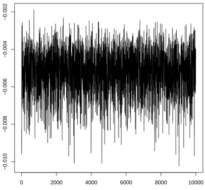
Traceplot The traceplot is a graph of the simulated values against time. When convergence

has been reached, the plot should look like an i.i.d. plot, i.e. the observations should not seem correlated and they should be taking values in all the regions in the support of the target distribution. When this is the case it is usually said that the chain is mixing well. Figure 3.1 was generated using the Metropolis algorithm with the target density in (3.10). The proposal distribution is normal with mean equal to the current state of the chain and variance 0.00001. An example of a chain that does not mix well is given in Figure 3.2. It

0 2000 4000 6000 8000 10000 −0.010 −0.008 −0.006 −0.004 −0.002 Traceplot

Figure 3.1: Good mixing example

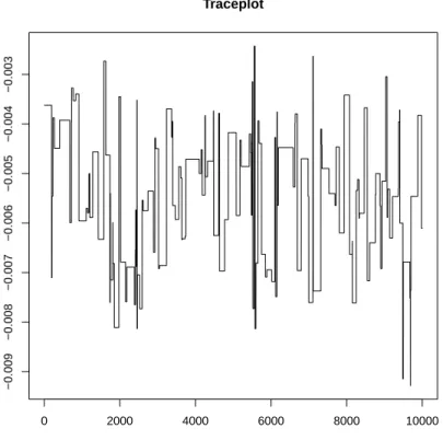
was generated with a chain similar to the one used for Figure 3.1, with the only difference that a variance of 0.01 (instead of 0.00001) was used for the proposal distribution.

(34)

0 2000 4000 6000 8000 10000 −0.009 −0.008 −0.007 −0.006 −0.005 −0.004 −0.003 Traceplot

Figure 3.2: Bad mixing example

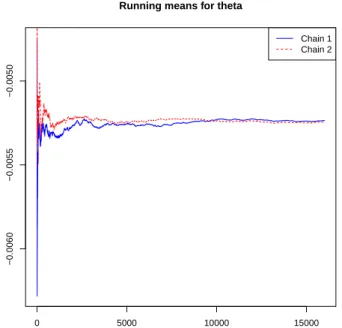
Running Means The running mean at time n is the mean of the first n values of the

simulated chain. A graph of the running mean against time shows whether the mean appears to stabilize as the number of simulations increase. When this is the case, it is evidence that a convergence of type (3.5) is being reached. For this graph it is useful to run parallel chains (this is, to simulate independent chains with the same transition kernel) and plot their running means together to see if they all stabilize at the same value. Figure 3.3 shows the running graph of two parallel chains. They were simulated using stan.

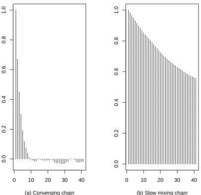
Autocorrelation Plots The k-th lag autocorrelation is defined as

ρk = ∑n−k i=1(Xi−X)(X¯ i+k−X)¯ ∑n i=1(Xi−X)¯ 2 .

It gives the correlation between every simulated value Xi and its k-th lag Xi+k. For a

converging chain, we expect to see ρk get closer to zero as k increases. When this is not the

case, it is a signal of bad mixing. Figure 3.4 shows an autocorrelation plot example for a converging chain and for a bad mixing one.

(35)

0 5000 10000 15000

−0.0060

−0.0055

−0.0050

Running means for theta

Chain 1 Chain 2

Figure 3.3: Running means of two parallel chains

3.3 Monte Carlo Methods and Pseudo Random

Num-bers

To introduce the Monte Carlo method we used the SLLN (Theorem 3.1) as a justification. Nevertheless the “random” numbers given by a computer come from deterministic algorithms that depend only on a initial parameter called the seed. These algorithms are called Pseudo

Random Number Generators (PRNGs). A very common methodology for simulating random

numbers from a specific desired distribution is the following:

Simulation Method 1 (SM1)

1. A PRNG is used to simulate a sequence _{xi}ni=1 of independent uniform(0,1)

numbers.

2. A transformationT is applied to each simulated number in the sequence above. T is chosen in such a way that if U _∼uniform(0,1), then T(U) has the desired distribution. In this way we obtain the sequence _{T(xi)}ni=1 and this is our

(36)

0 10 20 30 40 0.0 0.2 0.4 0.6 0.8 1.0

(a) Converging chain

0 10 20 30 40 0.0 0.2 0.4 0.6 0.8 1.0

(b) Slow mixing chain

Figure 3.4: Autocorrelation plots

Example 3.2. Let us assume that we have a PRNG that simulates independent uniform(0,1)

variates and we want to simulate 5 numbers coming from an exponential distribution with

mean 1. It can be seen that the transformation T(u) = ₋log(1₋u) has the characteristic

explained in Step 2 above. Thus, we first generate 5 numbers with the PRNG. In R this can be achieved with the following code:

(u <- runif(5))

[1] 0.4299841 0.1144878 0.8944409 0.2644449 0.7343649

This is our simulated uniform sequence. Now we apply T to each number above:

-log(1-u)

[1] 0.5620910 0.1215890 2.2484845 0.3071298 1.3256318

and this is a simulation from an exponential(1) distribution. Notice that R has its own

(37)

Now, why do MC methods work with numbers generated from these algorithms? It is clear that the SLLN does not apply since the numbers are not truly random (whatever this means). The answer to this question comes from convergence results in dynamical systems. In what follows we outline how this works. Our exposition is based on G´ora and Boyarsky (1997, Chap. 3).

Definition 3.13. Let(Ω,_F, m) be a probability space. A measurable transformationτ : Ω_→

Ω is said to preserve m if m(τ−1(A)) =m(A) for all A_{∈ F}.

Definition 3.14. Let (Ω,_F, m) be a probability space and let τ : Ω _→ Ω preserve m. The

quadruple (Ω,_F, m, τ) is called a dynamical system.

Definition 3.15. A measure preserving transformation τ : (Ω,_F, m)_→ (Ω,_F, m) is called

ergodic if for any A _{∈ F} with τ−1(A) = A, either m(A) = 0 or m(Ac_{) = 0}_.

In dynamical systems the properties of sequences defined with successive applications of some map τ are studied, i.e. sequences of the type

x0, τ(x0),(τ◦τ)(x0), . . . , τ◦n(x0), . . .

where τ◦n _{means the composition of} _τ _{with itself} _n _{times and}_x

0 is some initial value. The

following is a corollary of Birkhoff’s ergodic theorem. It is the main result of our discussion.

Theorem 3.5. Let (Ω,_F, m, τ) be a dynamical system with τ ergodic and let g be map in

L1(m). Then for m₋almost every x0

1 n n ∑ i=1 g(τ◦i(x0))→ ∫ gdm. (3.11)

This theorem gives sufficient conditions for Monte Carlo integration to converge with a sequence of pseudo random numbers. Let us see how this is the case for SM1.

Assume that we want to use the Monte Carlo method to approximate E[h(Y)] for some measurable function h and a random variable Y that follows some distribution D. Assume also that E[_|h(Y)_|] < _∞, so the L1 _{condition is satisfied. According to the MC}

method-ology we generate N simulations _{yn}N−1n=0 from the distribution D and then we compute

∑N−1

(38)

Let us now use SM1 to generate _{yn}N−1n=0. Suppose you have a dynamical system with

the Lebesgue measure on [0,1] as the invariant measure. Let x0 be an initial value for which

(3.11) is true, and letT be such that ifU _∼uniform(0,1), thenT(U)_∼D. Then a simulated sequence ofDis given byT(x0), T(τ(x0)), . . . , T(τ◦(N−1)(x0)). By Theorem 3.5, we have that

1 N N−1 ∑ i=0 (h_◦T)(τ◦i(x0))→ ∫ 1 0 (h_◦T)(x)dx.

By the change of variable y = T(x), we have that ∫₀1(h_◦T)(x)dx = ∫ hdmD = E[h(Y)],

where mD is the probability measure associated with the distribution D. Thus, if we take

yn=T(τ◦n(x0)), for n = 0, . . . , N −1, we get that N−1

∑

n=0

h(yn)/N →E[h(Y)],

(39)

Chapter 4 Exponential Families and GLMs

In practice insurance portfolios are never homogeneous. An important part of modern pricing is to segment portfolios into aproximately homogeneous groups. From a modelling point of view this allows us to use the knowledge of the properties of homogeneous groups. Afairness

argument is also sensible here: each individual should pay according to the risk they represent. This argument is used for in B¨uhlmann (1967) where it is formulated as follows: “... each class of risk with equal observed risk performance should pay its own way”.

Generalized Linear Models (GLMs) are widely used in practice for segmenting hetero-geneous portfolios and estimate the pure premiums of the resulting classes. In this chapter we give an introduction to GLMs where we emphasize the properties needed to develop our credibility estimate in Chapter 8.

4.1 Exponential Dispersion Families

The definitions and results from this section are based on Jørgensen (1997). A reproduc-tive Exponential Dispersion Family (EDF), is a collection of probability distributions with densities of the form

f(y_|θ, λ) =a(y, λ) exp(λ(θy₋κ(θ))), θ _∈Θ, λ_∈Λ, y _{∈ Y}, (4.1) whereθ and Θ are called the canonical parameter and canonical space, respectively,λ and Λ are the index parameter and set, respectively, and the support of f is _{Y ⊂}R. Also, Θ must

(40)

be an interval and Λ _⊂ (0,_∞). κ is a function called the cumulant generator of the family; it is assumed twice continuously differentiable and κ′′ >0.

Throughout this text whenever the terms exponential families or reproductive families

are used, they refer to (4.1).

Many well known continuous and discrete families of distributions, or transformations of these can be written as an exponential family. The following table shows some examples of well known families of distributions and their respective values of θ, λ, Θ, Λ and κ when written in the form (4.1).

Distribution θ λ Θ Λ κ(θ)

Binomial(n, p) ln(_1−pp ) n R N ln(1+exp(θ)₂ ) Poisson(λ) ln(λ) ₋₋ R ₋₋ exp(θ)₋1 Gamma(α, β) 1₋β α (_−∞,1) R ln(_1−θ1 )

GLMs allow to fit regression models with a response from an exponential family. Some properties of reproductive EDF’s are presented in what follows. We focus on those properties that are essential for the development of GLMs.

The first property concerns the likelihood equation. Assume that we have a random sample from (4.1). Writing the likelihood equation, one can see that the mle for θ does not depend on λ. This property is exploited in estimation procedures for GLMs.

LetY be a random variable whose density can be written as in (4.1). A neat property of the reproductive families is that for θ _∈intΘ (here int stands for interior),

E[Y] = ˙κ(θ) and V[Y] = ¨κ(θ)

λ , (4.2)

where ˙κ = κ′ and ¨κ = ˙κ′ = κ′′. From these two properties we see that the mean and variance are strongly related through κ. The variance function of the family highlights this dependence.

Definition 4.1. Given a reproductive exponential dispersion family, the mean domain of the

family is defined as

(41)

which consists of all the means of the family for which (4.2) holds.

Definition 4.2. The unit variance function of an exponential family is the function V: Ω_→

(0,_∞), with

V(µ) = (¨κ_◦κ˙−1)(µ).

Remark 4.1. We use the symbol V for the variance of a random variable while V is used

for the variance function of an exponential family.

Two important properties of the unit variance function are:

1. V[X] = V(µ)

λ . The name unit variance comes from the fact that V[X] = V(µ) for λ= 1.

2. The unit variance function characterizes the family, i.e. two different exponential dis-persion families cannot have the same unit variance function.

Now consider ˙κ and Θ. The function ˙κ is always continuous and one-to-one. By the continuity of ˙κ, as Θ is an interval, then so is Ω. Sinceµ= ˙κ(θ) and ˙κis invertible, when Θ is an open interval, we can reparametrize the family in terms of (µ, λ)_∈Ω_×Λ. This is called the mean value parametrization of the family. When Θ is not open, i.e. the interval contains at least one of its endpoints, the mean value parametrization can be extended by continuity to the endpoints. Thus, in this way, it is always possible to reparametrize an exponential family with the mean value parametrization.

The support of an EDF depends only on the value of λ. For a given family, let Cλ be the

convex support of any member of the family with index parameter λ. We define the convex support of the family as

C= ⋃

λ∈Λ

Cλ.

Definition 4.3. The unit deviance function of an exponential dispersion family, is defined

as d:C_×Ω_→[0,_∞) with d(y, µ) = 2 [ sup θ∈Θ{ θy₋κ(θ)_{} −}yκ˙−1(µ) +κ( ˙κ−1(µ)) ] . (4.3)

(42)

The unit deviance function plays a very important role in the theory of GLMs. In fact, the model assessment of a GLM is through hypothesis tests that are based on the asymptotic behavior of this unit deviance function. Some of its important properties are:

1. The unit deviance and variance functions are related by the equation ∂2

∂µ2d(µ, µ) =

2

V(µ).

2. The unit deviance function characterizes the family.

3. The mean value parametrization of a reproductive exponential dispersion family can be written as

p(y;µ, λ) =c(y, λ) exp

(

−λ

2d(y, µ)

)

, (4.4)

for some function c.

Regular exponential families are an important particular case of exponential families.

Definition 4.4. A reproductive exponential dispersion model is called regular if its canonical

space Θ is open.

Regular families have some important properties that will be used later:

1. For any given family, we have Ω_⊂Cλ, and hence Ω⊂C. For regular families we have

Ω =C.

2. Wheny, µ_∈Ω, the unit deviance function can be written as

d(y, µ) = 2[y_{κ˙−1(y)₋κ˙−1(µ)_{} −}κ( ˙κ−1(y)) +κ( ˙κ−1(µ))], (4.5) which is easier to work with than the original definition since the sup in (4.3) disappears so (4.5) can be used as the definition of the unit deviance for regular families.

3. For y, µ_∈Ω, the deviance can be written as d(y, µ) = 2

∫ y

µ

(y₋t)

V(t) dt. (4.6)

(43)

4.1.1 Weights and Data Aggregation

There is a decomposition of the index parameter in (4.1) that has been appropriate in several contexts; one of them being GLMs. It consists in takingλ = w_ϕ. wis known as the weight and ϕ as the dispersion parameter. The weight is assumed to be known and it is not considered a new parameter of the distribution. Thus, allowing ourselves the little abuse of notation of using the same function name a, (4.1) becomes

f(y_|θ, ϕ) =a(y, ϕ) exp ( w ϕ{yθ−κ(θ)} ) . (4.7)

There is a useful property of reproductive exponential dispersion families parametrized as above that allows for data aggregation. Jørgensen’s notation (from Jørgensen (1997)) is very convenient for expressing this property: given a fixed exponential family, ifY has mean µand density given by (4.7), we say that it isED(µ, ϕ/w) distributed. The property is then as follows: if Y1, Y2,· · · , Yn are independent, and Yi ∼ED(µ, ϕ/wi), then

¯ Y = w1Y1+· · ·+wnYn w+ ∼ ED(µ, ϕ/w+), w+= n ∑ i=1 wi. (4.8)

4.1.2 A Note on Aggregating Discrete Exponential Dispersion

Mod-els

There are two usual parametrizations of exponential dispersion families. (4.1) gives the den-sity of reproductive EDFs and it is used for continuous distributions. Discrete distributions are usually parametrized as additive EDFs, whose densities have the form

f(y_|θ, ϕ) =a(y, ϕ) exp (yθ₋λκ(θ)), θ _∈Θ, λ_∈Λ. (4.9) Both parametrizations are defined and discussed in Jørgensen (1997) and Jørgensen (1992). An aggregation property different than (4.8) holds for additive EDFs. In Jørgensen’s no-tation, given a fixed additive EDF with density (4.9) and mean µ, we say that it follows a ED∗(µ, λ). If Y1, . . . , Yn are independent and Yi ∼ED∗(µ, λi), then

Y1+· · ·+Yn∼ED∗(µ, λ+), λ+=λ1+· · ·+λn.

As shown in the next section, GLMs assume the reproductive parametrization (see also Nelder and Wedderburn (1972)). Now, for many discrete EDFs, the dispersion parameter has

(44)

a known value. Specifically, for the Poisson, Bernoulli and negative binomial distributions Λ =_{1_}. This makes (4.1) and (4.9) the same parametrization and allows such distributions to enter the GLMs framework. Nevertheless, it is important to be aware that for GLMs with a discrete response distribution, one cannot aggregate data using (4.8). The properties of the Poisson distribution allow to use an offset for this purpose (see for example Kaas et al. (2008)) and quasi-likelihood can be used for other discrete distributions.

4.2 GLMs

In a GLM the response variable is assumed to follow a reproductive exponential dispersion family with density (4.7). Notice that since (4.7) is equivalent to (4.1) with λ= w_ϕ, then the mean and variance of the response variable can be expressed asµ=κ′(θ) andσ2 ₌_ϕκ′′_(θ)/w,

respectively. It is further assumed that there is a vector of explanatory variables, also known as covariates, x= (x1,· · · , xp), a vector of coefficients β = (β0, β1,· · · , βp) and a function g

such that

g(µ) =β0+x1β1+· · ·+xpβp. (4.10)

It is useful for further developments to express the canonical parameter θ in terms of the coefficients. Since µ= ˙κ(θ) then:

(g_◦κ)(θ) =˙ β0+x1β1+· · ·+xpβp

θ = (g_◦κ)˙ −1(β0+x1β1+· · ·+xpβp). (4.11)

Notice that the population can be divided into different classes according to the values of the explanatory variables. Thus, given a sample, we can group together all the observations that share the same values of explanatory variables and aggregate them with (4.8). It is important to mention that with this grouping there is no loss of information for estimating the mean since ¯Y is a sufficient statistic for θ ( but not for ϕ, thus some information is lost for the estimation of ϕ).

After aggregating, let m be the number of classes and θ = (θ1,· · · , θm) a vector whose

(45)

others and therefore the density of the sample can be expressed as f(y_|θ, ϕ) =a(y, ϕ) exp ( yT_W_θ₋₁T_W_κ₍_θ₎ ϕ ) , y_∈Rm_, _(4.12)

where κ(θ) = (κ(θ1),· · ·, κ(θm)), W = diag(w1,· · · , wm), wi is the sum of all the weights in

the i-th class, 1= (1,_{· · ·} ,1) and a(y, ϕ) =∏m

i=1(a(yi, wi

ϕ)) . In order to express θ in terms

of β, we define the following maps

µ=κ˙(θ) = ⎛ ⎜ ⎜ ⎜ ⎝ ˙ κ(θ1) .. . ˙ κ(θm) ⎞ ⎟ ⎟ ⎟ ⎠ , G(µ) =G ⎛ ⎜ ⎜ ⎜ ⎝ µ1 .. . µm ⎞ ⎟ ⎟ ⎟ ⎠ = ⎛ ⎜ ⎜ ⎜ ⎝ g(µ1) .. . g(µm) ⎞ ⎟ ⎟ ⎟ ⎠ ,

and the design matrix

X = ⎛ ⎜ ⎜ ⎜ ⎝ 1 xT 1 .. . 1 xT m ⎞ ⎟ ⎟ ⎟ ⎠ ,

where xi is the vector of explanatory variables for the i-th class. With all this definitions,

we have that

G(µ) =Xβ, (G_◦κ˙)(θ) =Xβ,

θ= (G_◦κ˙)−1(Xβ). (4.13) When µand β have the same dimension we say that the model issaturated. In this case one can find a value of β for which the predicted means are equal to the observed means. In practical applications the dimension of β is usually less than the dimension ofµ. This is called a non-saturated model.

It is useful to reparametrize (4.12) in terms of the mean vectorµinstead of θ. Using the mean value parametrization (see (4.4)), (4.12) can be reparametrized as

f(y|µ, ϕ) =c(y, ϕ) exp ( − 1 2ϕD(y,µ) ) , (4.14) where c(y, ϕ) =∏m i=1c(yi, ϕ wi), and D(y,µ) = m ∑ i=1 wid(yi, µi). (4.15)

(46)

• Given a sample, finding the mle of θ is equivalent to finding the value of β that minimizes the deviance.

• Dcan be used to estimate the dispersion parameter (although it is not the only method). The deviance estimator of ϕ is given by

ˆ

ϕ = D(y,µ) n₋p .

• The asymptotic distribution of D plays an important role in model assessment and variable selection.

For further details about the use and properties of the deviance we recommend Jørgensen (1992).

Remark 4.2. GLMs allow categorical and continuous variables. In an insurance context

their different values divide the population into homogeneous groups. Since it is desirable to have numerous observations in each group, it is a common practice to divide continuous variables into intervals so they can be treated as categorical.

(47)

Chapter 5 Relative entropy

In this section, let mi, i = 1,2 be probability measures with dmi(x) = fi(x)ds(x), for some

functionsf1, f2 and some probability measures. It is also assumed thatm1 ≡m2 ≡s, where

m1 ≡m2 means that m1 and m2 are equivalent measures.

Definition 5.1. The relative entropy of m2 from m1 is defined as

D(m1||m2) = Em1 [ log ( f1(X) f2(X) )] = ∫ log ( f1(x) f2(x) ) dm1(x). (5.1)

The definition above was introduced by Kullback and Leibler (1951). D(_·||·) is often called the Kullback-Leibler divergence, although what they called divergence is the sum D(m1||m2) +

D(m2||m1) (I(1 : 2) +I(2 : 1) in their own notation). Therefore we have decided to use

another common name used for (5.1): relative entropy.

We give now a statistical interpretation of this definition. It is taken from Kullback (1968), Chapter 1. Assume we have two hypothesesH1andH2 about the distribution ofX;Hi is the

hypothesis that X is distributed according to mi, i = 1,2. Assume also prior probabilities

P(Hi),i= 1,2 for these hypotheses. One can show that the posterior probabilities P(Hi|X)

satisfy

P(Hi|X) =

P(Hi)fi(X)

P(H1)f1(X) + P(H2)f2(X)

[s], i= 1,2. From this relation, we can obtain

log ( f1(X) f2(X) ) = log ( P(H1|X) P(H2|X) ) −log ( P(H1) P(H2) ) . (5.2)

(48)

Now, P(H1) P(H2) and

P(H1|X)

P(H2|X) are the prior and posterior odds ofH1, respectively. Hence, the right

hand side in (5.2), is the difference between the logarithm of the odds of H1 after and before

observing the value of X. Thus, given X = x, the likelihood ratio log(f1(x) f2(x)

)

is defined as the information for discriminating in favour of H1 againstH2. D(m1||m2) is the integral with

respect to m1 of the left hand side in (5.2). Therefore, D(m1||m2) is the mean information

in favor of H1 against H2 per observation from m1.

5.1 Properties

Additivity

The relative entropy of a vector of independent random variables is equal to the sum of the relative entropies of the marginal distributions. In other words, if Hi states that for

measurable sets A and B, mi(A×B) = mix(A)miy(B) for i= 1,2, then

D(m1||m2) = D(m1x||m2x) +D(m1y||m2y).

Convexity

Theorem 5.1. D(m1||m2)≥0 with equality if and only if m1 =m2.

Invariance

Let (Ω1,F, mi) and (Ω2,G, νi), for i = 1,2, be probability spaces and T : Ω1 → Ω2 a

measurable transformation such that νi(G) = mi(T−1(G)), for G ∈ G. Define also γ(G) =

s(T−1(G)). Since m1 ≡ m2 ≡ s, then ν1 ≡ ν2 ≡ γ. This implies, by Radon-Nykodim’s

theorem that there exist g1 and g2 such that

νi(G) =

∫

G

gi(y)dγ(y), G∈ G.

With these definitions in mind, the following theorem asserts the invariance property of the relative entropy. Its proof can be found in Chapter 2 of Kullback (1968).

(49)

Lower Bound: The Total Variation Distance

The relative entropy is not a metric since it is not symmetric and it does not satisfy the triangle inequality. Nevertheless it is usually interpreted as a measure of how different two probability measures are. It also provides a bound on the total variation between two prob-ability measures.

Theorem 5.3. Let dT V(P, Q) = supB∈F|P(B)−Q(B)| be the total variation distance in

some measurable space (Ω,_F), for two probability measures P and Q. Then

D(P_||Q)_≥ dT V(P, Q)

2

2 .

A proof of this result can be found in Kemperman (1969).

5.2 Relative Entropy and Maximum Likelihood

Esti-mation

Consider the case when a parametric model is assumed in some given situation. Let Θ be the parameter space and νθ the model’s probability measure for a given parameter θ ∈ Θ.

In this section we give a proof that, asymptotically, a maximum likelihood estimator (mle) minimizes the entropy between the true distribution and the assumed model. This property was introduced in Akaike (1973), but the result is only commented in the paper with no formal proof nor specifying sufficient conditions. We give in this section a set of assumptions under which the result is true and prove it.

Let m be the true probability measure, the first assumption is:

(A1) For every θ _∈ Θ, m and νθ are absolutely continuous with respect to some common

probability measure s.

Due to this assumption there exists a measurable function f such that dm(x) = f(x)ds(x), and for every θ _∈ Θ there exists fθ such that dνθ(x) = fθ(x)ds(x). This takes us to our

second assumption:

(50)

Given thatX1,· · · , Xn are iid andm-distributed, the log-likelihood function for our assumed model is defined as ℓn(θ) = n ∑ i=1 log(fθ(Xi)).

Notice that by Assumption 2 and the strong law of large numbers, we have that ℓn(θ)

n −→Em[log(fθ(X1))] [m]. (5.3) For every N _∈N, defineDN _as

DN(m_||νθ) = Em[log(f(X1))]−

ℓN(θ)

N , and note that by (5.3) we have for every θ_∈Θ, that

DN(m_||νθ)−→D(m||νθ) [m]. (5.4)

Let ˆθn be a maximum likelihood estimator of θ. In other words,

ˆ

θn = argmax θ ℓn(θ),

which also means then that ˆθN minimizes DN(m||νθ) over the set θ ∈Θ. We state now the

third assumption:

(A3) There exists an mle for θ for every n _∈N.

The fourth and final assumption simply states that it is possible to minimize the entropy between the true distribution and the assumed model:

(A4) There exists θ0 ∈Θ such that for every θ ∈Θ,D(m||νθ0)≤D(m||νθ).

Remark 5.1. It is not being assumed that m belongs to the hypothesized model; i.e. we do

not suppose that there exists θ∗ _∈Θ such that f =fθ∗.

Notation 5.1. To simplify notation in the following proofs, DN_(θ) _and _D(θ) _{are used for}

Computational Bayesian Methods for Insurance Premium Estimation