Master in Artificial Intelligence
Using peptidomics and machine learning techniques
to predict mortality of patients with septic shock
In collaboration with the ShockOmics study
Submitted by Helen Byrne
April 2018 Supervisor: Alfredo Vellido
Department of Computer Science, Universitat Politècnica de Catalunya Co-supervisor:
Vicent Ribas Ripoll ShockOmics, Eurecat
Contents
1 Introduction 2 2 Background 4 2.1 Shock . . . 4 2.2 Sepsis . . . 5 2.2.1 Septic Shock . . . 62.3 State of the art . . . 7
2.3.1 Proteomics . . . 7 2.3.2 Peptidomics . . . 7 2.3.3 Patient prognosis . . . 8 2.4 Machine learning . . . 9 3 Methods 11 3.1 Data . . . 11 3.1.1 Data preprocessing . . . 14 3.2 Data Analysis . . . 16 4 Experiments 18 4.1 Experimental settings . . . 18 4.1.1 Feature Importance . . . 18 4.1.2 Classification . . . 20 4.2 Experimental Results . . . 23 4.2.1 Feature Importance . . . 23
4.2.2 Classification using Important Features . . . 25
5 Conclusions 35 References 37 A Appendix 42 A.1 Important features . . . 42
List of Figures
3.1 Outcome of patients (NS=NonSurvivor, S=Survivor) . . . 12 3.2 Pictorial representation of septic shock patient peptidome data after
initial data preprocessing steps . . . 14 3.3 Sample distributions of 3 T1 peptides chosen at random; (l-r) peptides
831, 238, 241 . . . 16 3.4 Boxplots showing distribution of T1 (log2 transformed) peptides with
biggest differences in mean abundance between survivors and non-survivors . . . 16 3.5 Boxplots showing distribution of T2 (log2 transformed) peptides with
biggest differences in mean abundance between survivors and non-survivors . . . 17 4.1 T2 SVM coefficients . . . 28 4.2 Distribution for NS and S of peptides used to classify patient outcome.
Top row (l-r): Peptides important to classify NS from most to least; bottom row (l-r): Peptides important to classify S from most to least. 31 4.3 Plot of abundances of peptides used in 100% accuracy classification
result: (l) Top 3 peptides used for classification by SVM; (r) Top 3 NS features used for classification by SVM . . . 32 4.4 Heatmap of abundances of peptides used in 100% accuracy
classifi-cation result [Key: S samples are top 23; NS samples are bottom 6] . . . 32 4.5 T2 SVM coefficients from 99% accuracy model . . . 33 4.6 Plot of abundances of peptides used in 99% accuracy classification
result: (l) Top 3 peptides used for classification by SVM; (r) Top 2 features used for classification by SVM . . . 33
List of Tables
3.1 Patient demographics & SOFA, APACHE II scores Format: Mean(±
s.d.) . . . 13 4.1 Baseline metrics results . . . 26 4.2 T1 mean 5-fold CV classification results, using features selected by
RF algorithm (best 50 features: rf50) and XGBoost algorithm (xgb) . 27 4.3 T1 LOOCV classification results, using features selected by RF
algo-rithm (best 50 features: rf50) and XGBoost algoalgo-rithm (xgb) . . . 28 4.4 T2 mean 5-fold CV classification results, using features selected by
RF algorithm (best 50 features: rf50) and XGBoost algorithm (xgb) . 29 4.5 T2 LOOCV classification results, using features selected by RF
algo-rithm (best 50 features: rf50) and XGBoost algoalgo-rithm (xgb) . . . 30 4.6 T2 classification results using features selected by XGBoost algorithm
(xgb) . . . 31 4.7 T1_T2 mean 5-fold CV classification results, using features selected
by RF algorithm (best 50 features: rf50) and XGBoost algorithm (xgb) 33 4.8 T1_T2 LOOCV classification results, using features selected by the
RF algorithm (best 50 features: rf50) and XGBoost algorithm (xgb) . 34 A.1 50 most important features selected by random forest algorithm on
original (not SMOTE) T1 data . . . 43 A.2 50 most important features selected by random forest algorithm on
T1 SMOTE data . . . 44 A.3 Most important features selected by XGBoost algorithm on original
(not SMOTE) T1 data . . . 44 A.4 Most important features selected by XGBoost algorithm on SMOTE
T1 data . . . 44 A.5 50 most important features selected by random forest algorithm on
original (not SMOTE) T2 data . . . 46 A.6 50 most important features selected by random forest algorithm on
SMOTE T2 data . . . 47 A.7 Most important features selected by XGBoost algorithm on original
(not SMOTE) T2 data . . . 47 A.8 Most important features selected by XGBoost algorithm on SMOTE
T2 data . . . 47 A.9 50 most important features selected by random forest algorithm on
A.10 50 most important features selected by random forest algorithm on
SMOTE T1T2 data . . . 49
A.11 Most important features selected by XGBoost algorithm on original (not SMOTE) T1T2 data . . . 50
A.12 Most important features selected by XGBoost algorithm on SMOTE T1T2 data . . . 50
A.13 T1 classifier parameters . . . 50
A.14 T2 classifier parameters . . . 51
Abstract
The main objective of this thesis is to analyse peptidomics data and evaluate their use in the prediction of risk of death of patients in septic shock. The World Health Organisation reports [1] that there are up to 24 million cases of septic shock globally, each year, and incidence is rising. Further, it has mortality rates of 40%, but yet is still little understood. The early detection and treatment of sepsis and septic shock represent big medical challenges and as yet there are no known biomark-ers for its prediction. This thesis hopes to determine if there exists any correlation between patient peptidome and their mortality. The plasma peptide levels data used in this thesis was collected by mass spectrometry-based peptidomics as part of the ShockOmics European research project, the first of its kind to try and eval-uate causes of shock. This is the first time this peptidome data has been analysed in this depth. Machine learning techniques were implemented for feature selection and classification. The resulting classification of patient outcome, from patient pep-tidome taken 48 hours after shock diagnosis, was largely successful, with one model obtaining 100% mean accuracy. Using this model, we were able to identify 8 relevant peptides that may provide some clinical insight into the pathophysiology of septic shock. These results are discussed and suggestions made for future research.
1
|
Introduction
Sepsis is a major public health concern, making up about 21% of all patients admit-ted to ICU [2] and one of the main causes of death for patients in ICU. Furthermore, the number of cases are steadily rising due to ageing populations and increases in comorbidities e.g. diabetes, cancer. This trend is set to continue in the foreseeable future.
Sepsis is described as life-threatening organ dysfunction caused by the body injuring its own tissues and organs in response to infection [3]. It is the number one cause of death from infection, with mortality rates of 10%. The most severe cases of sepsis lead to septic shock, which entails mortality rates of over 40%. The heterogeneity with which symptoms are exhibited by septic patients make it difficult to diagnose. According to the latest definitions [3] it can be clinically identified by an increase in SOFA (Sequential [Sepsis-related] Organ Failure Assessment) score of 2 or more, but this cannot be ascertained at bedside and therefore a quick (bedside) SOFA score has also been developed.
Although sepsis and septic shock cases comprise such a large proportion of ICU admissions, there is still no simple, unambiguous criterion to uniquely identify a patient with sepsis [3]. Further, little progress has been made in improving mortality rates and outcome is still difficult to predict [4]. Whilst the SOFA scores are able to give guidance on patient outcome a definitive prediction, diagnosis and personalised treatment is needed to improve patient outcome. The top management technique for patients in septic shock is “early recognition”. Therefore, rather than a reactive treatment to attempt to reduce shock symptoms, it is important to be able to identify the causes, biomarkers and indications of developing shock.
Due to rapid technological advancements and high-throughput techniques, we are now able to analyse large amounts of high-dimensional data, like omics data. Omics data has huge potential and applications. It has the ability to explain normal physi-ological processes, to describe the aetiology of diseases and identify disease biomark-ers. In this thesis, machine learning techniques will be applied to peptidomics data from patients with septic shock, to attempt to identify patterns within it and learn and rank important features of the data that can be included in a model predicting patient outcome. In doing this, we aim to deduce what are the most important features of patient peptidomics data, relative to their risk of death, and use this information to guide patient therapies. Further, this acquired knowledge can inform future research into the aetiology and early, unambiguous diagnosis of septic shock. The next chapter, Chapter 2: Background, of this thesis provides vital
back-ground information into the understanding of the machine learning task. Firstly with scientific knowledge on shock, sepsis and septic shock; followed by a summary of the state of the art of the research into these, specifically using proteomics, pep-tidomics and machine learning techniques. Chapter 3: Methods continues with a
detailed description of the data used in this project; its collection, preprocessing, and analysis. Chapter 4: Experiments gives a comprehensive account of the
experi-ments undertaken in this study, it summarises the experimental settings, significant results accompanied by a discussion of these results for feature selection of peptides and classification of patient outcome. Finally,Chapter 5: Conclusions discusses the
highlights and meaning of the results of this project and what further study they lead on to.
2
|
Background
2.1
Shock
Shock is a serious condition in which there is insufficient blood flow throughout the body, which deprives the organs and tissues of oxygen. Initially, shock is reversible, but if it is not recognised and treated immediately, it can progress to irreversible organ dysfunction. [5] There are four main subtypes of shock, all of which result in hypoperfusion to organs, but have different causes: cardiogenic, hypovolemic, ob-structive and distributive. These subtypes of shock are not exclusive, and patients can experience a combination of more than one type of shock.
Cardiogenic shock is caused by heart damage. The heart is no longer able to pump sufficient blood around the body. The most common cause is from a severe heart attack. [5]
Hypovolemic shock is caused by severe blood or fluid loss, which means the heart can no longer pump enough blood around the body. Or severe anaemia, in which the blood cannot carry enough oxygen around the body. [5]
Obstructive shock is caused by an obstruction in the bloodflow outside of the heart. There are several conditions that can result in obstructive shock, in-cluding aortic dissection: in which the aorta tears and can no longer transport blood to and from the heart, and vena cava syndrome: in which the vena cava vein is blocked and can no longer carry blood back to the heart. [5]
Distributive shock is caused by blood vessels dilating too much, so that they are unable to continue circulating blood sufficiently around the body. The most common cause is from sepsis, caused by an overwhelming infection, which leads to septic shock. Another cause is a severe allergic reaction, leading to anaphylactic shock. Distributive shock can be viewed as different from the other 3 types because it is the only kind that occurs even though the heart is still working at a normal output level. [5]
The most common type overall is hypovolemic shock [6]. However, septic shock is the most common form of shock seen in patients admitted to ICUs, and the biggest cause of death of patients in ICUs. Whilst hypovolemic and anaphylactic shock can usually be readily treated, septic shock is a much greater concern with mortality rates of over 40%. Cardiogenic shock has the worst patient outcome and is associated with 70%-80% in-hospital mortality [7].
heartbeat. Other symptoms show in varying degrees and depend on the cause and severity. Additionally, the best treatment is dependent on the cause and severity of shock. Usually, the treatment is to identify and negate the cause of shock as quickly as possible.
Shock is a physiologic continuum [5], which begins with an event, e.g. an infection. It progresses through pre-shock and shock, which are reversible, treatable stages. The final and irreversible stage, end-stage shock, leads to multiple organ failure and death. It is clearly of utmost importance that the cause of shock is identified as quickly as possible, so that it can be treated before a patient reaches end-stage shock. Better still, a means of early identification and preventative treatment is needed, particularly for shock types with high mortality rates, like septic and cardiogenic shock.
2.2
Sepsis
Sepsis is the body’s overwhelming response to infection. In most cases of infection the body is able to respond adequately to target the infection and, in the case of bacterial infections, a course of antibiotics can even more efficiently kill the infection. However, in some severe cases, the body attempts to fight the infection, but causes extensive inflammation, blood clots and leaking blood vessels [8]. The body can no longer receive sufficient blood, and the organs and tissues are deprived of oxygen.
Sepsis has been defined in the latest definitions [3] as “life-threatening organ dysfunction caused by a dysregulated host response to infection”. It is the condition that costs the most for U.S. hospitals each year, costing $24 billion in 2013 [9] and one report estimates that it affects 18 million people worldwide, each year, of which 5 million die [10]. Furthermore, the incidence of sepsis has increased 13.7% in the past 30 years. This is probably because of an ageing population, with more comorbidities, but could also reflect a push for better understanding and diagnosis of sepsis.
The source of sepsis can be many different types of microbes, and often it is difficult for doctors to identify the original source of infection. Common sources of infection are in the lungs e.g. pneumonuia; urinary tract; and abdomen e.g. peritonitis. Sepsis mostly affects old and very young people, but also those with a weakened immune system, maybe due to another condition such as AIDS or cancer. Sepsis can be clinically characterised using the SOFA score, which evaluates organ dysfunction. “Organ dysfunction can be identified as an acute change in total SOFA score ≥ 2 points consequent to the infection [3].” This increase in score
correlates with an overall mortality risk of approximately 10%.
Some components of the SOFA score cannot be immediately measured, but re-quire laboratory testing. Therefore, the Quick SOFA (qSOFA) criterion is defined additionally, to be used as a prompt bedside diagnostic, which can be followed-up with full SOFA scoring by laboratory testing. qSOFA criteria [3] is identified as:
Respiratory rate ≥22/min
Altered mentation
One of the biggest challenges of sepsis is the heterogeneity with which it affects patients. Different patients with sepsis have different aetiology, susceptibility, re-sponses and require different treatment [11]. This means that patients often exhibit symptoms at different times and with different levels of severity, and therefore they are not diagnosed in the earliest stage of sepsis, which is directly linked to an in-creased mortality risk. Given that sepsis occurs so frequently and with such poor prognosis, it is vital to identify improved prediction of patient prognosis and person-alised treatment. At the moment it transpires quite unpredictably and progresses quickly. An improvement in prevention, prediction and treatment would lead to a huge improvement in overall hospital mortality rates.
2.2.1
Septic Shock
The most severe cases of sepsis develop into septic shock, with increased mortality rates of 40%. Septic shock is described in the latest definitions in [3] as “a subset of sepsis in which particularly profound circulatory, cellular, and metabolic abnormal-ities are associated with a greater risk of mortality than with sepsis alone.” It can be clinically diagnosed by:
(i) A vasopressor requirement to maintain a mean arterial pressure (MAP) of ≥65
mm Hg, and
(ii) Serum lactate level > 2 mmol/L (>18 mg/dL) in the absence of hypovolemia (a decrease in blood volume). [3]
This means that a patient in septic shock experiences hypotension (low blood pressure) and vasopressor therapy is needed in order to maintain this pressure at sufficient levels (i.e. MAP ≥ 65 mm Hg). Additionally, septic shock patients have
elevated lactate levels in their blood.
This newly-defined clinical diagnosis of septic shock requires a blood sample to be analysed in order to measure for elevated lactate levels. The definitions’ taskforce [3] acknowledged that these measurements are not universally available, especially in developing countries. Furthermore, even where lactate measurements are possi-ble, diagnosis is not possible in real-time in ICU, due to the time taken to obtain these measurements. It is known that doctors must act quickly to treat patients in septic shock, and so there is not enough time to obtain these measurements and to diagnose the patients according to these definitions. In fact, most patients are clinically diagnosed later, after treatment for septic shock has started. Furthermore, although elevated lactate levels are certainly reflective of cellular dysfunction in sep-sis, leading to septic shock, there are many other factors that similarly contribute to and result in these increased levels. Increased blood lactate levels reflect a "com-plex metabolic disturbance", but not necessarily as a direct result of sepsis/septic shock [12]. Sepsis and septic shock, therefore, are often a challenge for doctors to diagnose. Their clinical symptoms are also symptoms for other disorders, which are seen in higher percentages of patients, and so they are misdiagnosed. [13] lists 84 disorders that have similar symptoms and are often diagnosed instead of sepsis. Due to this challenge and the rapid rate at which septic shock develops to a fatal outcome, diagnosis can often occur too late to save the patient.
It would clearly be a major breakthrough, and improvement for patients in both developed and developing countries, if another means of identifying the onset of
septic shock is identified, which can either be measured in real-time or used for prediction of septic shock. This thesis hopes to help in this line of research, by identifying predictors of septic shock patient outcome from peptidome analysis.
2.3
State of the art
Encouragingly, there appears to be much ongoing research into discovering solutions to the problems already discussed and more. The US National Institute of Health (NIH) keeps track in its onlineRePORT [14] of ongoing and published NIH-funded
projects and clinical trials. In this database, 180 active projects are found with titles including “sepsis” or “septic shock”. These projects include research into pathology, treatment, body response and recovery from sepsis and septic shock. Others include research with specific populations, for instance “pediatric sepsis”, “neonatal sepsis” and “sepsis in the elderly”.
2.3.1
Proteomics
In recent years, with the massive improvements in computational power and genetic understanding, there has been a big increase in research using omics techniques, such as proteomics. Proteomics refers to the study of proteomes and also the tech-niques used to identify the proteome of an organism, like mass spectrometry (MS). MS enables the analysis of proteomes; first the proteome is separated, then the proteins are characterized by MS by comparing the masses of the proteins or pep-tides to calculated masses from genome data [15]. MS-based proteomics has been a powerful tool, driving invaluable insights into sepsis. A 2014 review [16] into “pro-teomics studies of sepsis” details some of the most important studies from recent years. These include the discovery of many biomarker candidates of septic infection, which could remarkably improve diagnosis and treatment of sepsis and septic shock. Paiva’s study [17] from 2010, used proteome techniques to analyse serum protein expressions at each stage of sepsis. From these, 14 differentially expressed proteins were identified, as well as a potential biomarker. Furthermore, the study concluded the involvement of genetic information in sepsis.
More recently, in [18], using proteomics, a parasite-protein is found to be able to combat disorders that cause mitochondrial dysfunction, such as sepsis. Additionally, [19] uses quantitative targeted proteomics to investigate the processes that manage
the composition of plasma proteome, in doing so, changes of plasma proteome from mouse animal models with sepsis are determined. In general, the results of pro-teomics are a list of proteins or further, the ways in which these proteins are seen to be interacting. This knowledge can lead to better understanding of molecular pro-cesses during sepsis, leading to development of targeted treatments. It is clearly an area of sepsis research likely to continue growing and developing, hopefully leading to important discoveries in the near future.
2.3.2
Peptidomics
One subdiscipline of proteomics is peptidomics. Peptidomics is the comprehensive qualitative and quantitative analysis of all endogenous (originating within the
organ-ism) peptides in a biological sample. The term first appeared in a paper in 2001 [20], and is now included in over 1200 publications. Endogenous peptides have a wide range of functions; as hormones, neurotransmitters and antimicrobial agents [21]. These important and diverse roles played by peptides mean that they offer great potential for medicine research. Targeting peptide hormone pathways has been a successful strategy in the development of novel therapeutics [21].
Peptidome analysis is a challenging technique (more so than proteome analysis), due to several factors. These include protease digestion during sample preparation, computational challenges in data analysis, and relying on a single identification be-cause each peptide is present in the peptidome only once [22]. Despite this, research utilising peptidomics has proved its worth, spanning the design of immunotherapies for the treatment of hematologic (blood) cancer [23] and identification and predic-tion of HLA (Human leukocyte antigen)-associated peptides [24], offering potential for design of more effective vaccines for infections and cancer.
As a fairly recent area of study, it will undoubtedly contribute to a lot more in the future, including studies in and related to sepsis and septic shock. As yet, little research has been done utilising the power of peptidomics in sepsis research. To the best of our knowledge, just a few studies exist so far. This could be because, until now, not enough peptidome data of septic patients had been collected to warrant its use in research. The state of the art in this domain is comprised of a couple of studies into proteolytic activity during shock. In [25], the peptidome of healthy and hemorrhagic shock (HS) rats was compared and an increase in peptides after hem-orrhagic shock was found, confirming proteolytic activity is part of the pathologic phenomena occurring in hemorrhagic shock. Additionally, in [26], this hypothesis is tested using patient data for the first time and the results suggest that autodiges-tion is a fundamental mechanism for organ dysfuncautodiges-tion and outcome in septic shock. Presently, these are the only studies that we are aware of, investigating peptidomics and sepsis/shock.
2.3.3
Patient prognosis
Patient prognosis is important as it plays a central role in medical decision-making, guiding patient treatment. Prognosis helps doctors move from general diagnosis to personalised treatment for a given patient. Unfortunately, regarding sepsis and septic shock, prognosis is little understood and the molecular mechanisms that lead from sepsis to septic shock to patient outcome have not yet been determined. The current best prognostic tools used by doctors are generic clinical severity scores such as Acute Physiology and Chronic Health Evaluation (APACHE)II. This score is used for all critically ill patients, to give a general idea of their illness severity, and includes no specificity for sepsis. Therefore, unsurprisingly, it is a suboptimal prognostic tool for septic patients and something more specific to the disorder needs to be identified. Research to this end has been attempted for many years. In 1978, a study [27] analysed the blood plasma of septic patients and identified an increase in total amino acid content, additionally it was found that patients that did not survive had “higher levels of aromatic and sulfur-containing amino acids as compared to those patients surviving sepsis.” The study concluded from these results, an idea for therapy to positively affect patient outcome. In recent years,
there has been a number of studies into patient prognosis. In [28], metabolites are identified that could discriminate between septic shock and control patients, thus serving as potential biomarkers for septic shock. In [29], the prognostic value of presepsin was investigated. It was found to be related to patient outcome but its effectiveness as a biomarker to guide treatment has yet to be demonstrated.
It is hoped that with new omics techniques, we will be able to shine a light on the molecular mechanisms that are occurring through the different stages of sepsis. In [30], an omics approach similar to this project was taken, but with metabolomics. The study identified changes in plasma levels of lipid species and kynurenine showed links to patient mortality, requiring followup investigation to determine potential implications for new targeted therapy. Furthermore, a 30-day mortality prognostic model was designed [31] using transcriptomic data which shows significant improve-ment on clinical severity scores. The next test is to translate these models into usable bedside tests that can provide fast and accurate guidance for medical professionals in the treatment of sepsis.
2.4
Machine learning
The use of machine learning techniques in medical research is a promising combina-tion. With increased computational strength, we are now in a position to perform analytics on huge datasets, that previously were not possible. Machine learning by definition requires vast amounts of data, which lends itself naturally to the (data de-pendent and data generating) critical care department (CCD), where patients with sepsis are treated. These large quantities of collected data are being combined with a broad selection of machine learning methods to solve diverse problems like defining medicine dosing, creating patient-specific alarm algorithms in real-time, assessing patient prognosis in sepsis and predicting mortality of patients [32]. In addition to new data collected specifically for research today, large datasets collected previously can be accessed and utilised. This is, for instance, seen in the Sepsis definitions of [3], in which the electronic health records of 1.3 million encounters from 12 hos-pitals in southwestern Pennsylvania along with 700,000 patients from external US and non-US datasets were studied in order to conclude a means to clinically char-acterize a septic patient. Additionally, the Medical Information Mart for Intensive Care (MIMIC) database is one that has been used by several studies into sepsis, utilising machine learning. It comprises the records of 40,000 critical care patients, and includes demographics, vital signs, laboratory tests and more. An “Artificial Intelligence Sepsis Expert” was developed [33] to assist in the prediction of the on-set of sepsis, using the MIMIC database information of 65 features per hour of vital signs and electronic medical record data. Another predictor of sepsis, the InSight algorithm, is described and evaluated using the MIMIC dataset in [34]. In [35] and [36], it is evaluated with additional data and in a randomised controlled trial and found to lead to reductions in patient mortality and length of stay. The identifica-tion of biomarkers of disease is another important area of research, that could help in understanding causes, diagnosis, progression and outcome of sepsis and septic shock. [37] has applied feature selection and 5 machine learning algorithms (logistic regression, support vector machines (SVM), random forests, adaboost, and naive Bayes) and found that novel biomarkers that are not currently measured clinically are the best indicators of early-stage sepsis. In addition to the prediction of sepsis
and its prognosis; machine learning is being used to guide its treatment. [38] has deduced treatment policies for septic patients, using a deep reinforcement learning (RL) model. Instead of using supervised learning of treatments from medical lit-erature, RL uses patient SOFA score and lactate levels (from the MIMIC dataset) to define its reward function, and learns clinically interpretable treatment policies. Furthermore, it is worth noting that the power of machine learning methods should not be constrained to solving directly-medical problems but can also help to drive improvements for hospitals and patient care, for example, by predicting patient flow, hospital bed requirements and staffing issues.
3
|
Methods
This chapter reviews and describes the data used in the experiments reported in the thesis as well as the methods employed for analysis.
3.1
Data
The dataset used in this study is from the multicenter prospective observational trial ShockOmics (ClinicalTrials.gov Identifier NCT02141607). It was collected between October 2014 and March 2016 from adult patients admitted to ICUs with septic shock that met the inclusion criteria of the study. These include Sequential Organ Failure Assessment (SOFA) score greater than 5, with death not expected within 24 hours of ICU admission. Full details of these criteria can be found in [39].
The data was collected and processed in the following way:
(This description is taken directly from the complete sample collection account found in [26])
1. Sample collection Blood samples were drawn at two times:
T1: <16 hours after T0 (shock diagnosis). T2: 48 hours after T0.
Samples were collected in K2-EDTA treated tubes (BD Biosciences), and cen-trifuged twice at 1200 g for 10 minutes (min) to pellet cellular elements, within 30 min of sample collection. Complete Protease Inhibitor Cocktail (Roche) was immediately added and samples were stored at−80◦C until in-batch analyses.
2. Peptide extraction 50µL of raw plasma or pool samples (which include 10 µL of all plasma samples) were filtered in 0.5 mL Amicon 10 KDa (Millipore)
by centrifugation at 14000 g, RT for 45 min. The filter was cleaned with 50
µL of acetic acid (AcOH) 32% and centrifuged at 14000 g, RT for 30 min. The
filtrate was charged drop-by-drop in Oasis HLB PRiME (Waters) µelution
plate and washed twice with acetonitrile (ACN) 2%. Peptides were eluted in ACN 100% and dried. Samples were resuspended in ACN 40%/formic acid (FA) 0.1% and charged in strong cationic exchange tip columns (PolyLC) by centrifugation (500 g, 1 min). Columns were washed twice with ACN 40%/FA 0.1% (500 g, 30 sec) and peptides were eluted in methanol 30%/NH4OH 5%. Dried samples were stored at −20◦C until LC-MS analysis.
3. LC-MS/MS analysis Peptides were reconstituted in 25 µL FA 1%. 3 µL
µm Øi, 25 cm, nano Acquity, 1.7µm BEH column, Waters) in a gradient of
1 to 30% ACN in FA 0.1% for 160 min and 250 nL/min flow rate. Eluted peptides were ionized in an emitter needle (PicoTip™, New Objective) at 2000 V. Peptide masses were measured in the Orbitrap (Thermo) at a resolution of 60,000 at m/z=400. The acquisition mass range was m/z: 300-1700. Up to 10 most abundant signals were selected to be fragmented in the linear ion trap at 38% CID normalized collision energy and helium as collision gas. Raw data were acquired with Xcalibur (v_2.2, Thermo).
4. Peptide quantification: label-free approach Raw data was processed with Progenesis QI for Proteomics software (Non-Linear Dynamics, Waters). Pool samples were used as alignment reference. A total of 219,825 MS spec-tra (z>1 and Rank<5) were considered for database search. Mascot search engine (v_2.3.01, Matrix Science) was used to perform protein identification against SwissProt Human (SPH) database (v_160127) under the following parameters: Enzyme: none; Variable modifications: Acetyl (Protein N-term), Gln-> pyro-Glu (N-term Q), Oxidation (M); Mass error tolerance: 10 ppm (parent ion) and 0.6 Da (fragment ion). Search results were filtered by Pep-tide ion score≥40 and contaminants were removed. Label-free quantification
was done using non-conflicting unique peptides. Abundances were calculated as the area under the MS peak for every matched ion. The MS signal intensity is proportional to the concentration of a particular molecule; the increment in the intensity of a peptide signal is related to the increment in the amount of this peptide in the sample.
The main analysis of this study is of the peptidome of the patients in relation to their outcome; the peptidome samples (and other clinical data) were collected at times T1 and T2 described insample collection 1.
The peptidome dataset comprises 29 patients in total, and abundances of 939 peptides at times T1 and T2. For this cohort of patients the mortality rate was 21%.
Figure 3.1: Outcome of patients (NS=NonSurvivor, S=Survivor)
in Table 3.1. We are able to identify immediate potential causes of outcome bias, for consideration. Whilst the mean age of all patients was 64.4 years, the mean age of NS patients was about 13 years older (77.3 years), and there certainly exists a correlation between age and risk of death.
All S NS Male 20 16 4 Female 9 7 2 Age 64.4(±21.5) 61(±22.2) 77.3(±12.8) BMI 26.9(±5.6) 27.3(±6.2) 25.5(±0.9) SOFA T1 11.9(±2.7) 11.6(±2.8) 13.2(±1.9) SOFA T2 8.2(±3.0) 7.7(±2.6) 10.5(±3.5) APACHE II T1 24.2(±6.9) 23.4(±7.1) 27.2(±5.8) APACHE II T2 16.0(±6.7) 15.0(±6.6) 19.8(±6.4)
Table 3.1: Patient demographics & SOFA, APACHE II scores Format: Mean(± s.d.)
The SOFA (Sequential Organ Failure Assessment) score for each patient is a simple evaluation to describe organ dysfunction and allows patient conditions to be characterized [3] and monitored [40]. It is a summation of scores (levels of dys-function), from 0-4, of the 6 primary organ systems: Respiration, coagulation, liver, cardiovascular, central nervous system, renal. In this way, the higher the score, the higher the level of dysfunction and the higher rate of mortality. Furthermore, it has been shown that high SOFA scores for an individual organ system are associated with increased mortality [40]. We do not have individual organ system scores avail-able to us in this study, so we cannot comment on whether this is shown for our cohort. As described in [39], patients were accepted into this study with a SOFA score > 5, combined with other factors. We see in our cohort that the mean SOFA score for NS patients at T1 was 14% higher than for S patients. And further, at T2, the mean SOFA score for NS patients was 36% higher than for S patients. This is to be expected as a higher SOFA score is linked to a higher mortality rate. As T2 is later in the timeline of the patient’s condition it seems intuitive that it may correspond more greatly to the outcome of the patient. Finally, for S patients, we see a reduction of 33% in mean SOFA score from T1 to T2, showing an improvement in severity of their condition. For NS patients, there is a lesser reduction of 20% in mean SOFA score.
The APACHE II (Acute Physiology And Chronic Health Evaluation) score in-cluded in 3.1 is a further indicator of severity of patient condition. Similarly, its score follows a summation of values of 12 routine physiological measurements, and includes age and previous health status [41]. A higher score correlates with increased risk of death. Predictably, we see a higher mean APACHE II score for NS patients than for S patients.
This demographic and clinical information 3.1 is included for completeness and domain knowledge. In order to analyse and find any patterns or structure in the peptidome and any relevance to risk of death, we will remove this data from the analysis but can consider it when examining results and identifying conclusions. This is because we know there is a dependent relationship between age, SOFA and
APACHE II scores and mortality, so these are removed from our analysis to ensure that we are able to learn from the peptidome data.
3.1.1
Data preprocessing
The raw data used in this study is made up of a total of 3,540 mass spectrometry (MS) measures (rows) of peptides for 9 healthy patients, 6 sepsis patients and 29 septic shock patients at T1 and T2. This makes a total of 73 (T1 and T2) patient peptide abundance measurements. Additionally, the raw data includes redundant information for each peptide measure, includingNeutral mass. Before we begin our
analysis we apply the following:
Initial data preprocessing steps
1. Sum the measures of equivalent peptides (many of the rows are of the same peptides). This reduces the dataset size to include 939 measures of unique peptides.
2. Remove columns of redundant information. These include: Retention time (min), Neutral mass, Score, Accession, Description, Median H, Median SS, Ratio SS/H.
3. For this thesis project, we will be looking at patient outcome in septic shock patients and so we choose to only include the septic shock patient MS measures and remove the healthy and sepsis patients for this analysis. We are left with 29 T1 and 29 T2 patient peptidome measurements.
4. Transpose the data so that each sample (patient) is a row of our data and the features (peptides) are the columns.
5. We add patient outcome information (i.e Hospital Result = Dead/Alive) to
include in our analysis, taken from separate patient demographic data.
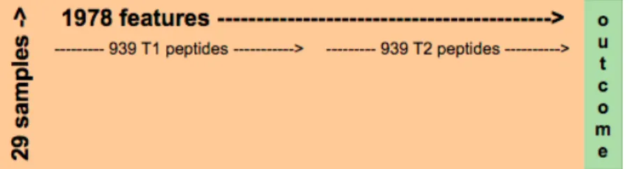
Figure 3.2: Pictorial representation of septic shock patient peptidome data after initial data preprocessing steps
Machine learning techniques will be used to analyse the dataset. From a ma-chine learning perspective the number of features of the data hugely outnumbers the number of samples (1878 vs 29). Furthermore, the dataset is typically imbalanced, with 23 survivors and 6 non-survivors.
1. T1 peptide abundances (939 peptide abundances) These peptides are labelled 0-938 in the following testing.
2. T2 peptide abundances (939 peptide abundances) These peptides are labelled 939-1877 in the following testing.
3. T1,T2 (T1_T2) peptide abundances (1878 peptide abundances) These are la-belled 0-1877, corresponding to the T1,T2 labelling.
NOTE: Peptide X observed in T1 is the same as peptide X+939 observed
at T2. The difference is whether it was found in T1 and T2. This is so that peptide abundances can be analysed independently in T1 and T2 and also considered together i.e. in T1_T2 data analysis, the same peptide observed at T1 and T2 is represented as two different features in the dataset.
(i) SMOTE
In general, learning models perform better with balanced classes to learn from. To combat the large class imbalance (Survivors:Non-survivors≈4:1), the data has been
over-sampled using Synthetic Minority Over-sampling Technique (SMOTE) [42]. The SciKit Learn implementation of imblearn.over_sampling.SMOTE was applied
to the original datasets for T1, T2 and T1_T2, creating datasets with balanced classes; 1:1.
The SMOTE algorithm generates new samples by looping through:
1. Consider an existing minority sample xi and identify its k nearest minority
class neighbours.
2. Choose one of its k neighbours at random, xj.
3. Synthesise a new sample on the line between the minority sample, xi, and the
chosen neighbour, xj, as follows:
x_new=xi+λ(xj−xi) (3.1)
where λ is a random number in the range [0, 1].
SMOTE-upsampled data was used for selecting features important for discriminating between classes. By oversampling in this way, models can sometimes better learn the patterns that separate classes. The SMOTE-upsampled data was not used by the classification algorithms, so the classifiers are being evaluated on original samples only.
(ii) Data transformations
The peptidome data is positively-skewed, with generally, a high frequency of low-values, this can be seen easily in Fig.3.3.
Of the 1,878 peptide abundance measures in T1 and T2, only 12 are normally dis-tributed. These are identified using SciPy.stats.normaltest for each peptide, which
tests whether a sample differs from the normal distribution, based on the skew and kurtosis.
Figure 3.3: Sample distributions of 3 T1 peptides chosen at random; (l-r) peptides 831, 238, 241
A number of different data transformations were tested to find the most appro-priate for the data. The data was log2, Box-Cox transformed and also discretised
into 10 bins. Thelog2 and Box-Cox transformations help by modelling proportional differences in abundance rather than additive, which is likely more relevant with this dataset. Of the 1,878 peptide abundances in T1 and T2, 12 of these are normally distributed. Afterlog2 and Box-Cox transformations, 1,200 and 1,193 are normally distributed, respectively. Similarly, discretising the data into 10 bins results in 1,254 normally distributed peptides. This transformation reduces the impact of noise and outliers in the data. All data transformations were used in the following testing, in order to identify if a certain transformation best suited the data. Ultimately, all transformations achieved very similar results andlog2 transformation was chosen as the most interpretable and easily understood in this domain.
3.2
Data Analysis
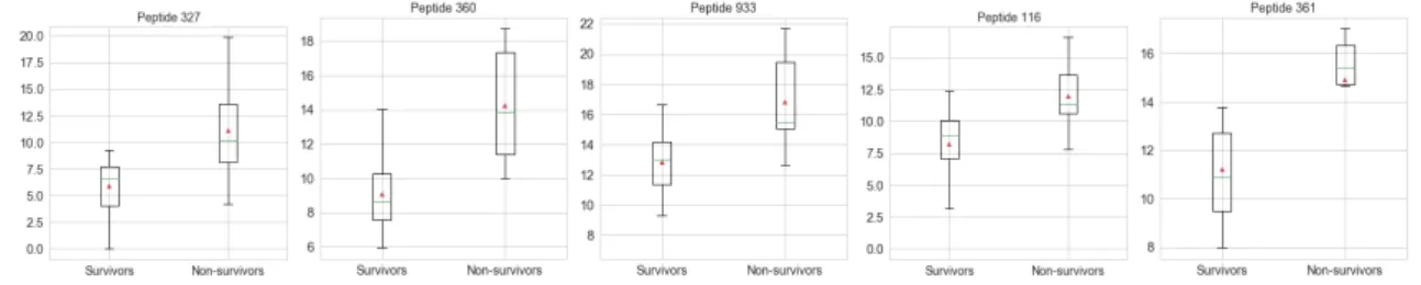
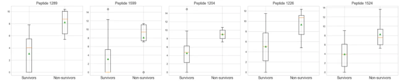
Initial statistics were calculated to better understand the data. The largest dif-ferences in T1 mean peptide abundance between S and NS patients were found in peptides shown in Fig.3.4, with their distributions. In every case we observe that the mean abundance is higher for NS than for S patients. Similarly, we see the same for T2; in the peptides with the 5 largest differences in mean abundance between S and NS patients, we observe that they occur in higher abundance in NS patients. This is observed in Fig.3.5.
Figure 3.4: Boxplots showing distribution of T1 (log2 transformed) peptides with biggest differences in mean abundance between survivors and non-survivors
Figure 3.5: Boxplots showing distribution of T2 (log2 transformed) peptides with biggest differences in mean abundance between survivors and non-survivors
4
|
Experiments
This chapter describes in detail the specific experiments that were undertaken as part of this thesis project, using the data described in Chapter 3. First, the experimental settings for feature selection, using feature importance of two ensemble algorithms, are included. The experimental settings for classification experiments follow, using the features selected by the ensemble algorithms. Three classification algorithms are described, including their parameters to be tuned. This is followed by a discussion of the metrics used to measure classifier success. The second half of the chapter comprises the results of these experiments and includes an in-depth discussion of them.
4.1
Experimental settings
4.1.1
Feature Importance
Two ensemble algorithms were used to identify feature importance in the data. En-semble methods are made up of a number of predictors which are combined (finding the average or most popular) to give the final prediction. This average of many pre-dictions is a better predictor than using just a single model. Ensemble methods can be described as bagging or boosting. In bagging, we construct independent models built using random subsamples of the data for each of the models. Each sample in the data has an equal chance of being used in each model. In boosting, each model is built independently, but sequentially, and the next model “learns” from the models before it. The samples that have the greatest errors are used most in order for the model to minimise its errors. Random Forest [43], an example of bagging, and XGBoost [44], an example of boosting were used to identify the most important (useful) peptides (features) in the classification of survivors/non-survivors.
Random Forest: The RF algorithm is an ensemble method made up of a num-ber of decision trees. In our implementation, the numnum-ber of trees was chosen to be 100 in order to achieve greater confidence and stability in the results without insurmountable execution times. For each tree, a random subset of samples is chosen, the sub-sample size is always the same as the original input i.e. 29 samples for original data and 46 for SMOTE data, but the samples are drawn with replacement. At each node, of each tree, a random subset of the features (in our implementation of size √n_f eatures, where n_f eatures
= 939 for T1/T2 or 1,878 for T1_T2) is used to decide the best split. Each tree is grown to the largest extent possible (max_depth = None). Finally, for
each observation, each tree ends with a probabilistic prediction of whether the patient will be a survivor or non-survivor. These values are averaged to choose
the predicted class. The relative importance of a feature with respect to pre-diction of the target variable is identified by its reduction in “Gini” impurity in the tree, and this is used to rank the features’ predictive power. The SciK-itLearn ensemble module was used for random forest implementation with the parameters fixed as:
n_estimators (trees) = 100 criterion = ’gini’ max_depth = None min_samples_leaf = 1 max_features = √n_f eatures random_state = 0-99
The features are randomly permuted at every node and therefore the best splits may vary. To ensure confidence and stability in our chosen features, the algorithm is run 100 times and the most important features over these 100 iterations are identified. To obtain deterministic behaviour, the random_state was set from 0 to 99 for each of the iterations. This ensures that the results can be reproduced.
RF analysis was carried out on the original datasets (for T1, T2, T1_T2), and also on the SMOTE up-sampled sets.
XGBoost: XGBoost (eXtreme Gradient Boosting) is an implementation of gra-dient boosted decision trees. It is currently acknowledged to be the favourite algorithm choice for Kaggle competition winners [45]. The boosting algorithm (like AdaBoost) is an ensemble technique where new models are sequentially added to predict and improve on existing errors, until no more improvements can be made. In XGBoost, a gradient descent algorithm is used to minimize the errors each time a new model is added; hence the name. The resulting en-semble of models is used for making the final prediction. The XGBoost library [46] was used to implement the gradient boosting decision tree algorithm. It includes many parameters which were fixed as the following:
num_round = 5 (This is the number of rounds (trees). It was found that 5 was
enough to ensure no further improvement in score).
eval_metric = ‘AUC’ (Area Under [the ROC] Curve; this was chosen to
evaluate the performance of the algorithm, as a good metric to use with im-balanced classes).
max_depth = 3 (Max depth of trees. This controls overfitting, as higher depth
allows model to learn samples very specifically).
eta = 1 (This is the learning rate).
max_delta_step = 1 (This controls the update of the weights and helps keep
them conservative).
scale_pos_weight= 3.8 (This controls the imbalance of the classes. #S/#NS
= 23/6 = 3.8)
and as our sample size is small, ensure all samples are used:
subsample: 1 (All samples are used in each tree).
colsample_bytree = 1: (All features are used in each tree).
Finally, the feature importances are measured by:
importance_type = ‘weight’
This means that features are ranked by the number of times they are used to split the data across all trees.
4.1.2
Classification
The following is implemented for all classification algorithms:
1) 5-fold Cross Validation (5-CV): The data is split into 5 stratified folds using SciKit Learn’s model_selection.StratifiedKFold implementation. 5-folds is chosen as
there are 6 NS samples and therefore not enough NS samples to have one in each of 10-folds. The random seed is set for these stratified folds (seed= 1,2,100). This
ensures that the same splits of data are tested with each classification algorithm and the results for each can be directly compared. We ensure that we can compare “like-for-like” with each machine learning algorithm, they are trained and tested on exactly the same data.
2) Leave-One-Out Cross Validaton (LOOCV): Additionally, the data is split using SciKit Learn’smodel_selection.LeaveOneOut()implementation. This
implemen-tation is useful with small sample size as the algorithm maximises the size of the training dataset, with which it learns with. Each training set is size n-1 (n=29 sam-ples), and each of the samples is tested once, with all other samples used to train the algorithm.
Logistic Regression
The first model used for classification was a traditional logistic regression model.
Algorithm: The SciKit Learn LogisticRegression class was implemented.
The model takes the sample inputs and predicts the probability that the sam-ple belongs to the default class, using the logistic function. If the probability is greater than 0.5 then the default class is chosen, otherwise the other class is chosen. The learning algorithm learns the best coefficients for the model using the training data, by a coordinate descent (CD) algorithm.
Advantage: Logistic regression functions well in the context of an unbalanced
outcome.
Parameters: C (Regularization penalty) was tuned to achieve optimal results
from C = {0.1, 1, 10, 100}. Smaller C values specify stronger regularization.
See Appendix for parameters used for each model. Support Vector Machine (SVM)
Algorithm: The SciKit Learn svm.SVC class was implemented. The model
uses a kernel function to transform the data and then a hyperplane is se-lected to best separate the points into their two classes. The coefficients of the hyperplane are found using an optimisation procedure (sequential minimal optimization).
Advantage: SVM are effective with high-dimensional data, including when the
number of features is larger than number of samples.
Parameters: kernel defines the kernel type. kernel = {‘linear’, ‘rbf’} were
tested to achieve optimal results. The ‘linear’ kernel is defined by the dot product between new samples and the support vectors hx, x0i. The ‘rbf’
kernel transforms the input space to a higher dimension. It is found by
exp(−γkx−x0k2).
gamma is the ‘rbf’ kernel coefficient. It defines the influence of a single training
sample. Larger gamma means the model tries to fit the training data more, which can lead to overfitting. gammawas tuned to achieve optimal results from gamma = {0.0001, 0.0005, 0.001, 0.005, 0.01}.
C controls the trade off between misclassifying training examples and
smooth-ness (simplicity) of decision boundary. Higher C aims to classify training
ex-amples correctly, with more complex (less smooth) decision boundary. C was
tuned to achieve optimal results from C = {1, 10, 100}.
See Appendix for optimal parameters used for each model. Multilayer Perceptron (MLP)
Algorithm: The SciKit Learnneural_network.MLPClassifier class was
im-plemented. MLP differs from logistic regression because between the input and output layers there can be one or more non-linear hidden layers. The MLP learns to represent the training data and how to best relate it to the output. It is made up of an input layer which passes the input to the hidden layer of (50 or 100) neurons. The summed weighted inputs to each neuron are passed through the (activation) rectified linear unit function (ReLu). In turn this passes to the output layer, made up of 1 neuron which uses a logistic activation function to output a value to represent the probability of predicting the default class. Starting from initial random weights, the MLP minimizes the cross-entropy loss function by repeatedly updating these weights. Our model was trained using Adam gradient descent optimizer. After calculating the loss, a backward pass propagates it from the output layer to the previous layers, updating each weight to decrease the loss. The algorithm stops when it reaches 1000 iterations; or when the improvement in loss is below 0.0001.
Advantage: Capability to learn non-linear models.
Disadvantage: Complex model which requires tuning of a number of
hyperpa-rameters.
Parameters: hidden_layer_sizes denotes the number of hidden layers and
number of neurons in each hidden layer. Increasing the number of layers and number of neurons increases the complexity of the model and the exe-cution time. In our model we tested only with 1 hidden layer, testing with
alphais the L2 regularization term which helps avoid overfitting by penalizing
weights with large magnitudes. alpha was tuned to achieve optimal results
from alpha = {0.1, 1, 10}.
See Appendix for optimal parameters used for each model. Metrics for measuring classifier performance
For each model, several metrics were evaluated to provide a more holistic mea-sure of overall performance. Due to the high proportion of S samples in the dataset (≈ 4:1), the accuracy of the model, alone, does not provide a clear indication of the
model performance. The following statistics were calculated:
1. ROC AUC
Area Under the Receiver Operating Characteristic Curve: The ROC curve is a useful technique to visualize the compromise between sensitivity and specificity for a classifier and the AUC summarizes ROC into a single value. This metric is useful because ROC curves are insensitive to class imbalance. The ROC AUC varies between 0 and 1, with an uninformed classifier returning 0.5. 2. Recall
Also the True Positive Rate (TPR) or sensitivity. This metric is particularly useful as correctly identifying the NS class is of high importance. It is calcu-lated by the following:
recall=tp/(tp+f n) (4.1)
where tp is the number of true positives and fn the number of false negatives.
Intuitively this is the ability of the classifier to identify all NS samples. A limitation of this metric is seen if no actual positives exist, and the metric is undefined. However, due to stratified sampling of the folds for testing, this will not be an issue.
3. Precision
Precision is a measure of exactness of the classifer. It is evaluated as the number of correct positive predictions, out of all positive predictions, using the following formula:
precision=tp/(tp+f p) (4.2)
where tp is the number of true positives and fp the number of false positives.
A limitation of this metric is seen if no positive predictions are made, then the equation is undefined and returns as 0 in our implementation.
4. F1
The F1 score is defined as the harmonic mean of precision and recall, it is a measure of the balance between the two metrics.
f1 = 2∗(precision∗recall)/(precision+recall) (4.3)
Similarly, this metric is undefined if no positive predictions are made, and our implementation returns a score of 0.
5. Specificity
Specificity is included to be able to see how well the classifier identifies Sur-vivors. It is found by:
Specif icity =tn/(tn+f p) (4.4)
wheretnis the number of true negatives andfp is the number of false positives.
The natural imbalance of the dataset indicates that more people are survivors than not, and this is the case in real-world scenarios. Therefore given the number of S patients, a small percentage of false alarms (false positives) would lead to a lower accuracy overall and this could discredit the classifier.
6. Accuracy
Accuracy is included for completeness, however the metric on its own does not describe well the quality of the classifier.
Accuracy= (tp+tn)/(tp+f p+tn+f n) (4.5)
i.e. the number of samples correctly classified, divided by the total number of samples.
TheKappastatistic will be calculated to help interpret more clearly the accu-racy scores of the models. The Kappa statistic describes how well a classifier model performs above the baseline model (of choosing the majority class only). It is found using:
kappa= (model accuracy−baseline accuracy)/(1−baseline accuracy) (4.6)
Most metrics described were implemented using the SciKit Learn metric class,
exceptSpecificity and kappa, which were calculated directly using their formulae given in above.
4.2
Experimental Results
4.2.1
Feature Importance
The important features were identified by 4 different models. 1. Random forest algorithm using original data
2. Random forest algorithm using SMOTE-upsampled data 3. XGBoost algorithm using original data
4. XGBoost algorithm using SMOTE-upsampled data
The random forest algorithm identifies all features that it believes to be useful in discriminating between classes, by its reduction in “Gini” impurity in the tree. The top 50 features (peptides) were chosen from those with a feature_importances_ score≥0. The mean number of features identified with feature importance greater
than 0, for T1 original (not-SMOTE) data was 192, for T2 it was 195, and for T1_T2 it was 202 features. The XGBoost algorithm, however, identifies relatively few important features. Using the same data the algorithm found 8 features important from T1, T2 and T1_T2. This could be because we have many correlated features within our data. When the XGBoost algorithm chooses a feature, it might use this feature in many trees (learnt sequentially) and any correlated features will not be used, as they do not add any additional information. Instead, the RF algorithm chooses features randomly for each tree, done in parallel, and may choose different, correlated features for each new tree.
T1
361 : IAALLSPYSYSTTAVVTNPKE was found to be the most important peptide by all 4 models. This peptide was found to have one of the top five biggest differences in mean abundance between NS and S samples, in our earlier data anal-ysis.
Additionally, 2 more peptides were found to be important by all 4 models: 427 : KTETQEKNPLPSKETIEQEKQAGES
1 : AAEVISNARENIQ
The XGBoost algorithm agreed on 5 features (out of 8 and 7) based on original and SMOTE data:
361 : IAALLSPYSYSTTAVVTNPKE 1 : AAEVISNARENIQ
10 : AEDSLADQAANKWGRSGRDPNH 427 : KTETQEKNPLPSKETIEQEKQAGES 750 : SSKITHRIHWESASLLR
The RF algorithm agreed on 28 features (out of 50 for each) based on the original and smote data. See appendix A for full list of 50 peptides identified.
T2
1204 : FSPSVVHLGVPLSVGVQLQDVPRGQVVKGSVFwas found to be
the most important peptide by 3 out of 4 models, and 2nd most important by the 4th model. This peptide was found to have one of the top five biggest differences in mean abundance between NS and S samples, in our earlier data analysis.
Additionally, 1 more peptide was found to be important by all 4 models: 1111 : EESNYELEGKIK
The XGBoost algorithm agreed on 3 features (out of 8 and 7) based on original and SMOTE data:
1204 : FSPSVVHLGVPLSVGVQLQDVPRGQVVKGSVF 1111 : EESNYELEGKIK
939 : AAEAISDARENIQ
peptides.
The RF algorithm agreed on 21 features (out of 50 for each) based on the original and smote data. See appendix A for full list of 50 peptides identified.
11 T2 peptides identified as important by the random forest algorithm were also identified as important in T1. These include EESNYELEGKIK (found important by all models in T2; key:1111) and KTETQEKNPLPSKETIEQEKQAGES (found important by all models in T1; key:427).
T1_T2
This data includes all abundance measures of peptides at both times, T1 and T2. This is therefore the most comprehensive (and complex in terms of dimensionality) dataset.
1204 : FSPSVVHLGVPLSVGVQLQDVPRGQVVKGSVF (the most
important peptide from T2) was also deemed to be the most important from data including T1 and T2, for 3 out of the 4 models, and 2nd most important for the 4th model.
Additionally, 1 more peptide (from T2) was found to be important in all 4 mod-els:
1111 : EESNYELEGKIK
The XGBoost algorithm agreed on 4 features (out of 8 and 9) based on original and SMOTE data:
1204 : FSPSVVHLGVPLSVGVQLQDVPRGQVVKGSVF
45 : ALTLTKAPADLRGVAHNNLMA (was not chosen as important by XGBoost using just T1 data)
1111 : EESNYELEGKIK
361 : IAALLSPYSYSTTAVVTNPKE
Of the 13 unique features identified by both XGBoost algorithm models, from the T1 and T2 data, only 4 were identified as important in separate T1 and T2 data. These are the peptides with keys: 1204, 1111, 1802, 361. Of the 9 “new” peptides identified, 8 were T1 peptides.
The RF algorithm agreed on 24 features (out of 50 for each) based on the original and smote data. Of the 76 unique peptides identified by both random forest models, from the T1 and T2 data, only 1 was not identified in separate T1 and T2 data. See appendix A for full list of 50 peptides identified.
4.2.2
Classification using Important Features
Baseline classification model
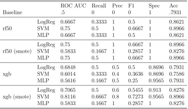
The chosen metrics are evaluated for the baseline model and shown in 4.1. The baseline classification model is defined by classifying all samples as the majority
class (0/Survivor). Due to the high class imbalance in this dataset, a high accuracy score of 0.7931 is obtained using this baseline model. The kappa statistic is a measure of improvement of the model on this baseline and therefore is 0. The recall, precision and F1 scores evaluate the ability of the model to identify the Non-survivor (NS) class and exactness of the NS class predictions. The baseline model does not identify the NS class by definition, and therefore baseline recall, precision and F1 scores are 0. The ROC AUC metric returns a score of 50%, which indicates that this model is an uninformed classifier. The specificity is a measure of how well the model classifies the survivor class, so by definition of the baseline model, this score is 1.
ROC AUC Recall Precision F1 Specificity Accuracy Kappa
0.5 0 0 0 1 0.7931 0
Table 4.1: Baseline metrics results
T1 Discussion
The results based on peptides taken at T1, i.e. 16 hours after shock first diag-nosed, illustrate various degrees of success for classification of patient outcome. The best classification results for T1, considering all metrics, are achieved using a SVM classifier on the top features found with SMOTE-upsampled data by the XGBoost algorithm. These results can be seen in Table 4.2, highlighted in bold. A recall rate of 0.7222 is achieved, indicating that 72% of all the NS are correctly classified. A specificity score of 0.9565 indicates that less than 5% of S samples are misclassified i.e. S classified as NS. Furthermore, the overall accuracy of this model is 90.8% (approximately 10% higher than baseline), which equates to akappa value of 0.56.
In general, the models were able to more easily successfully classify S samples than NS samples. This is intuitive as there is a large bias in the size of classes, with 79% S samples, and therefore the model has more data to better learn the S class. Each of the 12 permutations of models tested achieved a specificity (ability to predict S) rate≥92%. However, the recall rate (ability to predict NS) was as low as 11%, and
the average recall rate was 40%. This demonstrates the difficulty for the models to learn to classify NS patients, from a very small number of samples (n=6).
T2 Discussion
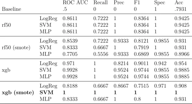
The classification models using the most important features found in T2 data were largely successful. The best result was found using the best features obtained by the XGBoost algorithm with SMOTE-upsampled data, and SVM classifier (as in T1). This result, shown in bold in Table 4.6, achieved 100% for all metrics. We observe, generally, that the XGB features achieved better results overall than the RF chosen features. This could be because of the number of features chosen. Using the RF algorithm, the best 50 features were included. However, 50 features may still be too many features for the optimisation of our classification algorithms.
It is worth observing in Table 4.4 that 4 models achieved 100% recall score of NS samples. Three of these 4 models were the three classifiers using the XGBoost
ROC AUC Recall Prec F1 Spec Acc Baseline .5 0 0 0 1 .7931 rf50 LogReg 0.6667SVM 0.7283 0.33330.5 10.75 0.50.6 10.9565 0.86210.8621 MLP 0.6667 0.3333 1 0.5 1 0.8621 rf50 (smote) LogReg 0.715SVM 0.6111 0.44440.2222 0.88891 0.59260.3571 0.98551 0.87360.8391 MLP 0.7222 0.4444 1 0.6111 1 0.8851 xgb LogReg 0.6993SVM 0.686 0.50.4444 0.56670.7 0.53030.5152 0.89860.9275 0.81610.8276 MLP 0.5556 0.1111 0.6667 0.1905 1 0.8161 xgb (smote) LogReg 0.7415 0.5556 0.6667 0.6061 0.9275 0.8506 SVM 0.8394 0.7222 0.8111 0.7626 0.9565 0.908 MLP 0.5761 0.1667 0.8333 0.2738 0.9855 0.8161 Table 4.2: T1 mean 5-fold CV classification results, using features selected by RF algorithm (best 50 features: rf50) and XGBoost algorithm (xgb)
(non-SMOTE) chosen features. Therefore, using these features (peptides), it ap-pears that a classifier is able to identify all NS samples and so these peptides could be important in further exploration as indicators of NS patient outcome. In addi-tion, these models would be good choices if it is most important to identify patients with high risk of death, although this may be done with a bias towards the NS class meaning others may be wrongly classified (false-positives).
Features used to classify patient outcome with 100% accuracy
Our SVM classifier is able to classify patient outcome with 100% accuracy using the T2 features (peptides) obtained using XGBoost algorithm on SMOTE-upsampled data. Analysing the SVM coefficients, we can identify which features (peptides) are used to classify the data as Non-survivors and Survivors and also their relative importance, shown in Fig.4.1. We see from this plot that the following peptides are used by the classifier to achieve 100% correct classification, listed in order of importance: 1. 1204 : FSPSVVHLGVPLSVGVQLQDVPRGQVVKGSVF (=> NS) 2. 1289 : HPNSPLDEENLTQEN (=>NS) 3. 976 : ALEEQLQQIRAE (=>S) 4. 1111 : EESNYELEGKIK (=>NS) 5. 1226 : GAGGEDSAGLQGQTLTGGPIRIDWED (=> NS) 6. 1066 : DLSTPDAVMGNPKVKA (=> S) 7. 939 : AAEAISDARENIQ (=> NS)
ROC AUC Recall Prec F1 Spec Acc Baseline .5 0 0 0 1 .7931 rf50 LogReg 0.6667SVM 0.75 0.3333 10.5 1 0.50.6667 11 0.86210.8966 MLP 0.6667 0.3333 1 0.5 1 0.8621 rf50 (smote) LogReg 0.75SVM 0.5833 0.50.1667 11 0.6667 10.2857 1 0.89660.8276 MLP 0.75 0.5 1 0.6667 1 0.8966 xgb LogReg 0.6848SVM 0.6014 0.50.3333 0.40.5 0.50.3636 0.8696 0.75860.8696 0.7931 MLP 0.5616 0.1667 0.5 0.25 0.9565 0.7931 xgb (smote) LogReg 0.7065SVM 0.8116 0.50.6667 0.80.6 0.5455 0.9130.7273 0.9565 0.89660.8276 MLP 0.5833 0.1667 1 0.2857 1 0.8276 Table 4.3: T1 LOOCV classification results, using features selected by RF algorithm (best 50 features: rf50) and XGBoost algorithm (xgb)
Figure 4.1: T2 SVM coefficients
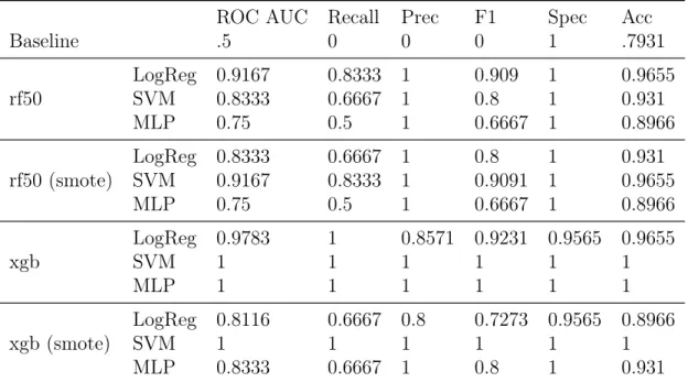
Taking a look at the boxplot distributions for NS and S patients for each of these peptides, in 4.2 we see that for each, they are remarkably different, which is presumably why they are important for classifying patient outcome. We show the peptides used to help classify NS samples in the top row of the figure, in order of importance. We notice the top 4 peptides are in noticeably higher abundance for NS patients. On the contrary, shown together in the bottom row, we see the 2 peptides that help to classify S samples have higher abundance for S patients.
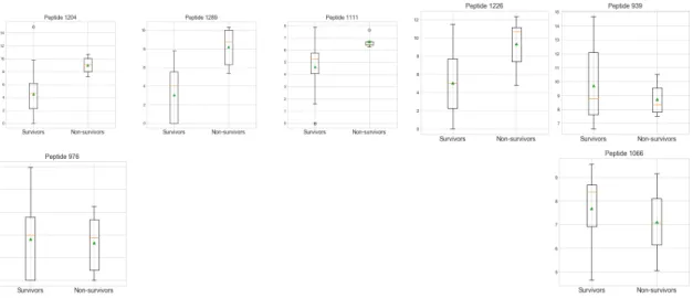
Furthermore, in Fig.4.3 we observe that if we plot the abundances of the top 3 of these “important” peptides for classifying samples, i.e. 1204, 1289 & 976, we see that the six NS patient samples are plotted in the same region, i.e. they are potentially separable from the S samples. We also observe this result when we plot the same for the top 3 peptides used to classify NS samples, i.e. 1204, 1289, 1111. These results are intriguing, and contribute to the conclusion that these peptides alone could be used to predict patient outcome.
ROC AUC Recall Prec F1 Spec Acc Baseline .5 0 0 0 1 .7931 rf50 LogReg 0.8611SVM 0.8611 0.7222 10.7222 1 0.8364 10.8364 1 0.94250.9425 MLP 0.8611 0.7222 1 0.8364 1 0.9425 rf50 (smote) LogReg 0.8539SVM 0.8333 0.7222 0.9333 0.8121 0.9855 0.9310.6667 1 0.7919 1 0.931 MLP 0.7705 0.5556 0.9333 0.6869 0.9855 0.8966 xgb LogReg 0.971SVM 0.9928 11 0.8214 0.9011 0.9420.9524 0.9744 0.9855 0.98850.954 MLP 0.9928 1 0.9524 0.9744 0.9855 0.9885 xgb (smote) LogReg 0.8188 0.6667 0.8667 0.7515 0.971 0.908 SVM 1 1 1 1 1 1 MLP 0.8333 0.6667 1 0.8 1 0.931
Table 4.4: T2 mean 5-fold CV classification results, using features selected by RF algorithm (best 50 features: rf50) and XGBoost algorithm (xgb)
Finally, in Fig.4.4 we include a heatmap plot of the abundances of the peptides used to classify patient outcome with 100% accuracy, for all patients. For ease of visual understanding, the S patients are the top 23 rows of the heatmap and the NS patients are the bottom 6. It is useful to compare the variations in abun-dances for each peptide. We notice that there are some clear examples where the abundances for the last 6 rows are quite different from the others. In general, this is mostly true for peptides 1204, 1289 (the top 2 most important peptides) and 1226.
Features used to classify patient outcome with 99% accuracy
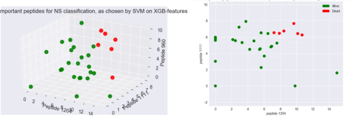
We also take a closer look at our model that achieved 99% accuracy, which is still an exceptional result. The model used the peptides selected by XGBoost algorithm (using not-SMOTE-upsampled data) and a SVM classifier. There were 8 peptides selected by XGBoost, of which, 3 are the same as our other ‘best’ model. We bet-ter analyse the use of these peptides in our classification model by obtaining and plotting the SVM coefficients, shown in 4.5. We find the same result in this model: peptide 1204 is the most important for classification. Peptide 1111 is the next most important, this is also used in our 100% model. We plot 4.6 the abundances of the top 3 peptides from this model: 1204, 1111, 960 and observe again that our samples are visually separable. Furthermore, we plot just the top two peptides: 1204 vs 111; and we observe the NS and S samples are clearly grouped and again visually separable. This is an interesting result that indicates that these two peptides alone could provide a lot of information regarding septic shock prognosis.
T1_T2 Discussion
We observe in Tables 4.7 and 4.8 that our classification results using peptides from T1 and T2, are better than for T1 peptides but less successful than classifiers using
ROC AUC Recall Prec F1 Spec Acc Baseline .5 0 0 0 1 .7931 rf50 LogReg 0.9167SVM 0.8333 0.8333 10.6667 1 0.9090.8 11 0.96550.931 MLP 0.75 0.5 1 0.6667 1 0.8966 rf50 (smote) LogReg 0.8333SVM 0.9167 0.6667 10.8333 1 0.80.9091 11 0.9310.9655 MLP 0.75 0.5 1 0.6667 1 0.8966 xgb LogReg 0.9783SVM 1 11 0.8571 0.9231 0.9565 0.96551 1 1 1 MLP 1 1 1 1 1 1 xgb (smote) LogReg 0.8116SVM 1 0.6667 0.81 1 0.7273 0.9565 0.89661 1 1 MLP 0.8333 0.6667 1 0.8 1 0.931
Table 4.5: T2 LOOCV classification results, using features selected by RF algorithm (best 50 features: rf50) and XGBoost algorithm (xgb)
T2 peptides only. Like our T2 classifiers, the results improve when using the XG-Boost chosen features over the RF 50 top features. The result with highest mean accuracy for 5-fold CV was achieved using the XGBoost chosen features (original, not up-sampled data), with a logistic regression classifier. The classifier averaged 94% successful classification of NS samples, and 100% of S samples. The average accuracy achieved was 98.85%, which equates to a kappa score of 94%. The SVM classifiers, using the same data and the SMOTE-upsampled xgb data, obtain 100% recall scores i.e. all NS samples are identified, and overall accuracy is just slightly lower, 96.55% and 97.7% respectively.