Using information theoretic measures to evaluate support vector machine kernels

c

USING INFORMATION THEORETIC MEASURES TO EVALUATE SUPPORT VECTOR MACHINE KERNELS

BY

AUSTIN PIERCE

THESIS

Submitted in partial fulfillment of the requirements

for the degree of Master of Science in Electrical and Computer Engineering in the Graduate College of the

University of Illinois at Urbana-Champaign, 2012

Urbana, Illinois Adviser:

ABSTRACT

A new method is proposed that exploits the underlying information theoretic structure in the input data to evaluate the ability of a kernel to successfully separate a class in some feature space. This method is built on the funda-mental idea that kernel density estimation in some input space is equivalent to an inner product on some Hilbert space. Estimators of R´enyi’s general-ized form of information theoretic measurements reduce to a form that gives an elegant characterization of the geometric properties of the kernel in the feature space. It is shown how these estimators can be used to evaluate the kernel of a support vector machine.

But I have promises to keep, And miles to go before I sleep, And miles to go before I sleep.

ACKNOWLEDGMENTS

I think this is as close as I will ever get to a Grammy speech. First, I want to thank my parents for their never ending support, love, and guidance. Without them I would not be half the person I am today. This paper is dedicated to them. To my sister for constantly reminding me that hard work also requires hard play. You only live once, YOLO.“I don’t care how poor a man is; if he has family, he’s rich.”

I would like to thank Science Applications International Corporation (SAIC) for giving me the opportunity to work four summers alongside some of the smartest people I have ever met. The experience I have gained working there is invaluable and completely transformed how I approach engineering. This thesis would not have been possible without the conversations I had with Mike Tinston.

I am thankful to Prof. Richard Blahut for accepting me into his research group and for providing insightful weekly meetings.

TABLE OF CONTENTS

CHAPTER 1 INTRODUCTION . . . 1

1.1 Machine Learning . . . 1

1.2 Learning Model . . . 4

1.3 Motivation . . . 6

CHAPTER 2 INFORMATION THEORY . . . 8

2.1 Shannon Entropy . . . 8

2.2 R´enyi Entropy . . . 11

2.3 R´enyi Entropy vs. Shannon Entropy . . . 13

2.4 Quadratic R´enyi Entropy . . . 14

2.5 Cauchy-Schwarz Divergence . . . 17

CHAPTER 3 REPRODUCING KERNEL HILBERT SPACES . . . . 19

3.1 RKHS Definitions . . . 19

3.2 Density Estimation and RKHS . . . 21

CHAPTER 4 SUPPORT VECTOR MACHINES . . . 24

4.1 Vapnik-Chervonenkis Theory . . . 24

4.2 Support Vector Machine . . . 25

4.3 Kernel Trick . . . 28

4.4 Evaluating Kernels Using Information Theory . . . 29

CHAPTER 5 CONCLUSION . . . 32

CHAPTER 1

INTRODUCTION

The decision-making process behind identifying or classifying objects is often associated with the recognition of patterns. For example, determining the context and language of handwritten characters, using facial structure to detect individuals in photos, and deciding whether or not to buy or sell a stock based on current and past market trends. Recognizing patterns, collecting raw data, or making an action based on specific features of the input is a complex process that the human mind manages on a daily basis. For this reason, the creation of machines capable of learning patterns has been a popular research topic both from a technical and philosophical perspective. Technological advances in computer processing have allowed machines to demonstrate a significant ability to learn and recognize patterns. However, in order to demonstrate these tasks using classical programming techniques, there must be some foundation for the mathematical model of the problem. The methodology and theory behind the mathematical approach has formed the foundation for machine learning.

1.1

Machine Learning

Artificial intelligence is the term coined to describe the capability of ma-chines to mimic and simulate intelligent human behavior. Machine learning has evolved as a branch of artificial intelligence that is concerned with under-standing how to give machines the ability to learn and analyze data to make intelligent decisions. When computers are applied to solve a problem, they all follow the same practical architecture. The input data is fed through some system and mapped to an output. It is up to the system designer to develop a method for implementing the relationship between the input/output pairs. However, in some cases the relationship is not explicit, constantly

chang-ing, or the relationship is so complex that the computation is too expensive. When the problem or relationship is too complicated, the system designer cannot always implement a method for computing the output from the input data using classical programming techniques. The alternative method is to develop a system capable of learning or recognizing the pattern between the input and output based on examples, or given some specific criterion.

Learning in this context is achieved using mathematical principles. The framework is built on inductive inference; that is, observing samples that may or may not completely represent the input and predicting the output [1]. Generally, the input and output are related through some kind of dependency. When the dependency exists, it is referred to as the environment operator. The goal of the machine is to learn, and according to some cost, estimate the environment operator. The estimate is often referred to as the decision operator or classifier. Because the environment is not always completely understood, the decision operator is often chosen from a particular set or class of hypothesis operators. The learning process is simply choosing the appropriate operator, or classifier, from the class of hypothesis operators that best represents the environment operator.

Any method that attempts to describe the environment operator according to some prior knowledge employs learning. While learning follows a general model, it is the specific method used that determines the unknown parame-ters of the model and the structure of the classifier. Ideally, the classifier will generalize well to new patterns and data. How well the classifier performs on new data is referred to as generalization, and is the property that we seek to optimize. This framework results in two general forms of learning: supervised learning and unsupervised learning.

1.1.1

Supervised Learning

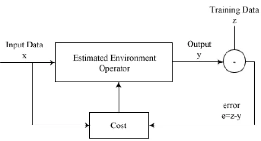
Supervised learning is primarily concerned with the identification of func-tional dependencies between the input xi and output zi. The environment operator is assumed to be some kind of functional mapping that is estimated from pairs of samples (xi, zi) called the training data. Figure 1.1 shows the basic framework for a supervised learning system. The dataxi is fed through the estimated environment operator to produce an output yi. The outputyi

Figure 1.1: A basic supervised learning system.

is then compared to zi to produce an error signal. The error signal is used to systematically update the environment according to some cost criterion. Over time the system will adapt the estimated environment operator so that the data xwill produce a y that will approximate z.

A classifier that accurately fits the training data is said to be consistent. Generating consistent classifiers raises important issues. In cases where the output is noisy, there is no guarantee that a functional mapping exists. So, the classifier has to be implemented optimizing some best-fit criteria. If the classifier is designed to be too complex, it is possible to overfit the data. When this occurs, the classifier may correctly separate the training samples but will fail to generalize well to new data. In supervised learning, the design is concerned with optimizing the tradeoff between accuracy and reliability.

1.1.2

Unsupervised Learning

The goal of unsupervised learning is to capture regularities and statistical dependencies between the input xi and output yi. An unsupervised system follows the same framework as the supervised system in Figure 1.1 only x

is available but z is not. The environment operator is assumed to function according to a set of specifications. The function is typically controlled by a cost. The classifier is designed to use the cost to form clusters or groupings of

the input. The output yi from the classifier is entirely dependent on the cost that is implemented to replicate the environment operator. In unsupervised learning the design is primarily concerned with optimizing the cost to create a classifier that appropriately represents the regularities of the input data.

1.2

Learning Model

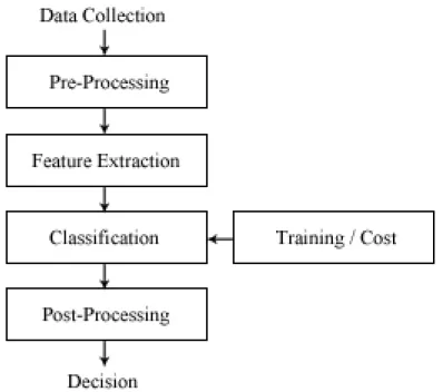
Now that we have introduced the foundation for machine learning, we can start to develop the systematic model for implementation on a computer [2]. Figure 1.2 shows the typical layout and components of a machine learning system. Understanding the importance of each component will clarify the problems with designing such a system and establish the motivation behind this research.

1.2.1

Data Collection

Data is typically collected using some kind of transducer, such as a micro-phone or sensor. The limitations and characteristics of the transducers, such as the signal-to-noise ratio or distortion, are often part of the problem. These limitations feed through the system and can affect each component if they are not considered in the design process. The amount of data that is collected and processed can significantly constrain other components, especially if the system is expected to work in real-time.

1.2.2

Pre-Processing

The data that is collected by the transducer is typically referred to as raw data. The raw data is often noisy, disorganized, or not in a format capable of being processed by the rest of the system. The purpose of the pre-processor is to prepare the raw data for feature extraction. Often this requires some kind of filtering or grouping operation. Ideally the pre-processor will isolate specific idiosyncrasies in the data.

1.2.3

Feature Extraction

The purpose of the feature extractor is to find distinguishing properties in the data that can be used to characterize an object or class. These distinguishing features are what the classifier will use to isolate the input and predict the output. When choosing these features, it is important that they are invariant to irrelevant transformations. For example, the data could get scaled or rotated in the pre-processing stage. If the distinguishable feature is affected by one of those transformations, then the feature will make it difficult for the classifier to reliably separate the input. The feature extractor is entirely domain-dependent. An extractor that successfully characterizes one problem will not necessarily work well for another.

1.2.4

Classification

The classifier is the most important component of the system and the most complicated. Because perfect classification is often impossible, the

classi-fier is built on a probabilistic framework. The general task is to use the distinguishing features to assign the input to a group or category with the smallest probability of error. The design is application dependent and fol-lows one of the two general forms of learning: supervised or unsupervised. In the supervised case the classifier is fed training data to estimate a functional relationship between the input and output. In the unsupervised case the classifier is given a cost or criterion to group the output based on statistical dependencies of the input. The difficulty behind designing the classifier of-ten depends on the size of the feature space and the difference between the distinguishing features in different categories. If the distinguishing features are drastically different, then the classifier dramatically simplifies. However, if the features are similar or if they are very noisy, the classifier can become much more complex.

1.2.5

Post-Processing

While the classifier analyzes the distinguishing features and classifies the data, it is up to the post-processor to decide the final action. Typically the post-processor is used to tweak the output of the classifier and improve system performance. This modification can be as simple as filtering the data to reduce output noise, or as complicated as regularizing the output to meet some specification.

1.3

Motivation

While it is not necessarily obvious, it should be relatively straightforward to notice that the problems and difficulties in designing each component can be manipulated in the classifier. For example, the amount of data collected during the collection stage is irrelevant if the classifier is capable of handling large amounts of data. Likewise, the variation in the distinguishable features can be changed if the classifier takes advantage of some kind of transfor-mation. For this reason, this thesis will focus entirely on the design of the classification component of the learning model. Recall that the classifier is designed according to one of the two general forms of learning: supervised or unsupervised. Supervised learning requires the estimation of some

func-tion to mimic the environment operator, and unsupervised learning attempts to find the statistical dependency in the input data. So the classifier is in-herently built on a probabilistic framework. While a Bayesian or maximum likelihood approach is reasonable and well understood, a new question is proposed: Are there other well-established probabilistic theories that can be used to take advantage of the statistical properties of the input? If so, what advantages does it provide? As it turns out, the answer lies in the field of information theory. Specifically, in R´enyi’s generalization of information the-ory. We will show that it is possible to evaluate how well a kernel function separates data in some feature space using information theoretic estimations on the input data. This method is built on the fundamental idea that kernel density estimation in some input space is equivalent to an inner product on some Hilbert space. Estimators of R´enyi’s generalized form of information theoretic measurements reduce to a form that gives an elegant characteriza-tion of the geometric properties of the kernel in the feature space. We apply this kernel evaluation to the design of a Support Vector Machine.

This thesis is organized as follows. In Chapter 2 we introduce the idea of

αth-order information theoretic measures and their estimators. We develop the foundation for reproducing kernel Hilbert spaces in Chapter 3 to help form an important geometric understanding of these measures. In Chap-ter 4 we introduce the Support Vector Machine and propose a method for evaluating the feature spaces of kernels using information theory. We make concluding remarks and offer further research ideas in Chapter 5.

CHAPTER 2

INFORMATION THEORY

Information theory was originally conceptualized by Shannon to help estab-lish the fundamentals behind data compression and transmission rates in communication systems [3]. For this reason, information theory is often con-sidered to be a branch of communication theory. However, the probabilistic framework has laid the foundation for contributions in other areas of math and the sciences [4]. We introduce information theoretic measurements here as a probabilistic reasoning method for analyzing the statistical properties of data. Keep in mind that the motivation behind doing this is to exploit these statistical descriptors as tools when designing a classifier. We will start by introducing the original ideas developed by Shannon and explain the purpose of entropy, divergence, and mutual information. This will lead to a general-ized form of information theory developed by R´enyi. We will show that the estimator for R´enyi entropy reduces to a form that is easier to compute than Shannon entropy.

2.1

Shannon Entropy

In 1928 Hartley introduced the first quantitative measure of information. He defined this information as the number of choices in a finite set of possible symbolsS[5]. According to Hartley, the amount of information in a sequence of N symbols could be quantified as I = log_bSN. If the logarithm is base ten, then we refer to the unit as a Hartley. In the digital age we prefer to think in terms of binary symbols [0,1], so the logarithm is taken to the base two and is referred to as the bit.

It was Shannon who went a step further and introduced the idea that the information content was dependent on the probabilities of the symbols. Let us define a random variable X with a finite set of possible outcomes

X = {x1, . . . , xN} having a probability mass function p(x) = Pr{X = x},

x∈ X. Shannon first showed that Hartley’s information was only accurate if nothing was known about the distribution of the symbols; that is, we assume that the symbols occur with equal probability p(x) = _{|X |}1 . Thus, in order to fully characterize the amount of information for each element xk in X, the information should be I(xk) = log 1 p(xk) =−log₂p(xk). (2.1) .

The amount of information in a specific event is due to the inverse depen-dence on probability. If N = 1, then p(x1) = 1 and the information content

I(x1) is zero. This means we have perfect knowledge of the event since we know there is only one possible event outcome. Likewise, if N is large and

p(x) is small, then the information content is high because the event is unex-pected. To describe the information or uncertainty over the set of outcomes X, Shannon defined entropy as the average of the information measure over each event, or H(X) = X x∈X p(x)I(x) =−X x∈X p(x) log₂p(x) = −E[log₂p(x)]. (2.2) Shannon’s entropy provides a single scalar quantity that describes the un-certainty underlying the probability mass function (PMF). In other words,

H(X) depends on the shape of the distribution. It is not the only scalar quantity that describes the PMF; for example, the mean and variance are also widely used. However, entropy provides a deeper insight into probabilis-tic reasoning because of its elegant properties. Shannon proved and built his definition of entropy on a set of simple axioms [3]:

1. H(p(x))≥0 ∀ x∈ X.

2. H(p(x1), p(x2), . . . , p(xN)) is a continuous and symmetric function of its arguments.

3. H(_N1,_N1, . . . ,_N1) is a monotonically increasing function ofN.

4. H(p(x1), p(x2)) =H(p(x1)) +H(p(x2)) for independent events x1 and

5. H(p(x1), p(x2), . . . , p(xN)) =H(p(x1)+p(x2), p(x3), . . . , p(xN))+(p(x1)+

p(x2))H(_{(p(x1)+p(x2))}p(x1) ,_{(p(x1)+p(x2))}p(x2) ), entropy is recursive.

Shannon proved that Equation (2.2) was the only solution forH(X) that satisfied the above axioms. It is important to note that H(X) is upper bounded by the Hartley information, H(X) ≤ log|X |. As it turns out, entropy is a concave function [4] which makes it susceptible to a large area of mathematics.

2.1.1

Other Information Measurements

Entropy is only concerned with describing the uncertainty of a single source of information. However, communication systems have inputs and outputs, just like a learning machine. To characterize the relationship between two differ-ent information sources, Shannon’s theory led to two well-known descriptors called the Kullback-Leibler (KL) divergence and mutual information. Con-sider the discrete random variable X with a finite set of possible outcomes X ={xk}Nk=1. Let p(x) and q(x) be two probability mass functions defined on X. Then the KL divergence is defined as

DKL(p||q) = X x∈X p(x) logp(x) q(x) =Ep logp(X) q(Y) . (2.3)

The KL divergence is a way to measure how close the distribution q is to p. When p=q the KL divergence is zero. However,DKL(p||q)6=DKL(q||p), so it is not a true measure of distance.

Now let Y be a random variable with a finite set of possible outcomes Y ={yk}Nk=1. Let the joint probability mass function between X and Y be

p(x, y) and the marginal probability mass functions be p(x) and p(y). Then the mutual information between X and Y is

I(X;Y) =X x∈X X y∈Y p(x, y) log p(x, y) p(x)p(y) =Ep(x,y) log p(X, Y) p(X)p(Y) . (2.4)

The mutual information measures the amount of information that one ran-dom variable contains about another. Mutual information can also be written

in terms of the KL divergence as

I(X;Y) =DKL(p(x, y)||p(x)p(y)). (2.5) Thus, it is also possible to think of mutual information as measuring how close X and Y are to being independent.

2.2

R´enyi Entropy

In 1960 Alfr´ed R´enyi was searching for a general definition of information the-oretic measures that would preserve the additivity property for independent events. He started with the probabilistic view of Hartley’s information in Equation (2.1) since it was already shown by Shannon that this was required to preserve the additivity property. He recognized that the total amount of information developed by Shannon,

H(X) = X x∈X

p(x)I(x), (2.6) assumed that the average was linear. Instead of assuming a linear relation-ship, he decided to apply the general theory of means. For any monotonic and continuous function g(x), the general form of the mean applied to Equation (2.6) is H(X) =g−1 " X x∈X p(x)g(I(x)) # . (2.7)

R´enyi showed that only two possible functions satisfied Equation (2.7) with the additive property [6]. One possible function was g(x) =cx, which is just a linear function and reduces Equation (2.7) to Shannon entropy. The other function was g(x) =c−2(1−α)x, which when applied to Equation (2.7) implies

Hα(X) = 1 1−αlog X x∈X pα(x) (2.8)

where α 6= 1 and α ≥ 0. Equation (2.8) is a parametric family of functions that is referred to as the αth-order R´enyi entropy.

L’Hˆospital’s rule, we see that lim α→1Hα(X) = limα→1 1 1−αlog X x∈X pα(x) (2.9) = limα→1 P x∈Xpα(x) logp(x) P x∈Xpα−1(x) limα→1−1 (2.10) =−X x∈X p(x) logp(x). (2.11) Shannon entropy can be determined by R´enyi entropy when α is near 1. Thus, Shannon entropy is just a member of the class of R´enyi entropies. For this reason, R´enyi entropy is often referred to as a generalized form of Shannon entropy.

2.2.1

Information Measurements of Degree

α

Following Shannon’s theory, R´enyi also developed measurements to describe the relationship between two information sources. Consider the discrete ran-dom variable X with a finite set of possible outcomesX ={xk}Nk=1. Letp(x) and q(x) be two probability mass functions defined on X. Then the R´enyi

α-divergence is defined as [6] Dα(p||q) = 1 α−1log X x∈X p(x) p(x) q(x) α−1 . (2.12)

By taking the limit as α approaches one and applying L’Hˆospital’s rule, it is easy to see that Equation (2.12) approaches the KL divergence in Equation (2.3): lim α→1Dα(p||q) = limα→1 1 α−1log X x∈X p(x) p(x) q(x) α−1 (2.13) = −limα→1 P x∈Xp(x) _p(x) q(x) α−1 logq(x)_p(x) limα→1 P x∈X p(x) q(x) α−1 (2.14) =−X x∈X p(x) log q(x) p(x) (2.15)

=X x∈X

p(x) log p(x)

q(x) =DKL(p||q). (2.16) Now let Y be a random variable with a finite set of possible outcomes Y ={yk}N

k=1. Let the joint probability mass function between X and Y be

p(x, y) and the marginal probability mass functions be p(x) and p(y). Then the α mutual information between X and Y is

Iα(X;Y) = 1 1−αlog X x∈X X y∈Y pα_{(x, y)} (p(x)p(y))α−1 (2.17) =Dα(p(x, y)||p(x)p(y)). (2.18) Asαapproaches 1, Equation (2.18) reduces to Shannon’s mutual information since

lim

α→1Dα(p(x, y)||p(x)p(y)) =DKL(p(x, y)||p(x, y)). (2.19)

2.3

R´enyi Entropy vs. Shannon Entropy

The noticeable difference between Shannon entropy and R´enyi entropy is the addition of the α parameter. The parametric style of R´enyi entropy allows for different measurements of the uncertainty for a given distribution. When

α = 0, Equation (2.8) reduces to

H0(X) = logN = log|X |, (2.20) which is the Hartley information of X. Asαis increased, the entropy measure places more emphasis on the events with higher probabilities. For example, when α approaches infinity, Equation (2.8) reduces to

H∞(X) = −log sup

x∈X

p(x). (2.21)

The special case when α = 1 raises important questions about the prop-erties of R´enyi entropy. Several versions of axiomatic explanations exist [7]. However, for our purpose, the most convenient set of axioms follows the same form as Shannon entropy [8]:

2. Hα(p(x1), p(x2), . . . , p(xN)) is a continuous and symmetric function of its arguments.

3. Hα(_N1,_N1, . . . ,_N1) is a monotonically increasing function of N.

4. Hα(p(x1), p(x2)) = Hα(p(x1)) + Hα(p(x2)) for independent events x1 and x2. 5. Hα(p(x1), p(x2), . . . , p(xN)) = Hα(p(x1)+p(x2), p(x3), . . . , p(xN))+(p(x1)+ p(x2))αHα( p(x1) (p(x1)+p(x2)), p(x2) (p(x1)+p(x2))), entropy is recursive.

The main axiomatic difference between R´enyi and Shannon entropy is the recursivity property. R´enyi is a general form of Shannon, so the recursivity property is unique to Shannon and is one of the properties that separates it from other entropy measurements, such as Tsallis [9]. The similarity in the axiomatic framework for R´enyi and Shannon implies that it may be possible to exploit the α parameter to estimate Shannon entropy. In fact, we will show that this is true when α= 2.

2.4

Quadratic R´enyi Entropy

R´enyi information theoretic measures of theαth-order will be the primary in-terest of the rest of this thesis, specifically whenα= 2. Under this condition, Equation (2.8) reduces to

H2(x) = −log

X

x∈X

p2(x), (2.22)

which we will refer to as the quadratic R´enyi entropy. The first step in understanding the importance of Equation (2.22) is to compare it to Shan-non’s entropy. As it turns out, quadratic R´enyi entropy is a lower bound of Shannon’s entropy, since

H1(X) =−X x∈X p(x) logp(x) (2.23) ≥ −logX x∈X p2(x) (2.24) =H2(X), (2.25)

where Equation (2.24) follows by Jensen’s inequality. So the quadratic en-tropy is an uncertainty measurement that also provides some insight about the Shannon entropy of the data.

While the relationship between R´enyi’s quadratic entropy and Shannon’s entropy is beneficial, the true beauty of H2(X) lies in its estimator. Since the log function in Equation (2.22) is monotonically increasing, the quadratic entropy is primarily determined by the argument P

x∈Xp

2_{(x). We can think} of the argument as the moment of the probability mass function E[p(x)]. Generally, when estimating entropy, a parametric or nonparametric model is applied to the samples to calculate the PMF. However, here we are only concerned with estimating E[p(x)], which is a scalar.

2.4.1

Estimating Quadratic R´

enyi Entropy

Since we are interested in computing the scalar value E[p(x)], we have to start with the estimate for p(x). Assume that a data set X = {xk}Nk=1 is generated from the probability distributionp(x). Thenp(x) can be estimated by placing some window functionW(x) over every sample and summing with proper normalization. This is called the Parzen-window approach and the estimator is given by [10] ˆ p(x) = 1 N σ N X k=1 W(x−xk σ ) (2.26)

where σ is the normalization factor. The window function can be of any form, as long as it satisfies the following properties [10]:

1. sup_x∈X|W(x)|<∞ 2. P x∈X|W(x)|<∞ 3. limx→∞|xW(x)|= 0 4. W(x)≥0 5. P x∈XW(x) = 1

While there are numerous window functions that satisfy these properties, the Gaussian function is the best for reasons that will become apparent when we

derive the estimator. The window function will be defined as Wσ(x) = 1 √ 2πσ2e −x2 2σ2. (2.27)

Now that we have a method for estimating p(x), we can substitute this into the argument of Equation (2.22) to produce

ˆ H2(X) = −log X x∈X 1 N N X i=1 Wσ(x−xi) !2 (2.28) =−logX x∈X 1 N N X i=1 1 √ 2πσ2e −(x−_xi)2 2σ2 !2 (2.29) =−log 1 N2 X x∈X N X i=1 N X j=1 1 √ 2πσ2e −(x−_xi)2 2σ2 √ 1 2πσ2e −(x−_xj)2 2σ2 ! (2.30) =−log 1 N2 N X i=1 N X j=1 X x∈X 1 √ 2πσ2e −(x−_xi)2 2σ2 √ 1 2πσ2e −(x−_xj)2 2σ2 ! (2.31) =−log 1 N2 N X i=1 N X j=1 1 √ 4πσ2e −(_xj−_xi)2 4σ2 ! (2.32) =−log 1 N2 N X i=1 N X j=1 W_σ√ 2(xj−xi) ! (2.33)

The importance of using a Gaussian becomes apparent from step (2.30) to (2.31). It was never necessary to compute the sum over the entire range X because the sum of the product of Gaussians is simply the difference of their arguments and the sum of their variances. Because the log is a monotonically increasing function, we are only concerned with the argument. From now on we will refer to the argument as the Quadratic R´enyi entropy estimator [11] and define it as IR(X) = 1 N2 N X i=1 N X j=1 W_σ√ 2(xj−xi). (2.34) The estimator depends on a double summation so the algorithm is O(N2_). The user also has control over the spread of the estimator with the σ param-eter.

2.4.2

Quadratic R´

enyi Estimator vs. Shannon Entropy

Estimator

As we will show now, the Quadratic R´enyi estimator provides a more effi-cient estimator for the uncertainty of our data. For Shannon entropy we are interested in computing the scalar value E[logp(x)]. We have to start with the estimate forp(x). Assume that a data setX ={xk}N

k=1 is generated from the probability distribution p(x). Then p(x) can be estimated by Equation (2.26). Using a Gaussian window and applying ˆp(x) to Equation (2.2) results in HS(X) = − X x∈X 1 N N X k=1 Wσ(x−xk) log 1 N N X i=1 Wσ(x−xi) ! (2.35) The log function prevents the estimator from simplifying, so the algorithm is O(N2_{|X |).}

2.5

Cauchy-Schwarz Divergence

R´enyi entropy is not the only measure that reduces nicely when α is two. In fact, R´enyi divergence simplifies to a well-known measurement called the Cauchy-Schwarz (CS) divergence. Lutwak [12] proved that R´enyi α -divergence can be redefined as

Dα(p||q) = log( P Xqα −1_(x)p(x))1−α1 P x∈Xq(x)α 1_α P x∈Xpα(x) _α(11_−α) . (2.36)

Just like before, as α →1 Equation (2.36) reduces to DKL(p||q) [12]. How-ever, now when α= 2, Equation (2.36) will reduce to

DCS(p||q) =−log P x∈Xp(x)q(x) pP x∈Xp2(x) P x∈Xq2(x) . (2.37)

This expression is referred to as the CS divergence because of its close rela-tionship to the CS inequality

s X x∈X p2_(x)X x∈X q2_(x)≥X x∈X p(x)q(x). (2.38)

Using CS divergence we can also define CS mutual information. LetXandY

be random variables with joint probability distribution p(x, y) and marginal distributions p(x) andp(y). The CS mutual information is simply

ICS(X, Y) =DCS(p(x, y)||p(x)p(y)). (2.39)

2.5.1

Cauchy-Schwarz Divergence Estimator

Assume {xi}N1_i=1 are samples generated from p(x) and{xi}N2_i=1 are generated fromq(x). By applying the same Parzen-window technique as we did before, and ignoring the log because it is a monotonically increasing function, the estimator reduces to ICS(p, q) = −log 1 N1N2 PN1,N2 i,j=1 Wσ(xi, xj) q 1 N2 1 PN1N2 i,i0₌₁W_σ(x_i, x_i0) 1 N2 1 PN1N2 j,j0₌₁W_σ(x_j, x_j0) . (2.40)

CHAPTER 3

REPRODUCING KERNEL HILBERT

SPACES

Before continuing further with theαth-order information theoretic measures discussed in Chapter 2, we introduce a branch of mathematics that will provide a deeper geometric understanding of these measures and create a framework for a useful tool in machine learning. This branch of mathematics is called a reproducing kernel Hilbert space (RKHS) and was introduced in 1943 by Aronszajn [13]. The fundamental result of the theory is that there exists a function, called a kernel, that maps an input space to some inner product space. The advantage of this result is that a linear system that operates in the inner product space, depending on the kernel, may become a non-linear system in the input space. Also, if the RKHS dimension is high it may be easier or more efficient to compute the calculation in the input space with the kernel function. In this chapter we provide some basic definitions and theorems underlying an RKHS, and show the relationship between RKHS and estimators from Chapter 2.

3.1

RKHS Definitions

Recall that a Hilbert space is a complete vector space that is equipped with an inner product. Let H be a Hilbert space defined on a domain X with inner product h·,·iH. A reproducing kernel Hilbert space is a Hilbert space

H associated with some kernel κ that will reproduce all functions f in H by an inner product [14]. This means that for every x ∈ X there exists a

κ(x,·)∈ H such that

f(x) =hf, κ(x,·)iH ∀f ∈ H. (3.1)

From Equation (3.1) we see that everyx∈X is mapped onto a functionf in the RKHS by the kernel. So, the basis for the RKHS is defined by the kernel.

The functionκis called a reproducing kernel because it has the property that

κ(x, y) = hκ(x,·), κ(y,·)iH, which is evident from Equation (3.1). Not all

functions are reproducing kernels, as is stated in the fundamental Theorem 3.1.1 [13].

Theorem 3.1.1 (Moore-Aronszajn theorem) Given any positive-definite function κ, there exists a unique Hilbert space H of functions for which κ is a reproducing kernel.

A function κ is positive definite if for {xk}N

k=1∈X and {ck}Nk=1∈R N X i=1 N X j=1 cicjκ(xi, xj)≥0. (3.2)

It is important to note that nothing has been said about the domain X. In fact, Theorem 3.1.1 will hold on any domain where it is possible to define a positive-definite function [15].

So far we have developed the idea that there is a relationship between some input space X and some Hilbert space H when we have a positive definite function, but we have not specified what that relationship is or proved that it exists. Let X be in some n-dimensional space and let H be a much higher dimensional space. Let us assume φ to be some kind of mapping such that

φ: X → H. Then, by Mercer’s theorem, we are guaranteed that such a φ

exists [16].

Theorem 3.1.1 (Mercer’s theorem) Given any positive definite function

κ, we can expand this function into its eigenfunctions

κ(x, y) =P∞

j=1λjφj(x)φj(y).

Any kernel function that satisfies Theorem 3.1.1 is called a Mercer kernel. The most common Mercer kernel is the radial basis function, or the Gaussian function

κ(x, y) = √ 1 2πσ2e

−||x−y||2

2σ2 . (3.3)

Mercer’s theorem essentially provides a coordinate basis for the RKHS. Working backwards with Theorem 3.1.1, we can first construct the RKHS as a linear combination of eigenfunctions. That is, we defineH={P∞

j=1αnφ(x)}. Using these eigenfunctions we can construct a kernel. Now we can redefine

the kernel function in terms of the basis functions and provide a functional relationship between the input space X and some Hilbert spaceH.

Definition 3.1.1 A kernel is a function κ such that ∀x1, x2 ∈X

κ(x1, x2) = hφ(x1), φ(x2)iH,

where φ is a mapping such that φ:X → H.

This definition of a kernel provides a new insight into the geometry of an RKHS. We can think of the kernel function as a mapping of observations from X onto an inner product space H by some φ without ever having to compute the mapping explicitly. If we are interested in calculating the dot product of a high-dimensional vector in H, we can work backwards from Mercer’s theorem to compute a kernel that operates in a lower dimension while avoiding φ [17]. For example, the Gaussian kernel in Equation (3.3) will map thexand yvectors into an infinite-dimensional inner product space because the Gaussian has an infinite number of eigenfunctions. Definition 3.1.1 becomes especially important in cases when φ is nonlinear because it can be used to make nonlinear generalizations about operations inXby inner products in H [18]. This is often referred to as the “kernel trick” and, as we will soon see, has a wide variety of applications in pattern analysis [19].

3.2

Density Estimation and RKHS

Recall the requirements for a valid Parzen-window when estimating a prob-ability distribution from Chapter 2. If we also force the function W to be positive definite then the window becomes a valid kernel function. Thus, there is a close connection between density estimation and RKHS [11, 20]. Now recall the estimator for Quadratic R´enyi entropy from Chapter 2

Ip(X) = 1 N2 N X i=1 N X j=1 W_σ√ 2(xj −xi), (3.4) where W_σ√

2 is the Gaussian function. SinceWσ√2 is a Gaussian function, it is a valid kernel function that maps xj and xi to some inner product space.

So we can simplify Equation (3.4) to Ip(X) = 1 N2 N X i=1 N X j=1 κ(xj, xi), (3.5)

By Mercer’s theorem we can assume that some mapφ exists betweenX and H to express this in terms of an inner product

Ip(X) = 1 N2 N X i=1 N X j=1 κ(xi, xj) (3.6) = 1 N2 N X i=1 N X j=1 hφ(xi), φ(xj)iH (3.7) = * 1 N N X j=1 φ(xi), 1 N N X j=1 φ(xj) + H (3.8) =|| 1 N N X j=1 φ(xi)||2H. (3.9)

In the inner product space produced by the kernel function, the estimator for R´enyi entropy is just the squared norm of the mean of the transformed data.

We can apply these same techniques to the CS divergence estimator derived in Chapter 2. Recall that the estimator is defined as

ICS(p, q) = −log 1 N1N2 PN1,N2 i,j=1 Wσ(xi, xj) q 1 N2 1 PN1N2 i,i0₌₁W_σ(x_i, x_i0) 1 N2 1 PN1N2 j,j0₌₁W_σ(x_j, x_j0) . (3.10)

Substituting the kernel’s inner product representation and defining the mean vectors m= 1 N1 N1 X i=1 φ(xi) (3.11) n= 1 N2 N2 X j=1 φ(xj), (3.12)

it is easy to see that Equation (3.10) reduces to

ICS(p, q) =

hm,ni

p

hm,mihn,ni = cos∠(m,n). (3.13) In the inner product space produced by the kernel function, the estimator for CS divergence is the angle between the mean vectors of the transformed data.

CHAPTER 4

SUPPORT VECTOR MACHINES

Up to now we have introduced this idea of αth-order information theoretic measures and shown that when α = 2 these measurements reduce to useful estimators that can be used to give us statistical properties about the under-lying data. Using this idea of reproducing kernel Hilbert spaces, we were able to show that these estimators have simple corresponding representations in some inner product space. Our goal now is to tie these measurements back into machine learning and show how they can be useful in designing a clas-sifier. In this section we introduce the Support Vector Machine (SVM). An SVM is a supervised learning method that attempts to separate its input into a set of classes by a hyperplane. The hyperplane is chosen so that the distance from the hyperplane to the nearest class points is maximized. The SVM was built on the fundamental idea of generalization performance [21]. General-ization refers to how well a learning machine performs on test data. In this chapter we introduce some fundamental concepts in statistical learning the-ory that help understand and control generalization performance, describe the SVM, and propose a method that takes advantage of the discoveries in Chapter 2 and Chapter 3 to aid in designing a SVM.

4.1

Vapnik-Chervonenkis Theory

The Vapnik-Chervonenkis (VC) theory is a form of statistical learning theory that is concerned with characterizing generalization performance in learning machines. The goal is to find the best balance between the accuracy of the learning machine on a training set and its capacity. Here we define capacity as the cardinality of the largest set of points that the machine can linearly separate. To measure this capacity, Vapnik and Chervonenkis created the concept of VC dimension [22]. First we will start with the definition of

shattering. Let f be a function, or learning machine, that takes in an input and transforms it into a binary class {−1,1} using some kind of weights

α. Assume those weights are calculated according to some training points (xi, yi).

Definition 4.1.1 A functionfαis said to shatter a set of points{x1, x2, . . . , xn}

if for every possible training set {xk, yk}nk=1, there exists some value ofα that

achieves no error on the training data.

With this formulation for shattering, we can define the VC dimension.

Definition 4.1.1 The VC dimension is the maximum size of a set that can be shattered by the function fα.

The importance of VC dimension becomes important in estimating the gen-eralization error. We can define the probability of misclassification as

R(α) =E[1

2|y−fα(x)|]. (4.1) Assuming we are training over a data set of sizeN, we can calculate the error for the training set as

RT(α) = 1 N R X k=1 |1 2|y−fα(x)]|. (4.2) Vapnik [23] showed that with probability 1−

R(α)≤RT(α) +

s

dlog (2N_d + 1)−log ₄

N . (4.3)

It was this framework that led Vapnik to develop the support vector method for calculating optimal separable hyperplanes [24].

4.2

Support Vector Machine

The maximal margin classifier was the first SVM proposed. It only works on data that is linearly separable, so the uses are rather impractical. However, it is the basis for more complex SVMs, so we introduce it here. For simplicity we will stick to a two-dimensional data set and assume binary classification, but

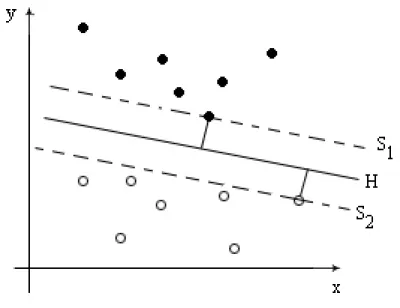
Figure 4.1: An example of a maximum-margin function H separating a training set.

the theory can be extended to n-dimensions and m-classifications. Assume we are given a set of training points {xk, yk}k=1n where x ∈ Rp and y ∈ {−1,1}. Our goal is to find a linear function H that divides the points in such a way that the line is as far away as possible from the closest sample in each set. We call these sample points support vectors. Since H is a linear function we can write it as

H(x) =hw,xi+b (4.4)

where w is a vector of weights and b is some offset. In order to maximize the margin between the function H and the closest sample points in each set we must find w and b. Figure 4.1 shows an example of the function H that we seek. Since we are trying to maximize the margin between H and the support vectors we can define the support functions S1 and S2 as

S1 =hw,xi+b= 1 (4.5)

S2 =hw,xi+b=−1. (4.6) Now we want to maximize the distance betweenS1 andS2. Applying simple geometry we can see that the distance between these two functions, or

hyper-planes, is also the distance where the hyperplane intersects the line through the origin and parallel to w. Let x+ _{correspond to the point on Equation} (4.5) and x− correspond to the point on Equation (4.6). Then

x+ = 1

||w||2w (4.7)

x− = −1

||w||2w, (4.8)

and the distance is

d(x+,x−) =||x+−x−||= 2

||w||. (4.9)

To maximize the distance in Equation (4.9) we need to minimize||w||. How-ever, we need to minimize||w||while ensuring our training data is appropri-ately classified. This results in the following optimization problem [25]

min||w|| subject to yi(hw,xii+b)≥1 ∀i, (4.10) which can be rewritten in terms of Lagrange multipliers as

L(w, b, α) = 1 2hw,wi − n X i=1 αi(yi(hw,xii+b)−1). (4.11) This optimization problem is well known and can be solved using standard quadratic programming techniques [25].

The maximal margin classifier is a good foundation for SVM theory, but since it requires the data to be linearly separable, it is not practical in real-world applications. A slack variable η was introduced into the optimization problem to calculate the hyperplane that would separate the data as cleanly as possible. As a result, the optimization problem in Equation (4.10) be-comes [25] min||w+C n X i=1 ηi|| subject to yi(hw,xii+b)≥1−ηi ∀i. (4.12)

4.3

Kernel Trick

Recall that the goal of the SVM is to find a linear function H that satisfies Equation (4.4) and separates the data as best as possible. The function is obtained by minimizing ||w|| with some constraint. Because H is a linear function, the weight vector will always be a linear combination of the training samples [25] w= N X i=1 αiyixi. (4.13)

Plugging this back into Equation (4.4) we get

H(x) = N

X

i=1

αiyihxi,xi+b. (4.14) Note the SVM operates in an inner product space. Recall from Chapter 2 that we can represent inner product spaces using a kernel function. With this in mind, we can reformulate the problem.

Letφ:X → H be some kind of mapping from the input space X to some feature space H. Let us assume the mapping takes the data in X which is not linearly separable, and makes it linearly separable inH. Let us apply the SVM method to this feature spaceH. Then we are looking for some function

H such that

H(x) =hw, φ(x)i+b. (4.15) But by Equation (4.13) we know w is a linear combination of the training samples so H(x) = N X i=1 αiyihφ(xi), φ(x)i+b. (4.16) Applying the kernel trick we see that

H(x) = N

X

i=1

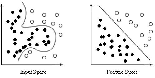
αiyiκ(xi,x) +b. (4.17) Let us examine what just happened. The feature spaceX contains data that is not linearly separable (Figure 4.2). However, using a kernel function, we are able to use some mapping φ to simultaneously represent our data in a linearly separable feature space. Applying the SVM in this feature space is

Figure 4.2: Example of the input space mapped to some feature space via a kernel function.

identical to applying some non-linear fitting model to our input space.

4.4

Evaluating Kernels Using Information Theory

The kernel method allows us to create non-linear classifiers. Of course, this is assuming the kernel is able to map the input space to a feature space where our data is linearly separable. Determining how well the data is linearized in the feature space requires us either to calculate the mappingφ, or to compute and test the classifier. Both of these options have significant drawbacks. In some cases it is not possible to calculate the mapping. For example, consider the Gaussian kernel case. If we apply Mercer’s theorem we see that the inner product space is infinite-dimensional. In other cases, computing or testing the classifier is too time consuming. We propose a method for evaluating how well a kernel linearizes a feature space by exploiting information theoretic measurements of the training data.

Recall what happens in the feature space when we estimate the R´enyi entropy and the Cauchy-Schwarz divergence from Chapter 3. In the inner product space produced by the kernel function, the estimator for R´enyi

en-tropy is just the squared norm of the mean of the transformed data Ip(X) = 1 N2 N X i=1 N X j=1 κ(xi, xj) (4.18) = 1 N2 N X i=1 N X j=1 hφ(xi), φ(xj)iH (4.19) = * 1 N N X j=1 φ(xi), 1 N N X j=1 φ(xJ) + H (4.20) =|| 1 N N X j=1 φ(xi)||2H (4.21) =||m||2 H. (4.22)

The estimator for CS divergence is the angle between the mean vectors of the two transformed data classes

ICS(p, q) =

hm,ni

p

hm,mihn,ni = cos∠(m,n). (4.23) If we use these estimates on the training data, we can characterize how well the classes are separated in the feature space.

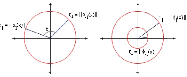
Let us assume {xk, yk}nk=1 wherex∈R2 and yk ∈ {−1,1}. If we calculate the Quadratic R´enyi entropy for each class by applying the estimator from Equation (2.34) then we will get the magnitude of the mean vector in the feature space. Letr1 =||φ1(x)||andr2 =||φ−1(x)||represent the magnitudes for each class. Since x ∈ _R2 _{we know the mean of each class must lie on a} circle of radius r1 and r2. If the mean values are close, or if r1 =r2, then all we know is that the mean of both our feature vectors lies on the radius of the same circle. But, if we use the CS divergence measure to calculate the angle between the two classes, we can figure out if the mean feature vectors have any separation on that circle. If the mean feature vectors vary enough, i.e. if r1 >> r2, then it is possible to assume the classes are separated well enough in the feature space without having to calculate the angle between them. Estimating these information theoretic measures using the input data allows us to evaluate how well the kernel function separates the data without having to explicitly compute the mapping or build the classifier.

Figure 4.3: Using the R´enyi entropy and CS divergence measures it is possible to classify how separated the classes are in the feature space.

CHAPTER 5

CONCLUSION

In most cases, the only way of evaluating how well a kernel operates in a support vector machine on a given set of input data is to build the classifier and test it on real data. This can take a long time depending on the size of the training set and the amount of available computational power. This thesis proposed a method for evaluating how well a kernel will separate classification classes in some feature space using information theoretic measure estimates on the input data. Even though the proposed method uses estimators that operate on the order of O(N2_{), this operation can be much quicker than} the standard quadratic optimization technique used in the SVM classifier. Furthermore, the proposed method implies that it may be possible to build an adaptive SVM that can evaluate how well the kernel is performing and make adjustments if necessary.

This thesis focused on information theoretic measures and how they could explain the kernel operations. Future research could be dedicated to finding new estimators that provide other important metrics in the feature space, for example, an estimator for the distance between two vectors. The proposed estimators are also primarily concerned with the mean values of the data in the feature space. This raises the question of whether or not it is possible to create estimators that can classify the variance of the data in the feature space.

REFERENCES

[1] K. Fukunaga, Introduction to Statistical Pattern Recognition, 2nd ed. San Diego, CA: Academic Press, Oct. 1990.

[2] R. O. Duda, P. E. Hart, and D. G. Stork,Pattern Classification, 2nd ed. New York, NY: Wiley-Interscience, Nov. 2001.

[3] C. E. Shannon and W. Weaver, The Mathematical Theory of Commu-nication. University of Illinois Press, Urbana, 1949.

[4] T. M. Cover and J. A. Thomas,Elements of Information Theory. Hobo-ken, NJ: Wiley-Interscience, 2006.

[5] R. V. L. Hartley, “Transmission of information,”Bell Syst. Tech. Jour-nal, vol. 7, pp. 535–563, 1928.

[6] A. R´enyi, “On measures of entropy and information,” in Proceedings of the 4th Berkeley Symposium on Mathematics, Statistics and Probability, 1960, pp. 547–561.

[7] J. Aczl and Z. Darczy, On Measures of Information and Their Char-acterizations. New York: Academic Press [Harcourt Brace Jovanovich Publishers], 1975.

[8] A. Renyi and P. Turan, Selected papers of Alfred Renyi. Budapest: Akademiai Kiado, 1976.

[9] C. Tsallis, “Possible generalization of Boltzmann-Gibbs statistics,” J. Statist. Phys., vol. 52, no. 1-2, pp. 479–487, 1988.

[10] E. Parzen, “On estimation of a probability density function and mode,”

The Annals of Mathematical Statistics, vol. 33, no. 3, pp. 1065–1076, 1962.

[11] J. Principe and D. Xu, “Information-theoretic learning using Renyi’s quadratic entropy,” inProc. 1st International Workshop on Independent Component Analysis and Signal Separation, Jan. 1999, pp. 407–412.

[12] E. Lutwak, D. Yang, and G. Zhang, “Cramerrao and moment-entropy in-equalities for Renyi entropy and generalized Fisher information,” IEEE Transactions on Information Theory, vol. 51, no. 2, pp. 473–478, 2005. [13] N. Aronszajn, “Theory of reproducing kernels,” Transactions of the

American Mathematical Society, vol. 68, pp. 337–404, 1950.

[14] L. M´at´e,Hilbert Space Methods in Science and Engineering. Budapest, Akademiai Kiado: A. Hilger, 1989.

[15] A. Berlinet and C. Thomas-Agnan, Reproducing Kernel Hilbert Spaces in Probability and Statistics. Norwell, MA: Kluwer Academic, 2004. [16] J. Mercer, “Functions of positive and negative type and their connection

with the theory of integral equations,” Philos. Trans. Royal Soc. (A), vol. 83, no. 559, pp. 69–70, Nov. 1909.

[17] A. Aizerman, E. M. Braverman, and L. I. Rozoner, “Theoretical founda-tions of the potential function method in pattern recognition learning,”

Automation and Remote Control, vol. 25, pp. 821–837, 1964.

[18] B. Sch¨olkopf, A. Smola, and K.-R. M¨uller, “Nonlinear component anal-ysis as a kernel eigenvalue problem,” Neural Comput., vol. 10, no. 5, pp. 1299–1319, July 1998.

[19] J. Shawe-Taylor and N. Cristianini, Kernel Methods for Pattern Analy-sis. New York, NY: Cambridge University Press, 2004.

[20] M. Girolami, “Orthogonal series density estimation and the kernel eigen-value problem,”Neural Comput., vol. 14, no. 3, pp. 669–688, Mar. 2002. [21] C. Cortes and V. Vapnik, “Support-vector networks,” Machine Learning, vol. 20, no. 3, pp. 273–297, Sep. 1995. [Online]. Available: http://dx.doi.org/10.1007/BF00994018

[22] V. N. Vapnik and Ya, “On the uniform convergence of relative frequencies of events to their probabilities,” Theory of Probability and its Applications, vol. 16, no. 2, pp. 264–280, 1971. [Online]. Available: http://link.aip.org/link/?TPR/16/264/1

[23] V. N. Vapnik, The Nature of Statistical Learning Theory. New York, NY: Springer-Verlag, New York, Inc., 1995.

[24] V. N. Vapnik, Statistical Learning Theory. New York, NY: Wiley, Sep. 1998.

[25] N. Cristianini and J. Shawe-Taylor, An Introduction to Support Vector Machines. New York, NY: Cambridge University Press, 2000.