Bayesian analysis of default and credit migration : latent factor models for event count and time-to-event data

(1)

Heriot-Watt University

Bayesian Analysis of Default and Credit

Migration: Latent Factor Models for

Event Count and Time-to-Event Data

Yongqiang Bu

June 25, 2014

Submitted for the degree of

Doctor of Philosophy in Mathematical Statistics on completion of research in the

Department of Actuarial Mathematics and Statistics, School of Mathematical and Computing Sciences.

The copyright in this thesis is owned by the author. Any quotation from the thesis or use of any of the information contained in it must acknowledge this thesis as the source of the quotation or information.

(2)

I hereby declare that the work presented in this the-sis was carried out by myself at Heriot-Watt University, Edinburgh, except where due acknowledgement is made, and has not been submitted for any other degree.

(Candidate)

(Supervisor)

(3)

Abstract

This thesis develops Bayesian models to explain credit default and migration risk. Credit risk models used in practice are based on an assumption of conditionally inde-pendent events given a realization of systematic risk factors. The systematic risk can be modelled with both observed and unobserved factors.

On the one hand we consider generalised linear mixed models (GLMMs) for default count data where random effects account for unobserved factor risk. On the other hand we consider survival models with shared frailties to model unobserved factors in time-to-default and time-to-rating-transition data. The latter models are developed in the Anderson-Gill counting process framework for the Cox proportional hazards model to allow multiple events and time-dependent covariates.

Using Standard and Poor’s data on default and rating transitions we control for observed macroeconomic factors in the fixed effect parts of the models. We allow the latent factors to have autoregressive time series structure.

The results from both kinds of model show clear evidence of heterogeneity between industry sectors/countries and time period suggesting that different latent factor ef-fects are present in different sectors. This is an important message that should be accounted for in risk analyses.

We implement Bayesian inference for all our models and use the MCMC approach (Gibbs sampling). We show some tractable model formulations that capture the main sources and implement Bayesian model choice procedures to select the most explanatory models.

(4)

There are couple of contributions in this thesis: First, this is an analysis of industry effects on default and migration rates using vector-valued random effects in default count models and vector-valued dynamic frailties in time-to-event/survival models. While this has been done before in models for default counts (McNeil-Wendin) it is quite novel for time-to-event models. Koopman, Lucas and Schwaab (2012) which has some similarities but the estimation is by Monte Carlo maximum likelihood, not by Bayesian methods. Second, estimation of rating transition model with shared dynamic frailties for different industry sectors and macroeconomic covariates using Bayesian techniques (MCMC). This is a new model which is based on a simpler model used in medical statistics (Manda & Mayer(2005)) that has been adapted and extended for the credit risk application. We show how to estimate the new model using a Bayesian approach. Finally, we use the model to compute point-in-time dynamic estimates of rating transition probabilities for different industry sectors and forecast these into the future, while taking into account macroeconomic factors. This can be very useful for risk management applications and economic scenario generation.

(5)

Acknowledgements

First and foremost, I would like to thank my supervisor, Prof. Alexander McNeil, for introducing me to the world of credit risk modelling, and for all advice and support that I have received during these years. Apart from the always pleasantly informal atmosphere of our research sessions, I especially appreciated his generosity with his time.

I would also like to thank Dr George Streftaris for his comments and advice on Win-Bugs. I am grateful to Prof. Andrew Cairns provide valuable and incomparable comments on my thesis. Thanks also due to all colleagues at Heriot Watt University who made my life at Edinburgh colorful.

Last, but not least, I would like to thank my family for their support and encourage-ment. Especially to my wife Mingxia and our children.

(6)

List of Tables

1.1 Numbers of transitions for Standard & Poors’ CreditPro 6.6 from 31/12/1980

- 31/12/2003 . . . 12

2.1 Numbers of industry sectors observations . . . 32

2.2 Model 2.1: GLMMs with equicorrelation structure fitted to 23 years historical Standard & Poor’s data . . . 33

2.3 Model 2.2: GLMM with different macroeconomic covariates . . . 36

2.4 Model 2.2 with macroeconomic covariate CFNAIMA3 spretl and GDP 42 2.5 Model 2.2 with macroeconomic covariate CFNAIMA3 and spretl . . . 42

2.6 Model 2.3 with industry sectors random effects . . . 42

2.7 Model 2.1: GLMMs with Equicorrelation structure . . . 44

2.8 Model with sector random effects and without sector random effects . 44 2.9 Model 2.4 with industry sectors random effects and CFNAIMA3 . . . 44

2.10 LogLik,AIC and BIC for four different models . . . 47

3.1 Numbers of obligors used for different industry sectors . . . 62

3.2 Model 3.1 with macroeconomic variable only . . . 63

3.3 Model 3.2 with yearly shared frailty . . . 65

(10)

3.5 Model 3.4: Model with shared sector frailties (have been omitted for a

simpler presentation) . . . 70

3.6 Deviance information criterion for four different Models . . . 73

4.1 Industry sectors used in our analysis . . . 84

4.2 Numbers of notches for Standard & Poors’ CreditPro 6.6 from 31/12/1980 - 31/12/2003 . . . 87

4.3 Model 4A.1 with macroeconomic variable only . . . 87

4.4 Model 4A.2 with yearly time-dependent shared frailty . . . 89

4.5 Model 4A.3 with serial dependence for yearly shared frailty . . . 91

4.6 Model 4A.4: Model with shared sector frailties (results have been omit-ted for a simpler presentation) . . . 93

4.7 Deviance information criterion for four different frailty models . . . . 94

4.8 Numbers of transitions for Standard & Poors’ CreditPro 6.6 from 31/12/1980 - 31/12/2003 . . . 99

4.9 Model 4B.1 with macroeconomic variable . . . 101

4.10 Model 4B.2 with yearly shared frailties . . . 104

4.11 Model 4B.2 with yearly shared frailties . . . 105

4.12 Model 4B.3 with serial dependence for yearly shared frailties . . . 108

4.13 Model 4B.3 with serial dependence for yearly shared frailties . . . 109

4.14 Model 4B.4 with shared sector frailties . . . 112

4.15 Model 4B.4 with shared sector frailties . . . 114

4.16 Deviance information criterion for four different frailty models . . . . 115

5.1 The one month transition matrix calculated using the homogeneous hazard rate methods. The matrix was calculated for the period from Jan1980 to Dec2003 . . . 120

(11)

5.2 The one month transition matrix calculated using the inhomogeneous methods for Dec2003 . . . 122

(12)

List of Figures

2.1 Empirical 6-month default rates for 23 years . . . 30

2.2 Historical macroeconomic covariates CFNAI, CFNAIMA3, SP500 re-turn and SP500 volatility . . . 34

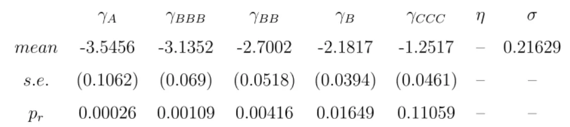
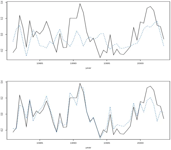
2.3 Visual comparison of systematic risk factors. The upper plot displays the estimated unobserved effect of factor {(t,Ψt) : t = 1, . . . , T} in

Model 2.1 (solid black line) and the estimated fixed factor CFNAI {(t, ztη) :t = 1, . . . , T}(dashed blue line) in Model 2.2. The lower plot

compare the unobserved factor for Model 2.1 (solid black line) and Model 2.2 with macroeconomic covariates CFNAI (dashed blue line). 38

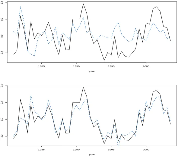
2.4 Visual comparison of systematic risk factors. The upper plot dis-plays the unobserved factor {(t,Ψt) : t = 1, . . . , T} of Model I

(sol-id black line) and observed fixed factor CFNAIMA3 {(t, ztη) : t =

1, . . . , T}(dashed blue line) in Model 2.2. The lower plot compare the unobserved factor for Model I (solid black line) and Model 2.2 with macroeconomic covariates CFNAIMA3(dashed blue line). . . 39

2.5 Visual comparison of systematic risk factors. The upper plot displays the unobserved factor {(t,Ψt) :t= 1, . . . , T} of Model 2.1 (solid black

line) and observed fixed factor Spretl {(t, ztη) : t = 1, . . . , T}(dashed

blue line) in Model 2.2. The lower plot compare the unobserved factor for Model 2.1 (solid black line) and Model 2.2 with macroeconomic covariates spretl(dashed blue line). . . 40

(13)

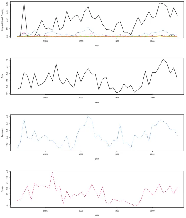
2.6 The top figure shows empirical default probability with different rating categories, the following three plots show {(t, bt) : t = 1, . . . , T} for

different industry Aero, Consumer and Energy random effects with rating category “CCC” . . . 45

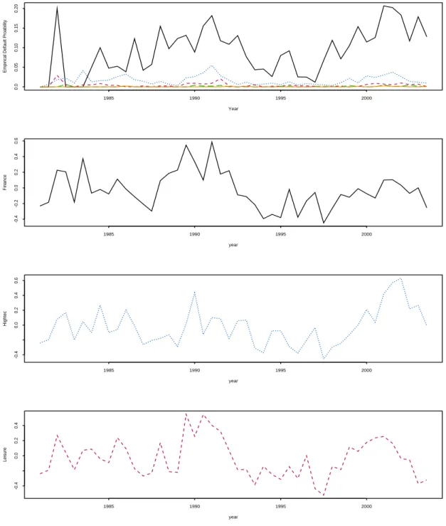
2.7 The top figure shows empirical default probability with different rating categories, the following three plots show {(t, bt) : t = 1, . . . , T} for

different industry Finance, Hightec and Leisure random effects with rating category “CCC” . . . 46

3.1 Intensity vs macroeconomic covariates in upper figure and monthly intensity for all five different rating categories with Model 3.1 . . . . 64

3.2 Monthly intensity for rating category BBB with Model 3.1; posterior means with 95% credible intervals . . . 64

3.3 Default intensity for rating category B: The blue plot displays the in-tensity for Model 3.1 with macroeconomic only and the red plot display the intensity with unobserved yearly shared frailty b in Model 3.2 . . 67 3.4 Monthly default intensity for rating categories B with Model 3.2;

pos-terior means with 95% credible intervals . . . 67

3.5 Default intensity for rating category BB. The black plot displays the default intensity for Model 3.1 with macroeconomic only and default intensity function with unobserved yearly frailty b in Model 3.2 (red line) and Model 3.3 (blue line) . . . 69

3.6 Monthly default intensity for rating categories BB with Model 3.3; posterior means with 95% credible intervals . . . 69

3.7 Different sector’s default intensity for rating category CCC . . . 71

3.8 Monthly default intensity for rating categories CCC with Model 3.4; posterior means with 95% credible intervals . . . 72

(14)

4.1 Monthly intensity for two notch downgrade VS two notch upgrade, the blue line shows downgrade and red line for upgrade . . . 88 4.2 Monthly intensity for two notches downgrade and upgrade; posterior

means with 95% credible intervals, the upper plot shows downgrade and lower plot for upgrade . . . 88

4.3 Monthly intensity for one notch downgrade and upgrade; posterior means with 95% credible intervals, the upper plot shows downgrade and lower plot for upgrade . . . 90 4.4 Monthly intensity for one notch downgrade for Model 4A.1 (red line)

and Model 4A.2 (blue line) . . . 90

4.5 Monthly intensity for one notch downgrade and upgrade; posterior means with 95% credible intervals, the upper plot shows downgrade and lower plot for upgrade . . . 92 4.6 Monthly intensity for one notch downgrade for Model 4A.1 (red line),

Model 4A.2 (black line) and Model 4A.3 (blue line) . . . 92 4.7 Monthly intensity for one notch downgrade with Model 4A.1 (black

line), Model 4A.4 (red and blue line) for different sectors . . . 95 4.8 Monthly intensity for one notch downgrade; posterior means with 95%

credible intervals, the upper plot shows sector Finance and lower plot for sector Forest . . . 96

4.9 Monthly intensity for downgrade and upgrade for rating BBB, the blue line shows downgrade and red line for upgrade . . . 102

4.10 Monthly intensity for transition BBB to BB; posterior means with 95% credible intervals . . . 102

4.11 Monthly intensity for rating transition AA to A, the blue line shows Model 4B.2 and red line for Model 4B.1 . . . 103

4.12 Monthly intensity for transition AA to A; posterior means with 95% credible intervals . . . 106

(15)

4.13 Macroeconomic covariates vs yearly shared frailty . . . 106

4.14 Monthly intensity for rating transition CCC to D, the blue line shows Model 4B.3, red line for Model 4B.2 and black for Model 4B.1 . . . . 107

4.15 Monthly intensity for transition CCC to D; posterior means with 95% credible intervals . . . 110

4.16 Macroeconomic covairates vs yearly shared frailty . . . 110

4.17 Monthly intensity for rating transition BB to B with Model 4B.1 (black line), Model 4B.4 (red and blue line) . . . 113

4.18 Monthly intensity for rating transition BB to B; posterior means with 95% credible intervals, the upper plot shows sector Energy and lower plot for sector Hightec . . . 114

5.1 Monthly transition probabilities for three different rating transitions . 123

(16)

Chapter 1 Introduction

Credit risk is the risk of the change in value of a portfolio caused by unexpected changes in the credit quality of borrowers, bond issuers or trading partners. Credit risk, together with market risk and operational risk, are the three fundamental risk categories in the banking sector of the financial industry.

The Basel Capital Accord requires banks to hold risk-weighted assets against future potential losses in order to manage the credit risk of business activities. Banks may choose between standardized and advanced approaches for measuring credit risk. In the advanced approach, banks are allowed to build their own internal-ratings-based (IRB) models for measuring certain aspects of credit risk. The IRB approach uses statistical techniques to estimate such quantities as probability of default (PD), loss given default (LGD) and exposure at default (EAD). This has stimulated the devel-opment of statistical models in credit risk. Furthermore, the Accord also requires financial institutions to establish rigorous procedures for the validation of statistical models. Thus the measurement and management of credit risk is of interest to both banks and regulators.

Banks need to estimate the credit rating transition probabilities (including default probability) and keep the probability estimation updated for risk management and e-conomic capital purpose. Banks need to compare realized transition probabilities with

(17)

the estimated probabilities to demonstrate models work reasonably. Those compar-isons must use historical data over a long time period. Probabilities of default (PDs) play a prominent role in the areas of pricing credit derivatives, portfolio management and capital allocation. They also determine banks’ regulatory capital requirements. For many years, a number of model solutions have been very successful in the financial industry, such as CreditMetrics (CreditManager by RiskMetrics, originally owned by JP Morgan), Portfolio Manager (Moody’s KMV), CreditRisk+ _{(Credit Suisse}

Finan-cial Products) and CreditPortfolioView (McKinsey). See Crouhy et al. (2000) for a survey. Since the whole industry still has relatively limited historical default data, these credit risk models do not rely on the formal statistical estimation for all param-eters from historical default data. Normally we separate the default probability and the parameters which describe the default dependence.

It is well understood that default probabilities partly depend on the macroeconomic situation and rating transitions are also influenced by macroeconomic variables. In building models it is necessary to confirm that this is the case and to find the most explanatory variables. However macroeconomic variables can not fully explain his-torical patterns of defaults and rating transitions, there is also a need for unobserved (latent) factors in models (McNeil and Wendin (2007)).

All four industrial models above belong to the class of factor models for the approach to dependence (Frey and McNeil (2003)). Gordy (2000) shows these three models share some similarities and can be mapped to each other. While CreditRisk+ _belongs

to the class of so-called reduced-form models for default modelling, CreditMetrics and Portfolio Manager adopt a structured modelling approach. However these are really issues of presentation and the probabilistic structure of the models is similar. In this thesis, we will describe two different statistical methods for modelling credit risk. These are generalized linear mixed models (GLMMs) which relate quite closely to the industry models described above and survival models with frailty.

Using both factor and reduced-form models, we need to find the most explanato-ry macroeconomic variables. Several researchers have tried to estimate the rating

(18)

changes process by finding some relevant explanatory variables. Nickel, Perraudin, and Varotto (2000) estimate a multivariate probit model by working with individual Moodys rating histories. They underline the importance of position in the economic cycle, of individual industry and geographic origin of every underlying firm. Bangia, Diebold, and Shuermann (2002) build quarterly transition matrices with expansions and recessions economic condition. They conclude that the rating transition process can be considered as markovian after conditioning by the state of the economy.

The time-homogeneity property normally assumes that rating migrations are stable over time. However, the time-homogeneity and Markovian behavior assumption have been challenged by many academic studies on the presence of various non-Markovian behaviors such as industry heterogeneity, rating drift and time variations. Several empirical studies have found time-variation in default rates and confirmed that varia-tion could be explained by observed macroeconomic variables; see Nickell, Perraudin, and Varotto (2000), Bangia, Diebold, and Shuermann (2002), and Hu, Kiesel, and Perraudin (2002). The time-varying migration probabilities have become an inter-esting implications for credit risk modelling when Standard & Poor’s rate corporate bonds through the business cycle. Issuer-specific effects in credit risk analysis also become popular in academic research in recent years. McNeil and Wendin (2006) and Koopman, Lucas, and Monteiro (2006) account for issuer-specific effects through latent factors for the business cycle. There is industrial heterogeneity in rating mi-grations (including default). In this thesis, we will account for both business cycle and industry specific effects by random effects in GLMMs and dynamic frailties in survival models.

There are three contributions in this thesis: First, this is an analysis of industry effects on default and migration rates using vector-valued random effects in default count models and vector-valued dynamic frailties in time-to-event/survival models. While this has been done before in default count models (McNeil and Wendin (2007)), it is quite novel for time-to-event models. Koopman, Lucas and Schwaab (2012) which has some similarities but the estimation is by Monte Carlo maximum likelihood, not

(19)

by Bayesian methods.

Second, estimation of rating transition model with shared dynamic frailties for differ-ent industry sectors and macroeconomic covariates using Bayesian techniques (MCM-C). This is a new model which is based on a simpler model used in medical statistics (Manda & Mayer(2005)) that has been adapted and extended for the credit risk appli-cation. We show how to estimate the new model using a Bayesian approach. It is very difficult to calibrate the time-to-event model because of the sparsity of data which often leads to unrealistic transition probabilities. Therefore we calibrate the model using Bayesian methods based on Markov Chain Monte Carlo (MCMC) techniques. Bayesian methods improve estimation accuracy especially for low frequency events. Stefanescu, Tunaru, and Turnbull (2009), who also advocate Bayesian methodology for calibrating models for rating transition probabilities using historical data, assert “Model calibration for this type of application is difficult in a classical frequentist estimation framework, because the sparsity of data often leads to unrealistic transi-tion probabilities”. Kadam and Lenk (2008) adopt Bayesian estimatransi-tion techniques for Moody’s corporate bond default database and shows strong country and industry effects on the determination of rating migration behavior. Bayesian estimation also allows expert opinion to be taken into account through the use of subjective prior distributions for model parameters. Credit rating process involves a large amount of non-quantifiable subjective information which experienced credit risk practitioner-s often help to exprepractitioner-spractitioner-s their opinionpractitioner-s. In the capractitioner-se of low default portfoliopractitioner-s, expert even gain more weight, especially in industry. Bayesian inference makes it straight-forward to compute derived quantities, for example default correlations, the default and transition probabilities, therefore it is increasingly popular; see for instance Nick-ell, Perraudin, and Varotto (2000), Bangia, Diebold, and Shuermann (2002), Kadam and Lenk (2008) and Stefanescu, Tunaru, and Turnbull (2009). Our model has some attractive features and can be estimated using a standard software package (BUGS), albeit quite slowly. BUGS offers the Deviance Information Criterion (DIC) which developed by Spiegelhalter et al. (2003) to examine the predictive ability of a model.

(20)

It is based on a Bayesian measure of predictive power. The model with the smallest DIC value is estimated to give the best predictions for a data set of the same structure as the data actually observed. The DIC measure has the advantage that it does not require the models to be nested for the purpose of comparison.

Finally, we use the model to compute point-in-time dynamic estimates of rating tran-sition probabilities for different industry sectors and forecast these into the future, while taking into account macroeconomic factors. This can be very useful for risk management applications and economic scenario generation.

1.1 Credit risk modelling using GLMMs

Altman (1968) produces an analysis of bankruptcy prediction using Z-scores (a credit scoring technique) in his seminal work. This multiple discriminant analysis performs logistic regression using many different accounting ratios. It has become popular among practitioners and provides the basic idea for further regression analyses of default. Merton (1974) assesses the credit risk of a company by characterizing the company’s equity as a call option on its assets. He then uses put-call parity to price the value of a put and this is treated as an analogous representation of the firm’s credit risk. This model has the limitation that it can only be used for companies with publicly traded equity. For non-listed companies, it is difficult to get asset and liability information.

Credit scoring technique is widely used in banks for building internal rating system in recent years. Banks use probability of default to arrange rating categories. Each rating can be mapped to a probability of default and obligors can be arranged in rating categories using probability of default. The credit rating gives a brief summary of obligors’ financial situation, so many banks adopt an internal rating for their own lending management. Merton’s model assesses credit risk from asset-liability to model distance to default (DD). Both credit scoring technique and Merton’s model allow practitioners to model credit risk. However, not every bank needs to or has the

(21)

ability to adopt an internal rating system. Therefore third-party rating agencies, such as Moody’s, Standard & Poor’s and Fitch rating are needed in financial markets. These rating agencies assess the creditworthiness of major publicly listed companies. Servigny and Renault (2004) give a comprehensive discussion of fundamental issues about credit rating.

When considering a portfolio of loans or bonds, the key issue is to model the joint default probability. We must consider the dependence because defaults do not oc-cur independently; knowing the default probability only is far from enough. The dependence between default events has a crucial impact on the upper tail of a credit loss distribution. Default intensities vary over time but share common risk which we refer to as systematic risk. Nickell, Perraudin, and Varotto (2000) and Hu, Kiesel, and Perraudin (2002) find time-variation in default rates and confirmed that this time-variation could be explained by observed macroeconomic variables. However, observed variables as proxies for the systematic risk are challenged for the following reasons. First, it is difficult to find appropriate proxies and they usually do not en-tirely explain the variability in default rates. Second, there may also be a lag between the cycle of a proxy variable and default activity. The lag may vary stochastically over time. These shortcomings can be remedied by latent factors. Koopman, Lucas and Klaassen (2005) give further details about the advantages of latent risk factors. It allow us to capture time-inhomogeneity in default rates and heterogeneity across individual obligors, industry sectors, or any other desired groupings like country with a well-chosen fixed and random effects.

Analytical maximum likelihood techniques can be used for relatively simple models that do not incorporate serial dependence; see for Gordy and Heitfield (2002), Frey and McNeil (2003), and Rosch (2005). McNeil and Wendin (2007) adopt a computational Bayesian methodology with Gibbs sampling with serially correlated random effects. There are some literatures on fitting such models to default data. Crowder et al. (2005) consider a model for default counts with a two-state latent systematic factor following a Markov chain. Gagliardini and Gourieroux (2005), and Koopman, Lucas

(22)

and Klaassen (2005) consider models where default risk is driven by continuous latent factors using the ratio of defaulted obligors instead of the actual default counts.

Mixture models are also referred as factor models or conditional independence mod-els. Depending on a set of common economic factors like macroeconomic covariates or latent factors, defaults are assumed to be independent. We will start from the premise of conditionally independent default given a realization of relevant system-atic risk factors. The dependence of individual default probabilities comes from the common factors. We will focus on Bernoulli mixture models for our analysis; other mixture model like Poisson mixture model can be found in McNeil, Frey, and Em-brechts (2005). McNeil and Wendin (2007) highlight the usefulness of generalized linear mixed models (GLMMs) in the modelling of portfolio default risk. Both ob-served and unobob-served risk factors can be accommodated by the class of generalized linear mixed models (GLMMs). McNeil and Wendin (2007) and Stefanescu, Tunaru and Turnbull (2009) use Chicago Fed National Activities Index (CFANI) as an im-portant explanatory variable for US firms. There may be a lag between the cycle of macroeconomic variables and that of default activity, we include three months moving average of Chicago Fed National Activities Index (CFANIMA3) in our analysis. And we will compare different macroeconomic covariates in our first set of analyses and then use the best ones in subsequent.

Both McNeil and Wendin (2007) and Stefanescu, Tunaru and Turnbull (2009) use a Bayesian approach to fitting the model with Markov chain Monte Carlo (MCMC) techniques. However there are some nice existing standard software packages which can be used for GLMMs instead of using the complicated Bayesian and MCMC tech-niques. We use theglmefunction in the S-Pluscorrelated data libraryfor the following analysis. The R function glmmPQL is an alternative choice. However, the R func-tionglmmPQL can be treated as a special case of glmewith (RE)P QLmethod. In S-plus glmeis a more general function; there are four different methods that can be used in fitting models and these are “AGQUAS”,“LAPLACE”, (restricted) penalized quasi-likelihood ((RE)PQL) and (restricted) marginal quasi-likelihood ((RE)MQL)

(23)

method. However, (RE)PQL and (RE)MQL gives similar results. Methods AGQUAD and LAPLACE are restricted to family binomial(“logit”) or poisson(“log”). The “pro-bit” link function makes it straightforward to calculate default probability for our one factor model in this analysis, we choose to use the default methods which are “(RE)PQL”.

1.2 Credit risk modelling using survival analysis

In the first part of this thesis, we analyse event count data using GLMMs. However, we are not only interested in the number of companies that migrate from one rating category to another, but also interested in the time period the company spends in a certain rating category. Hence, we will study the time-to-event analysis which has become popular in credit risk modelling in recent years. Cox’s hazard model has been increasingly used to model the hazard of credit risk events these years. In his seminal work, Cox (1972) proposes the proportional hazards model, where it is possible to estimate the relative intensity of a decrement without specifying the baseline intensity. Cox (1975) demonstrates the estimation procedure for the proportional hazards model with partial likelihood estimation. Andersen and Gill (1982) generalize the model to allow time-varying covariates using a counting process formulation, and show that the maximum partial likelihood estimates are asymptotically equivalent to unconditional maximum likelihood estimates.

As in our count data analysis for GLMMs, we need to capture the time and indus-try sector heterogeneity using unobserved random variables in survival analysis. The random effects in GLMMs are named frailty in survival framework. Frailty in sur-vival models help to capture heterogeneity with unobserved random variables. We introduce a frailty-based survival model for modelling the intensity of credit rating transitions (default). This type of model is an extension of the Cox proportion-al hazards models where a common random variable is used to account for hetero-geneity. “Frailty models” in survival analysis could capture the unexplained part of

(24)

the traditional Cox proportional model which take the function of random effects in GLMMs. The frailty factor captures default clustering beyond what can be explained by observed macroeconomic variables and firm-specific information. The unobserved component can capture effects with time or industry sector which show default de-pendence. Default intensities vary over time and shows co-movements in common or correlated risk factors that all firms are exposed to. Contagion is direct business liaisons between obligors a company may itself face increased risk if one of its major customers defaults. Davis and Lo (2001), and Egloff, Leippold, and Vanini (2007) has investigated this phenomenon.

Kavvathas (2001) and Couderc and Renault (2005) use a similar duration approach conditional on observed macro-variables and they show that average time-to-default decreases as economic activity decreases. Shumway (2001) develops a more dynamic bankruptcy prediction model by combining both financial ratios and market-driven measures and argues that discrete-time is necessary to calibrate hazards because of the intermittency of accounts information. Chava and Jarrow (2004) extend Shumway’s (2001) analysis to consider industry sector heterogeneity using monthly intervals. Duffie, Saita, and Wang (2007) formulate a doubly stochastic model for firm survival using firm-specific and macroeconomic covariates.

A credit rating summarises the credit worthiness of an individual, corporation, or even a country. It is an evaluation made by credit bureaus of a borrower’s overall credit history. A credit rating is also known as an evaluation of a potential borrower’s ability to repay debt, prepared by a credit bureau at the request of the lender. Credit ratings are calculated from financial history and current assets and liabilities. Typically, a credit rating tells a lender or investor the probability of the subject being able to pay back a loan and its interest.

We adapt a simpler model used in medical statistics (Manda and Mayer(2005)) and extended for the credit risk application. We estimate rating transition model with shared dynamic frailties for different industry sectors and macroeconomic covariates using Bayesian techniques (MCMC). This is a model that each transition intensity

(25)

follows a Cox type multiplicative regression model with frailties, two level frailties to account for both time period and industry sector heterogeneity. Delloye, Fermanian and Sbai (2006) define a reduced-form credit portfolio model which treat rating transi-tion as independent competing risks with conditransi-tionally independent and proportransi-tional hazards assumption. They also allow strong dependence levels by adding heterogene-ity. However, Delloye, Fermanian and Sbai (2006) split the Standard & Poors’ data into several groups based on the similar rating transition type and analyze these sep-arately. We consider the whole transition data and let all rating transitions share the same macroeconomic covariates and unobservable random process for all companies in monthly interval.

We consider credit survival model for both default and transition risk and there are two kinds of model were implemented for transition risk. The first one is frailty model for credit rating transitions by numbers of levels (notches) which is a simpler case for credit migration data. It is easy to handle but sacrifice the accuracy for rating transition, therefore we finally model the actual rating transitions. We have shown heterogeneity of transition risk over time and industry sector. We can also show heterogeneity for different countries if we extend our database to all the countries in Creditpro database. For estimation of these models, there are several ways to implement Gibbs simulation. WinBUGS is one of the most popular ways to implement Gibbs simulation. We use the model to compute point-in-time dynamic estimates of rating transition probabilities for different industry sectors and forecast these into the future, while taking into account macroeconomic factors. This is very useful for risk management applications and economic scenario generation.

1.3 Data description

The Standard & Poor’s database CreditPro 6.6 which consists of 10439 companies from 13 industry sectors over the period January 1981 to December 2003, 6897 of

(26)

them are US obligors. The rating classes included in the database are

K={CCC, B, BB, BBB, A, AA, AAA, D}

where we merge actual rating k+_{, k, k}− _into _k_{. We also merge} _{CCC, CC,} _and _C _into

a single rating class CCC. Rating class AAA and AA which rarely default have been excluded from the default study but be reconsidered in our transition analysis. More than 75% of the companies in the database from US and it is difficult to find macroeconomic covariates to explain credit quality changes for all different countries obligors. The study in this thesis has been restricted to US obligors.

In GLMMs, the default count data have been collected for semester-based periods rating from January 1981 to December 2003 giving a total of T = 46 periods. The yearly-based period miss many default events because many obligors migrate many times within one year, therefore we will misreport the default rating, while quarterly data improves the accuracy but too few default events in quarterly period. After comparing these three different data structure, we choose semester-based period in this default study with GLMMs.

In the time-to-event analysis, we choose one month as the time unit. Firstly our macroeconomic covariates are recorded in monthly which match the monthly unit. Secondly, monthly data record most of the transition activities, only very few have transition within one month, the daily would be ideal but it cannot be handled by WinBUGS. Although we use monthly time unit for data manipulation, the time shared frailty is yearly. There are overall 19054 effective rating migrations are recorded in the CreditPro database as well as 1386 defaults. Among them, 13526 effective rating migration as well as 1121 defaults are from US obligors. In time-to-event analysis, we assume the rating migrations only depend on macroeconomic covairates, time period and industry. Without any firm-specific covariates, we only interest in rating migration regardless the obligors. 1.1 shows all the possible transitions in our analysis. We studied default case only in chapter 3 and migration case in chapter 4 with two different models.

(27)

AAA AA A BBB BB B CCC D Total AAA 206 148 14 2 2 0 0 0 372 AA 44 481 553 34 5 5 1 0 1123 A 11 285 1246 840 57 27 1 5 2472 BBB 5 27 521 1342 659 72 9 19 2654 BB 3 8 46 483 1147 883 53 64 2687 B 1 7 25 48 520 1382 850 354 3187 CCC 1 0 4 7 18 129 193 679 1031 Total 271 956 2409 2756 2408 2498 1107 1121 13526

Table 1.1: Numbers of transitions for Standard & Poors’ CreditPro 6.6 from 31/12/1980 - 31/12/2003

1.4 Outline of the thesis and main contribution

In this thesis, we model credit risk using two different statistical models which are GLMMs and survival models with frailties. The thesis is structured as follows:

In Chapter 2, we model credit risk using GLMMs and consider the default risk only in this chapter. The Standard & Poor’s default count data is used for modelling in this chapter. We allow two levels of heterogeneity for both different times and industries which are represented by random effects in GLMMs framework. We also find three month moving average of Chicago Fed National Activities Index (CFNAIMA3) is the best observed macroeconomic variable to describe the credit default among the macroeconomic variables for US market. We find evidence of significant differences between industry sectors. In Chapter 3, we model default risk using survival model with frailties. We extend the Manda and Meyer (2005) model to allow two levels of random effects and apply this to credit risk modelling for the first time. The Standard & Poor’s default time-to-event data is used for modelling in this chapter. We allow two levels of heterogeneity for both different times and industries using survival frailties and serially correlated latent factors. Bayesian inference with Gibbs

(28)

sampler and WinBugs is used in this chapter. In Chapter 4, we extend the model for default risk to allow multiple events which are ratings transitions. In Chapter 5, we use the intensities results to calculate the credit rating transition probability matrices and give an conclusion in Chapter 6.

(29)

Chapter 2 Modelling default risk with

GLMMs

Most credit risk models used in practice are based on an assumption of conditionally independent defaults given a realization of systematic risk factors, such models are often referred to as mixture models. The systematic risk can be modelled with both observed factors and unobserved factors. Statistical models from the class of general-ized linear mixed models (GLMMs) take observable and unobservable factors as fixed effects and random effects respectively. Generalized linear model (GLM) is a special case of the GLMM which has no random effects. The random effects in GLMMs help to capture patterns of variability in the response that cannot be explained by the observable factors. The random effects may be scalar or vector. For example, in this thesis both time and industry sector are often treated as two different levels of random effect in default analyses.

There is general lack closed forms for latent factors yields joint default distribution in the form of integrals. Relatively simple models that do not incorporate serial de-pendence can use analytical maximum likelihood techniques examples include Gordy and Heitfield (2002), Frey and McNeil (2003), and Rosch (2005). McNeil and Wendin (2007) test several models with fixed and random effects using latent factor formu-lation by Bayesian techniques. Stefanescu, Tunaru and Turnbull (2009) develop a

(30)

credit rating process model to capture rating transition patterns and estimate it with Bayesian as well. Bayesian methods improve the estimation accuracy especially for low frenquency events. Bayesian estimation also allows expert opinion to be taken through the use of subjective prior distributions for model parameters. Credit rat-ing process involves a large amount of non-quantifiable subjective information which experienced credit risk practitioners often help to express their opinions. In the case of low default portfolios, expert even gain more weight. Bayesian inference becomes straightforward to compute the default and transition probabilities, therefore it is increasingly popular. However, these are a number of software packages for GLMMs based on ML-methodology. The advantage of these defined function is that they are simple and very easy to handle. These defined functions use maximum likelihood inference. We choose to use the glme function in the S-Plus correlated data library for the following analysis.

In this chapter, we will briefly introduce the mixture models, generalized linear mixed models and GLMMs first. Then we will express the mixture models as GLMMs. We will show how standard software can yield point-in-time(PIT) estimates of default probabilities and illustrate the method using Standard & Poor’s CreditPro data but we will provide comparative results with credit risk models using survival models which will be discussed in the next chapter. Alternatively, that may be one or more random effects included in this analyses, with the industry sector random effect, we will investigate differences in default probabilities between industry sectors.

2.1 Theory

2.1.1 One-period mixture models

Default risk is assumed to be driven by systematic risk factors, which might be ob-served macroeconomic covariates but might also be latent factors. Given a realization of these factors, defaults of individual firms are assumed to be independent. There are

(31)

several types of mixture models, such as Bernoulli mixture models and Poisson mix-ture models. More details about these mixmix-ture models can be found in McNeil, Frey and Embrechts (2005). Here we consider Bernoulli mixture models in this analysis.

Bernoulli distribution

Consider a portfolio of m obligors. Defaults in a fixed period can be modelled by multivariate Bernoulli distribution. Consider a fixed time period [0,T] and let τi be

the random time-to-default for obligor i, i∈ {1, . . . , m}. The default indicator Yi is a

Bernoulli random variable defined by Yi =I(τi ≤T) so that

P(Yi = 1) = 1−P(Yi = 0) =P(τi ≤T) =:P Di

where P Di is the default probability for obligor i.

Bernoulli mixture model

Give somep < mand a p-dimensional random vector Ψ= (Ψ1, . . . ,Ψp)0, the random

vector Y = (Y1, . . . , Ym)0 follows a Bernoulli mixture model with factor vector Ψ, if

there are functions pi :Rp →[0,1],1≤i≤m,such that conditional on Ψ the default

indicator Y is a vector of independent Bernoulli random variables with P(Yi = 1 |

Ψ=ψ) = pi(ψ). Fory= (y1, . . . , ym)0 in{0,1}m we have P(Y =y|Ψ=ψ) = m Y i=1 pi(ψ)yi(1−pi(ψ))1−yi

and the unconditional distribution of the default indicator vector Y is obtained by integrating over the distribution of the factor vector Ψ.

P(Y1 =y1, . . . , Yn=yn) = Z · · · Z Rp m Y i=1 pi(ψ)yi(1−pi(ψ))1−yidG(ψ)

(32)

Exchangeability and mixture models

To simply the analysis we will often assume that default indicator are exchangeable for obligors in a group. The sequence Y1, . . . , Ym of random variables is said to be

exchangeable if

(Y1, ..., Ym)

d

= (YΠ(1), . . . , YΠ(m))

for any permutation (Π(1), . . . ,Π(m)) of 1, . . . , m. For a group of similarly rated com-pany without any other information, the assumption of exchangeability is stronger than merely assuming identical marginal distribution of Y1, . . . , Ym but weaker than

assuming Y1, . . . , Ym to be independent and identically distributed (i.i.d). We

intro-duce a simple notation for default probabilities where

π:=P(Yi = 1), i∈ {1, . . . , m}

is the default probability of any obligor and

πk :=P(Yi1 = 1, . . . , Yik = 1), {i1, . . . , ik} ⊂ {1, . . . , m}, 2≤k≤m

is the joint default probability fork firms. When default indicators are exchangeable we get

E(Yi) =E(Yi2) = P(Yi = 1) =π, ∀i,

E(YiYj) = P(Yi = 1, Yj = 1) =π2, ∀i6=j,

so that cov(Yi, Yj) =π2−π2; then default correlation is give by

ρY :=ρ(Yi, Yj) =

π2−π2

π−π2 , ∀i6=j (2.1)

Exchangeable Bernoulli mixture models

Let m denote the number of observed companies and M denote the number that default. Assume that all the pi are identical function. Bernoulli mixture model is

exchangeable since default indicatorY is exchangeable. Let us introduceQ:=p1(Ψ)

(33)

of defaults M is the sum of m independent Bernoulli variables with parameter q. It is given by a binomial distribution with parameters q and m.

P(M =k |Q=q) = m k qk(1−q)m−k

The unconditional distribution of M is obtained by integrating over q

P(M =k) = Z 1 0 m k qk(1−q)m−kdG(q)

The default probability and joint default probabilities for the exchangeable group are given by:

π =E(Y1) =E(E(Y1 |Q)) =E(Q)

πk =P(Y1, . . . , Yk = 1) =E(E(Y1, . . . , Yk |Q)) =E(Qk)

Fori6=j

cov(Yi, Yj) = π2−π2 = var(Q)≥0,

The default correlationρY defined in (2.1) for exchangeable Bernoulli mixture model

is always non-negative.

Firm-valued models as Bernoulli mixture models

The Merton model is the prototype of all firm-value models. Merton model has been extended over the years but the original remains an influential benchmark and is still popular in credit risk analysis. A firm i whose asset value follows some stochastic process Vt,i has one single debt with face value Bi and maturity T. The process Vt,i

follows a diffusion model under real-world probability measure P

dVt,i =µVt,idt+σViVt,idWt

which implies that

VT ,i =V0,iexp (µVi− 1 2σ 2 Vi)T +σViWT ,i

(34)

The default probability of firm i is given by P(VT ,i ≤Bi) = P(lnVT,i ≤lnBi) = Φ ln Bi V0,i −(µVi − 1 2σ 2 Vi)T σVi √ T

Industry models can be re-written as mixture models. We assume that default occurs for obligor i if a critical value Xi (asset value, VT ,i in Merton’s model) lies below a

critical threshold di (liabilities, Bi in Merton’s model) at the end of each time

peri-od. KMV/CreditMetrics is industry credit risk models using Merton-type structure. They can be expressed by a mixture model. In order to apply these models at port-folio level require a multivariate Merton’s model. Assume that we have m companies and that the multivariate asset-value process (Vt) with Vt = (Vt,i, . . . , Vt,m)

0

follows anm-dimensional geometric Brownian motion with drift vectorµV = (µVi, . . . , µVm)

0 , vector of volatilities σV = (σVi, . . . , σVm)

0

and instantaneous correlation matrix P. This implies that for any firm i default occurs when some critical rv Xi :=XT,i lies

below some critical deterministic threshold di at the end of the time period [0, T].

In Merton’s model Xi is a log-normally distributed asset value and di represents

lia-bilities. Here we typically use multivariate log-normal or normal distribution for the vector X = (Xi, . . . , Xm)

0

. The dependence among defaults comes from the depen-dence among the components of the vector X.

We consider a portfolio of m obligors and fix a time horizon T. For 1 ≤ i ≤ m, we let rv Si be a state indicator for obligori at time T and assume that Si :=ST ,i takes

integer values in the set 0,1, . . . , nrepresenting rating class. We interpret 0 as default state. Here we will concentrate on the binary outcomes of default and non-default and ignore the finer categorization of non-defaulted companies. We writeYi :=YT,i for the

default indicator variable so thatYi = 1 ⇔Si >0. Random vectorY = (Yi, . . . , Ym)

0 is a vector of default indicators for the portfolio and p(y) = P(Y1 = y1, . . . Ym =

ym),y∈(0,1)m is its joint probability function; the marginal default probabilities are

denoted by ¯pi =P(Yi = 1), i= 1, . . . , m. The default correlations are defined to be the

(35)

then we obtain for firms i and j, withi6=j, ρ(Yi, Yj) = E(YiYj)−p¯ip¯j p ( ¯pi−p¯i2)( ¯pj −p¯j2) (2.2)

It is important to distinguish the default correlation ρ(Yi, Yi) of two firms i6=j from

the asset correlation which is the correlation of the critical variables Xi and Xj.

The vector of critical variables X is assumed to have a multivariate normal distri-bution and Xi can be interpreted as a change in asset value for firm i over the time

horizon of interest; di1 is chosen so that the probability that Xi ≤ di1 matches the

given default probability ¯pi for firm i.

The covariance of X is calibrated using a factor model. We assume that X can be written as

X =BF +ε (2.3)

for a p-dimensional random vector of common factors F ∼ Np(0,Ω) with p < m, a

loading matrix B ∈ _Rm×p_{, and an} _m_{-dimensional vector of independent univariate}

normally distributed errors ε, which are also independent of F. The factor structure (2.3) implies that the covariance matrix P of X (which will be a correlation matrix due to our assumptions on the marginal distribution ofX) is of the forP =BΩB0+Υ, where Υ is the diagonal covariance matrix of ε.

The conditional independence of defaults given Ψ follows from the independence of the idiosyncratic terms ε1, . . . , εm. Take bi = (bi1, . . . , bip)

0

for the ith row of B, the

ith critical variable has the following structure:

Xi =b0iF+εi (2.4)

where εi ∼N(0,1−βi) with βi = var(b0iF) =b

0

iΩbi , independent of Fand of εj for

j 6=i . Xi can represent lnVT in Merton’s model.

Asset correlation

The three most important drivers in determining portfolio credit risk are default probability(PD), loss given default (LGD) and default correlation. The most

(36)

com-mon approach to modelling default correlation (defined in equation 2.2)is to combine default probability with asset correlation. Therefore asset correlation is a critical driver in modelling portfolio credit risk. Two obligors will default in the same time if both of their asset value is smaller than their obligations. Asset correlation helps define the joint behavior of the asset value of two obligors. The asset correlations show how the asset value of one obligor depends on another obligor’s asset value. The correlation can also be described as the dependence of the asset value of an obligor on the general state of the economy and all obligors are depend on the state of economy which can be described by macroeconomic covariates.

Basel III IRB framework gives a formula for credit risk charge for an exposure using asset correlation ρ which is the average asset correlation of all pair-wise asset corre-lation in the portfolio. Here we consider the asset correcorre-lation using (2.4). The asset correlation between companies iand j is given by

ρ(Xi, Xj) = cov(Xi, Xj) = E(XiXj) = b0iΩbj

The asset correlation for practical models will be described in the models we use.

2.1.2 Generalized linear mixed models and its estimation

Clayton (1996) gives a very good overview of generalized linear mixed models(GLMMs). The special case of GLMMs without random effect all known as generalized linear models (GLMs). The random effects not only determine the correlation structure between observations on the same group, they also take account of heterogeneity a-mong groups that is attributed to unobserved factors. We will start with generalized linear models and then extend GLMs to GLMMs by adding random effects. Different inference methods for GLMMs will be introduced.

Generalized linear mixed models

Generalized linear models (GLMs) extend the linear model to allow distributions from the exponential family. The outcome of the response variables, Y = (y1, . . . , yn)0, is

(37)

assumed to be generated from a particular distribution function in the exponential family. The mean, µ≡(µ1, . . . , µn)0, of the distribution depends on the explanatory

variables, X ∈ Rn×p_{, through:}

E(Y) = µ=g−1(Xβ)

whereE(Y) is the expected value ofY,β= (β1,· · · , βp);Xβ is the linear predictor,

a linear combination of unknown parameters,β; g is the link function. The unknown but fixed regression parameters inβare estimated by solving the maximum likelihood equations. Generalized linear models (GLMs) consists of three components: A distri-bution functionf from the exponential family; a linear predictorη =Xβ; and a link functiong such thatE(Y) = µ=g−1(η). The link function provides the relationship between the linear predictor and the mean of the distribution function. There are many commonly used link functions, such as probit and logit link function in the Bernoulli case and log-link function in the Poisson case. Here we give the common response functions (g−1) for Bernoulli-type GLMMs.

• Probit Φ(x) = (1/p2π) Z x −∞ exp(−u2/2)du • logit ex/(1 +ex) = 1/(1 +e−x) • complementary log-log 1−exp(−ex)

Generalized linear mixed models (GLMMs) are GLMs with one or more random effects. The linear predictor should be rewritten as

η=Xβ+Zψ

where the fixed effectβ remains the same as in GLMs and random effects ψ are ran-dom variables drawn from a distribution. The ranran-dom effects generate heterogeneity

(38)

beyond that which can be captured with fixed effects. We firstly consider a single shared random effect in every time period in our model. Then we consider different random effects for different sectors. This will capture additional variability associated with economic effects in different sectors. X are fixed vector and could be rating and macroeconomic covariates in credit risk models,β are the corresponding fixed effects. While Z are random vectors and could be year and industry sectors, ψ are random effects.

Estimation of GLMMs

We can estimate the GLMMs parameters using Markov Chain Monte Carlo(MCMC) methods from a Bayesian point-of-view. Bayesian MCMC approach allows us to handle more complex models than standard packages. Furthermore, the Bayesian approach can work well for sparse default data. For a Bayesian approach to GLMMs of portfolio credit risk, see McNeil and Wendin (2007) for more information. However, some standard package like S-plus and R provide some defined functions for estimation of GLMMs. The advantage of these defined function is that they are simple and very easy to handle. These defined functions use maximum likelihood inference. We will give more details about maximum likelihood inference in the next paragraph.

Maximum likelihood (ML) inference for GLMMs is only really a possible option for the simplest model. The unconditional distribution is obtained by integrating the random effects. Factor models have conditional independence property, if we write

pYt,i|Ψt(y|ψ) for the conditional probability mass function of Yt,i given Ψt,

L(β, σ;data) = Z · · · Z n Y t=1 mt Y i=1 pYt,i|Ψt(Yt,i |ψ) f(ψ1, . . . , ψn)dψ1. . . dψn

wheref denotes the joint density of the random effects. With theiidGaussian random effects with marginal Gaussian densityfΨ, we can reduce then−dimensional integral

to L(β, σ;data) = n Y t=1 Z mt Y i=1 pYt,i|Ψt(Yt,i |ψ)fΨ(ψt)dψt

(39)

with the product of one-dimensional integrals. This can be easily solved the unknown parameters.

For those complicated models where the exact likelihood function is difficult to com-pute, approximation becomes unavoidable. There are several methods including pe-nalized quasi-likelihood (PQL), marginal quasi-likelihood(MQL), Laplace and adap-tive gaussian quadrature. More details about PQL and MQL can be found in Breslow and Clayton (1993).

We use the glme function in the S-Plus correlated data library for the following analysis. The R functionglmmPQLis an alternative choice. However, the R function

glmmPQL can be treated as a special case of glme with (RE)P QL method. In S-plus glme is a more general function; there are four different methods that can be used in fitting models and these are “AGQUAS”,“LAPLACE”, (restricted) penalized quasi-likelihood ((RE)PQL) and (restricted) marginal quasi-likelihood ((RE)MQL) method. However, (RE)PQL and (RE)MQL gives similar results. Methods AGQUAD and LAPLACE are restricted to family binomial(“logit”) or poisson(“log”). The “probit” link function makes it straightforward to calculate default probability for our one factor model in this analysis, we choose to use the default methods which are “(RE)PQL”.

2.1.3 Multi-period mixture models

Notation

Consider a multi-period model, we can write the general latent variable factor model as

Xit =b0itFt+it (2.5)

where Ft ∼ Np(0,Ω) and it ∼ N(0,1 − βit) with βit = var(b0itFt) = b0itΩbit.

F1,· · · , Ftdoes not necessary to bei.i.d. Xitcan represent lnVT in Merton’s model. In

(40)

so that the conditional default probability is given by P(Yit= 1 |Ft) = P(it ≤dit−b0itFt|Ft) = Φ dit √ 1−βit − b 0 itFt √ 1−βit (2.6)

and the unconditional default probability by pit= Φ(dit).

In this simple case of (2.5) where is only one factor we have

Xit =bitFt+

q

1−b2

itZit

for iid standard normal variablesFt, Z1t, Z2t, . . . and a common loading−1< bit <1.

The asset correlation between credit risks i and j in time period t is given by ρijt =

bitbjt and the conditional default probabilities by

P(Yit = 1|Ft) = Φ dit p 1−b2 it − _pbitFt 1−b2 it ! . (2.7) Mixture models as GLMMs

In one-period setting, we assume conditional default probabilities pi(Ψ) follows

pi(Ψ) =h(µ+β

0

xi+ Ψ)

where h is a link function, such as probit, logit and complementary log-log which are commonly used in GLMMs. The vector xi contains covariates for company i,

such as company specific information or industry, country group β and µ are model parameters. The random variable Ψ ∼ N(0, σ2_{) is normally distributed with scale}

parameter σ.

This model can be extended into multi-period model which is suitable for default counts for different time periods. Consider a series of mixing variables Ψ1, . . . ,Ψn

generate default dependence in each time period t = 1, . . . , n. The default indicator

Yt,i for company iin time periodtis assumed to be Bernoulli with default probability

pt,i(Ψt) depending on Ψt

pt,i(Ψt) =h(µ+x

0

t,iβ+ Ψt)

(41)

Dynamic latent effect

Both the one-period and multi-period Bernoulli mixture models belong to GLMMs family. The role of the random effects in GLMMs is to capture patterns of variability in the responses that cannot be explained by the observed covariates only. These non-observed factors could be time-period effect which we treat as the state-of-the-economy in that time period.

The GLMM framework allows more complexity by adding further random effects to obtain multi-factor mixture models. In our analysis, we also consider industry sector effects nested inside the time-period effects which is two-levels random effects. We can capture additional variability in different industry sectors in addition to the global variability given by time-period effect.

2.2 Models used in practice

It is useful to consider a one-factor model in many practical situations. The infor-mation may not always be available to calibrate a model with more factors, and one-factor models may be easily fitted statistically to default data. Here we consider the models for default risk with GLMMs.

2.2.1 Model 2.1: One-factor model with Equicorrelation

struc-ture

Let us consider the case where the default probability depends only on the credit ratingr(i, t) of theith individual in periodt and where loadingsbitfor all individuals

in all time periods are the same so that

P(Yit = 1|Ft) = Φ _Φ−1₍_p r(i,t)) √ 1−b2 − bFt √ 1−b2 ,

(42)

where b is the common loading and the asset correlation is ρ = b2_{. This model can}

be written in simpler GLMM notation as

P (Yit = 1|Ψt) = Φ γr(i,t)+ Ψt

where γr is a fixed rating effect and Ψt ∼ N(0, σ2) is a random effect for period t.

The parameters in the credit risk model and the GLMM are related by

ρ=b2 = σ 2 1 +σ2 pr = Φ γr √ 1 +σ2

so that both asset correlation and rating class default probabilities may be inferred from the fitted GLMM.

2.2.2 Model 2.2: Model with macroeconomic covariates

The one-factor model with equicorrelation structure is extended by adding observed macroeconomic covariateszt. We will try to include several different covariates in our

analysis. Default probability depend on the credit rating effectγr(i,t) of ith individual

in periodtand macroeconomic covariateszt (zt could be vector or scale). The default

probability in the same time period with the same rating category will be the same. This model can be written in simpler GLMM notation as

P (Yit= 1 |Ψt) = Φ γr(i,t)+ηzt+ Ψt

where η is an additional parameter. The implied asset correlation in periodt. If we also consider correlation coming from macroeconomic factor we get:

ρ= σ

2

1 +σ2

2.2.3 Model 2.3: Model with sector random effects

Now consider the special case of (2.5) where bit = bes(i,t) where ej denotes a unit

vector and s(i, t) gives sector membership. Assume there are p sectors and that Ω is a symmetric equicorrelation matrix with equicorrelation parameter ρ.

(43)

Sinceβit=var(b0itFt) = b2 and again assuming that default probabilities depend only

on the rating r(i, t) we have

P(Yit = 1|Ft) = Φ _Φ−1₍_p r(i,t)) √ 1−b2 − bFts(i,t) √ 1−b2 .

This model has GLMM structure

P (Yit = 1|Ψt) = Φ γr(i,t)+ Ψts(i,t)

where Ψt = (Ψt1, . . . ,Ψtp)0 ∼ Np(0,Σ) where Σ has diagonal elements σ2+τ2 and

off-diagonal elements σ2_.

Equating the two models we get that

σ2+τ2 = var(Ψts) = b2 1−b2 σ2 = cov(Ψtsi,Ψtsj) = ρb2 1−b2

from which it follows that

b2 = σ 2₊_τ2 1 +σ2₊_τ2 ρ = σ 2 σ2 _{+ 1} pr = Φ γr √ 1 +σ2₊_τ2 .

b2 is the implied within-sector asset correlation, whereas ρ is the across-sector asset correlation.

2.2.4 Model 2.4: Model with sector random effects and

macroe-conomic covariates

Now consider the model with sector random effects is extended by adding observed macroeconomic covariateszt.

(44)

This model has GLMM structure

P(Yit = 1 |Ψt) = Φ γr(i,t)+ηzt+ Ψts(i,t)

where Ψt = (Ψt1, . . . ,Ψtp)0 ∼ Np(0,Σ) where Σ has diagonal elements σ2+τ2 and

off-diagonal elements σ2.

Equating the two models we get that

σ2+τ2 = var(Ψts) = b2 1−b2 σ2 = cov(Ψtsi,Ψtsj) = ρb2 1−b2

from which it follows that

b2 = σ 2₊_τ2 1 +σ2₊_τ2 ρ = σ 2 σ2_{+ 1}

Again we can also consider the correlation coming from macroeconomic covariates,

b2 is the implied within-sector asset correlation, whereas ρ is the across-sector asset correlation.

2.3 Empirical studies of default count data

2.3.1 Data description

A subset of the Standard & Poor’s database CreditPro 6.6 which consists of 6897 US obligors from 13 industry sectors has been used in this analysis. The default count data have been collected for semester-based periods rating from January 1981 to December 2003 giving a total of T = 46 periods. The yearly-based period miss many default events because many obligors migrate many times within one year, therefore

(45)

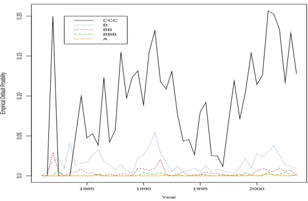
we will misreport the default rating, while quarterly data improves the accuracy but too few default events in quarterly period. After comparing these three different data structure, we choose semester-based period in this default study with GLMMs. The empirical default probabilities are presented in Figure 2.1. All the rating-categories have many defaults at the same time periods and followed by other periods with few defaults.

Year

Empirical Default Proability

1985 1990 1995 2000 0.0 0.05 0.10 0.15 0.20 CCC B BB BBB A

Figure 2.1: Empirical 6-month default rates for 23 years

The not-rated (NR) category in the S&P database is somewhat problematic. Some authors of empirical studies (e.g. Nickell et al. 2000) simply omit issuers who become NR from consideration. Other authors (e.g. Lando and Skoedeberg (2002)) treat transition to the not-rated category as a censoring event. Lando justifies this by citing evidence (Carty 1997) that the majority of transitions to not-rated are not related to changes in credit quality. In other words he argues that transition to not-rated is a non-informative censoring event, unrelated to the hazard of a firm subsequently

(46)

defaulting. There is also the issue that many NR firms subsequently regain a rating or are recorded as defaulting at a later date. Although we are ignorant about their true rating during the time that they are NR, it seems a pity to have to exclude them from a default analysis in particular.

We conducted the following analysis of the NR phenomenon. We considered all tran-sitions in the S&P database from ratings other than NR. We treated becoming NR as the event of interest and all other transitions (including default) as censoring events. We examined the covariates rating, country and sector. The conclusions: the lower rating categories have a significantly higher hazard of becoming NR than the higher rating categories; country has no discernable effect; tech firms have a significantly higher risk of becoming NR and utilities have significantly lower risk.

Thus the firms that become NR tend to be dominated by firms that have a higher default risk because they are lower rated. However, the question that is relevant from the point-of-view of the non-informative censoring assumption is whether a firm with a particular rating that becomes NR at a particular time point has a different default risk to a firm with the same rating that does not become NR? And there are many reasons to make a firm to become non-rated, including expiration of the debt, calling of the debt, failure to pay the requisite fee to S&P, etc. It is impossible for us to identify the exact reason for companies rating NR. Then we will treat NR case as censored in our analysis which means obligors whose rating isN Rhave been excluded from consideration but reconsider after they regain a rating.

The rating classes included in our analysis are

K={CCC, B, BB, BBB, A}

where we merge actual rating k+_{, k, k}− _into _k_{. We also merge} _{CCC, CC,} _and _C _into

a single rating class CCC. Rating classes AAA and AA which rarely default have been excluded from this study; they will be reconsidered in our transition analysis in the following chapters. More than 75% of the companies in the dataset from US, so

(47)

Sector Name #Observations 1 “Aerospace/automotive/capital goods/metal” 837 2 “Consumer/service sector”+“Transportation” 1355 3 “Energy and natural resources”+“Utility” 994 4 “Financial Institutions”+“Insurance”+“Real estate” 1666 5 “Hightec/computers/office equipment”+“Telecom” 628

6 “Leisure time/media” 670

Table 2.1: Numbers of industry sectors observations

we choose a subset of the dataset which consists of 6150 US companies from the 6 selected industry sectors in our definition, see Table 2.1:

The industry sectors in our analysis are slightly different from the S&P definition of industry sectors. We merged Consumer/service with Transportation, Energy with Utility, Financial institution with Insurance and Real estate, and finally High technol-ogy with Telecommunications. The industry sectors we merged have broadly similar business and may be supposed to be similarly impacted by macroeconomic covariates.

2.3.2 Results

Without considering obligor-level covariates, counterparties are grouped according to rating category. We include an observed macroeconomic variable to partly explain the time-heterogeneity in the default rates. Several macroeconomic variables including Chicago Fed National Activity Index (CFNAI)are used. This helps us to detect lags between the cycle of index and the actual default cycle.

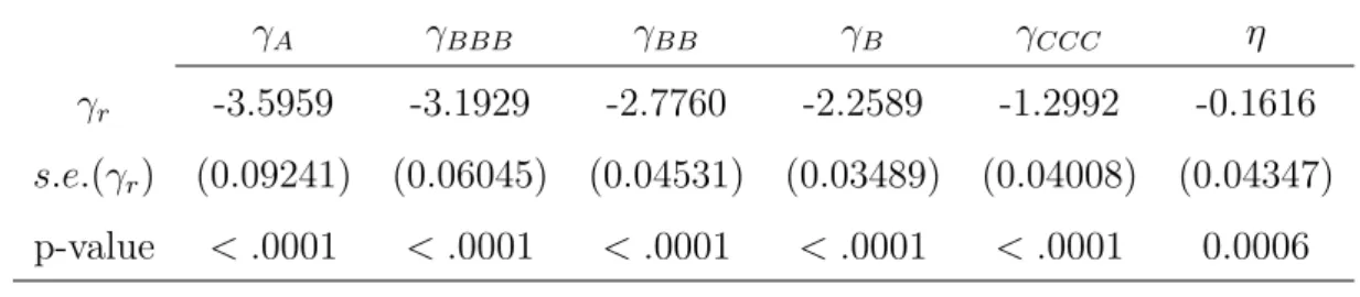
Model 2.1: One-factor model with Equicorrelation structure

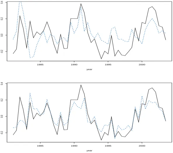
Let r = 1, . . . ,5 index the five rating categories in our study and γr is a fixed rating

effect. The rating class default probabilities are given by pr = Φ

γr √ 1+σ2 . The

Bayesian analysis of default and credit migration : latent factor models for event count and time-to-event data

Heriot-Watt University