An imprecise statistical method for accelerated life testing using the power-Weibull model.

(1)

Durham Research Online

Deposited in DRO:

30 May 2017

Version of attached le:

Accepted Version

Peer-review status of attached le:

Peer-reviewed

Citation for published item:

Yin, Y.-C. and Coolen, F.P.A. and Coolen-Maturi, T. (2017) 'An imprecise statistical method for accelerated life testing using the power-Weibull model.', Reliability engineering and system safety., 167 . pp. 158-167.

Further information on publisher's website: https://doi.org/10.1016/j.ress.2017.05.045

Publisher's copyright statement:

c

2017 This manuscript version is made available under the CC-BY-NC-ND 4.0 license http://creativecommons.org/licenses/by-nc-nd/4.0/

Additional information:

Use policy

The full-text may be used and/or reproduced, and given to third parties in any format or medium, without prior permission or charge, for personal research or study, educational, or not-for-prot purposes provided that:

• a full bibliographic reference is made to the original source • alinkis made to the metadata record in DRO

• the full-text is not changed in any way

The full-text must not be sold in any format or medium without the formal permission of the copyright holders. Please consult thefull DRO policyfor further details.

(2)

An imprecise statistical method for accelerated life

testing using the power-Weibull model

Yi-Chao Yin

Center for System Reliability and Safety, University of Electronic Science and Technology of China, Chengdu, Sichuan, China

Frank P.A. Coolen1

Department of Mathematical Sciences, Durham University, Durham, United Kingdom

Tahani Coolen-Maturi

Durham University Business School, Durham University, Durham, United Kingdom

Abstract

Accelerated life testing provides an interesting challenge for quantification of the uncertainties involved, in particular due to the required linking of the units’ failure times, or failure time distributions, at different stress levels. This paper provides an initial exploration of the use of statistical methods based on imprecise probabilities for accelerated life testing. We apply non-parametric predictive inference at the normal stress level, in combination with an estimated parametric power-Weibull model linking observations at different stress levels. To provide robustness with regard to this assumed link between different stress levels, we introduce imprecision by considering an interval around the parameter estimate, leading to observations at stress levels other than the normal level to be transformed to intervals at the normal level. The width of such intervals is increasing with the difference between the stress level at which a unit is tested and the normal level.

The resulting inference method is predictive, so it explicitly considers the random failure time of a future unit tested at the normal level. We perform simulation studies to investigate the performance of our imprecise predictive method and to get insight into a suitable amount of imprecision

(3)

for the linking between levels. We also explain how simulation studies can assist in choosing imprecision in order to provide robustness against specific biases or model misspecifications.

Keywords: Accelerated life testing, imprecise probability, lower and upper

survival functions, nonparametric predictive inference, power-Weibull model, right-censored data

1. INTRODUCTION

Testing of highly reliable units is often complicated if, under normal con-ditions, failures tend to occur only after a very long time, e.g. many years. This makes it hard, or even impossible, to infer aspects of the units’ failure time distribution at a relatively early stage, for example for comparison of units from different manufacturers. An effective way to still enable data

col-lection for such inferences is provided by so-called Accelerated Life Testing

(ALT), also known as accelerated stress testing, which is general terminol-ogy for a range of test scenarios, which have in common that units are tested under conditions that differ from the normal conditions. Under the changed conditions, the failure time distribution will change corresponding to reduc-tion of failure times, for example the voltage or temperature at which the units function may be increased for the tests. There is a wide variety of test designs, including constant stress testing, step stress testing and progressive stress testing. These test methods and a variety of statistical methods that can be applied for such methods are described in detail by Nelson [1].

In recent years, many methods have been developed for modelling and analysing ALT scenarios and data, we mention a few contributions to the rapidly increasing literature on ALT. Han [2] investigated constant-stress and step-stress ALT under time and budget constraints. Nasir and Pan [3] proposed a Bayesian optimal design criterion and planned ALT experiments for acceleration model selection. A Bayesian analysis for the Weibull pro-portional hazard model used in step-stress accelerated life testings was intro-duced by Sha and Pan [4]. In order to obtain a substantial amount of failure data within a reasonable period of time, Elsayed and Zhang [5] developed optimum multiple-stress-type ALT plans based on the proportional hazards

model. Mi et al. [6] discussed a reliability assessment method for ALT on

complex electromechanical systems with field data affected by multiple fac-tors. Mukhopadhyay and Roy [7] present Bayesian methods for multi-stress

(4)

ALT on series systems. In this paper, we consider a basic ALT scenario using a power-Weibull model to combine information from units tested at constant stress levels, where we aim at prediction of the failure time for a future unit at the normal stress level.

Constant stress testing is a basic and widely used ALT design. The

units are divided into several groups and all units in a group are tested at a constant stress level. In this paper we only consider this relatively straight-forward form of ALT. The research reported forms the first part of a long term research project to develop a range of ALT methods using imprecise statistical approaches, where in particular the links between different stress levels are typically quite uncertain and hence there may be benefit in using imprecision in the modelling of these links. The main challenge for statistical methods for ALT lies in the obvious fact that information from a test with increased stress levels must be transformed to information that can be con-sidered as representative for information about units’ failure times under the normal conditions. Due to the practical relevance of ALT and the obvious challenges for statistical inference based on ALT data, many statistical mod-els and methods for ALT data have been presented [1]. A standard model for failure time data resulting from ALT is the power-Weibull model, which we considered as the first stage in our research and which we explore in this paper.

The power-Weibull model [1] consists of a Weibull model for failure times

at stress leveli= 0,1,2, . . . , k, where leveli= 0 is the normal level and levels

i= 1,2, . . . , k representkincreased stress levels. These Weibull distributions

for different stress levels are assumed to have the same shape parameter β,

but different scale parametersαi. Assuming that the stress level is quantified

by a single positive measurement Vi for stress level i, which is an increasing

function of the stress level i (one can e.g. think of voltage), the different αi

values are assumed to satisfy the equation

αi =α V0 Vi p (1)

such that α0 = α is the Weibull scale parameter at the normal stress level

and pis the parameter of the power-law which models the link between the

Weibull distributions at different stress levels. For clarity, in this paper we

(5)

and scale parameter α corresponding to the survival function P(T > t) = exp ( − t α β) (2) A useful alternative way to understand this power-law link between the dif-ferent stress levels is provided by the fact that, under this model assumption,

an observation ti _{at stress level} _i_{, so subject to stress} _V

i, can be interpreted

as being transformed to an observation

ti→0 =ti Vi V0 p (3) at stress level 0. It should be remarked here that, in this initial investigation,

we assume the same shape parameter β for all stress levels Vi. This

assump-tion can be relaxed, in which case the method can still be applied with a relatively straightforward transformation formula for the observations from

level i to level 0.

As the objective of ALT is, obviously, to have a reduction of failure times

at higher stress levels, it is natural to assume that p > 0, with p > 1 most

likely in practical applications. Given failure time data, which can contain right-censored data under the usual assumption that the cause of censoring holds no information about the remaining future time to failure of a unit

for which only a right-censored observation is available, the parameters α,

β and p of this model can be straightforwardly estimated by maximising

the likelihood function, which requires a numerical optimisation method; computations in this paper were performed with the statistical software R.

Section 2 of this paper provides a short introduction to nonparametric predictive inference (NPI), in particular it provides the NPI lower and up-per survival functions for a future observation based on failure time data including right-censored observations, these are used in the new statistical method for ALT data which is presented in Section 3. This new method consists of two stages. In the first stage, the power-Weibull model is as-sumed for the observations at all stress levels simultaneously, including the

parameter p representing the link between different stress levels. Based on

all the data, the parameters in this model are estimated using maximum likelihood estimation. In the second stage, only the point estimate for the

link parameter p is used to transform data from the different stress levels

(6)

lower and upper survival functions for the next unit at the normal stress level. In Section 4 this approach is extended by including imprecision in the link parameter, which leads to observations at levels other than the normal stress to be transformed to interval-valued observations at the normal stress level. The width of these intervals increases as function of the difference between the corresponding stress level and the normal stress level. These interval-valued observations are then used in the NPI approach to lead to new lower and upper survival functions with increased imprecision. This can be interpreted as a straightforward method to provide robust predictive infer-ences based on ALT data. This is the first investigation towards developing NPI methods for ALT data, the general idea of using imprecision as a safe-guard against lack of detailed knowledge in ALT settings seems attractive. In Section 5 we present the results of an initial simulation study, which is the first step towards investigating and further developing our approach. In these simulations we investigate the method’s performance for the case that data are actually simulated from the assumed power-Weibull model, hence only parameter estimation and the connection with NPI for prediction at the standard stress level are investigated. In Section 6 we briefly discuss the use of imprecision in our method to provide robustness with regard to possible model misspecification. Section 7 provides brief concluding remarks about the proposed method and the future work planned in this research project.

Before we begin the presentation of our inferential method, it is impor-tant to provide some additional explanation of the aims of our research, both as presented here and the longer term research project, for the ben-efit of real applications of ALT. As ALT scenarios are typically complex and require some level of extrapolation from observable data, they provide huge challenges for modelling and statistical inference. There seems to be a tendency, in the literature, for ever more complicated and detailed models. While of theoretical interest, we expect that practitioners may be helped by an opposite approach, namely by development of relatively straightforward statistical models and methods with built in robustness, hence with quite wide applicability but at a price, namely that inferences are not expressed through precise probabilities but through intervals of probability values. If such intervals do not provide clear answers to practical problems, then once can still consider adding modelling assumptions, gathering more data, or in-clude expert judgements in order to reach an overall answer. We consider that this has advantages over methods based on very detailed mathematical assumptions if these cannot be verified or justified, but of course one could

(7)

also perform analysis with a robust method like the one we present here as well as with more detailed models, where comparison of results provides use-ful insights into the influence of the additional assumptions underlying the more complicated models. If one has detailed knowledge to justify compli-cated models, e.g. based on materials science or physics, then of course it is beneficial to use this knowledge, and we would also advocate it to be imple-mented in an approach like ours. However, in absence of such knowledge the use of very detailed models may lead to misspecification without clarity of its influence on the final results. We suggest that ideas about possible differ-ences to an assumed model, so biases or even possibly different models, can be included in our method through simulation studies, aiming at sufficient imprecision so that our imprecise results also cover for the suggested range of misspecifications.

Statistical inference is traditionally in terms of ‘populations’, infinite num-bers of ‘identical’ items would be used of which one tests a sample. Our approach, as presented here, is predictive and considers only a single future item. Of course, this represents all future items, but if one would wish to de-velop such methods explicitly for multiple future items, then this brings with it some complications if one has relatively few data, because the failure times of the future items would not be mutually conditionally independent given the failure data (NPI for multiple future observations has been developed for other statistical settings, but not yet in relation to the methods presented here). As most practical problems probably involve multiple future items of interest, but not necessarily an infinite population, both approaches could be seen as somewhat artificial, mainly to facilitate development of statistical methods. We think that for example comparison of two types of lightbulbs in terms of an event of the kind ‘a future lightbulb of Type A will fail before a future lightbulb of Type B’ may be attractive, this is the sort of event we have in mind in this overall research project.

2. Nonparametric predictive inference

Nonparametric predictive inference (NPI) is a statistical method based

on Hill’s assumptionA(n) [8], which gives a direct conditional probability for

a future observable random quantity, given observed values of related

ran-dom quantities [9, 10, 11, 12]. Let Y1, . . . , Yn, Yn+1 be positive, continuous

and exchangeable random quantities representing event times [13]. Suppose

(8)

ob-served values are denoted by 0 < y1 < . . . < yn < ∞, for ease of notation

let y0 = 0 and yn+1 = ∞. For ease of presentation, it is assumed that no

ties occur among the observed values. It is quite straightforward to deal with tied observations in this setting, by assuming that tied observations

differ by small amounts which tend to zero. For the random quantity Yn+1

representing a future observation, based on n observations, the assumption

A(n) [8] is P(Yn+1 ∈ (yi−1, yi)) = 1/(n + 1) for i = 1, . . . , n+ 1. A(n) does

not assume anything else, and can be interpreted as a post-data

assump-tion related to exchangeability [13]. Inferences based on A(n) are predictive

and nonparametric, and can be considered suitable if there is hardly any

knowledge about the random quantity of interest, other than the n

observa-tions, or if one does not want to use such information, e.g. to study effects

of additional assumptions underlying other statistical methods. A(n) is not

sufficient to derive precise probabilities for many events of interest, but it provides bounds for probabilities via the ‘fundamental theorem of probabil-ity’ [13], which are lower and upper probabilities with strong consistency properties in the theory of imprecise probability [9, 14].

In reliability analyses, events of interest are often failures of units, but failure time data may be affected by right-censoring, where for a unit it is only known that it has not yet failed by a specific time. Coolen and Yan [15]

presented a generalization of A(n), called ’right-censoring A(n)’ or rc-A(n),

which is suitable for NPI with right-censored data and uses the additional assumption that, at the moment of censoring, the residual time to failure of a right-censored unit is exchangeable with the residual times to failure of all other units that have not yet failed or been censored. This is a clear formulation of the common ‘non-informative censoring’ assumption, which is therefore assumed throughout this paper if there are right-censored data. It should be mentioned that this assumption is quite standard for application of Maximum Likelihood Estimation, or other estimation methods, for ALT data, as used for parameter estimation in this paper. For ALT, test designs with a pre-fixed maximum testing time are frequently used; in such cases the censoring is non-informative according to the description given above, hence the presented method can be applied in case of censored data resulting from such experiments.

Suppose that there are n observations consisting of ufailure times, x1 <

x2 < . . . < xu, and n−u right-censored observations, c1 < c2 < . . . < cn−u.

Let x0 = 0 and xu+1 =∞. Suppose further that there are si right-censored

(9)

Pu

i=0si = n −u. We introduce notation d

i

j for any observation, either a

failure or right-censoring time, with di₀ =xi anddji =cij forj = 1, . . . , si and

i = 0,1, . . . , u. Let ˜ncr and ˜ndi

j be the number of units in the risk set just

prior to time cr and dij, respectively, with the definition ˜n0 =n+ 1 for ease

of notation. Let di_si₊₁ = di₀+1 = xi+1 for i = 0,1, . . . , u−1, and note that

the product taken over an empty set is defined as equal to one. Based on

the assumption rc-A(n) [15], the NPI lower and upper survival functions for

the failure time of the next unit, S_Xn+1(t) and SXn+1(t), respectively, are as

follows [16, 17]. For t∈[di j, dij+1) with i= 0,1, . . . , u and j = 0,1, . . . , si, S_Xn+1(t) = 1 n+ 1 n˜dij Y {r:cr<di j} ˜ ncr + 1 ˜ ncr (4)

and for t ∈[xi, xi+1) withi= 0,1, . . . , u,

SXn+1(t) = 1 n+ 1 ˜nxi Y {r:cr<xi} ˜ ncr + 1 ˜ ncr (5)

These NPI lower and upper survival functions are step-functions, presented in product forms which lead to relatively straightforward computation. Note that the Kaplan-Meier (KM) estimate [18] based on such data, which is the classical nonparametric maximum likelihood estimate, always lies between the NPI lower and upper survival functions [15]. Whilst the KM estimate has also been used for ALT data [1], it should be emphasized that its explicit aim is estimation of an underlying population distribution, whilst our NPI approach is explicitly predictive and considers events involving one future observation at the normal stress level.

The lower and upper survival functions (4) and (5) fit well into the theory of imprecise probability [14]. The imprecision in these inferences, that is the difference between corresponding upper and lower survival functions, results from the limited inferential assumptions made and reflects the amount of information in the data. Note, for example, that the upper survival function only decreases at an observed failure time, while the lower survival function decreases both at an observed failure time and, by a smaller amount, at a right-censored observation. This is in line with a useful, albeit somewhat informal interpretation of imprecise probabilities, namely that a lower prob-ability reflects the information in favour of the event of interest, and the

(10)

difference between 1 and the corresponding upper probability reflects the in-formation against the event of interest. So the decrease of both the NPI lower and upper survival function at an observed failure time reflects a decrease of information supporting survival past this time, while a right-censored obser-vation reduces the information in favour of survival (hence the slight decrease of the lower survival function) but does not provide evidence against survival (so the upper survival function is not affected).

3. NPI with estimated link

The new statistical method for ALT data, which we propose in this pa-per, consists of two stages. In the first stage, the basic power-Weibull model is assumed and its parameters are estimated using maximum likelihood esti-mation. The Weibull probability density function is

f(ti) = β αi (t i αi )(β−1)exp(−(t i αi )β) (6)

where αi > 0 is the Weibull scale parameter at stress level i and β > 0 is

the Weibull shape parameter. By substituting the power-law link function (1) into (6) we obtain the accelerated life test model with probability density

function at level i= 0,1. . . . , k equal to

f(ti) = β α(V0_Vi)p( ti α(V0_Vi)p) (β−1) exp(−( t i α(V0_Vi)p) β ) (7)

where level 0 represents the stress level under normal circumstances, hence interest is particularly in inferences at this level. As mentioned, this is the first proposal of an NPI-based imprecise model for accelerated test scenarios. Other models can be used instead of this power-Weibull model, as well as other estimation methods; these are aspects that will be explored later in this research project. This first stage uses maximum likelihood estimation, based on failure data (possibly including right-censored observations) at the different stress levels, and results in point estimates for the three parameters

α, β and p. However, at the next stage only the estimate for p is used, we

denote this by ˆp. In the second stage, we transform all observations at stress

levels other than the normal level, so V1, . . . , Vk, to ‘equivalent’ observations

(11)

given by Equation (3), leading to transformed observations ti Vi V0 pˆ

Right-censored observations are transformed similarly, where their status as right-censored observation is maintained. Now, we apply NPI with all these

transformed data as well as the original data at the normal stress level V0,

as explained in Section 2. We illustrate the results of this approach in an example using data from the literature; this example will also be used for an extension of this method in Section 4.

Example

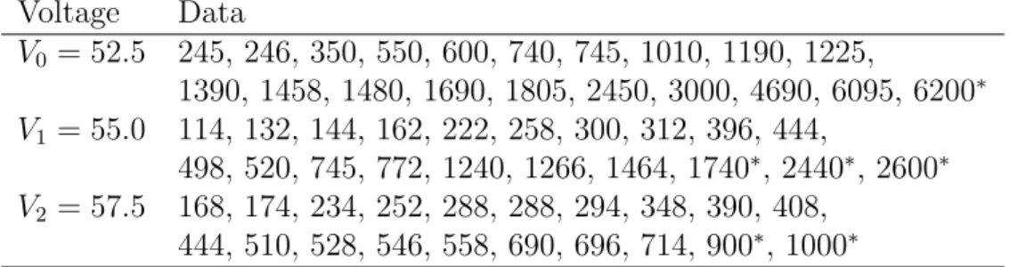
Lawless [19, p.341] presents the ALT data set below in an exercise with further reference to an unpublished Master’s thesis. The data result from an experiment in which specimens of solid epoxy electrical insulation were studied in an accelerated voltage life test. Twenty specimens are tested at

each of three voltage levels, the normal level V0 = 52.5 and increased levels

V1 = 55.0 and V2 = 57.5 kilovolts. Most of the sixty specimens actually

failed during the experiments, but a few did not, these provide right-censored observations. The failure times, in minutes, are given in Table 1, where a right-censored observation is indicated with a superscript asterisk.

Table 1: Failure times at three voltage levels.

Voltage Data V0 = 52.5 245, 246, 350, 550, 600, 740, 745, 1010, 1190, 1225, 1390, 1458, 1480, 1690, 1805, 2450, 3000, 4690, 6095, 6200∗ V1 = 55.0 114, 132, 144, 162, 222, 258, 300, 312, 396, 444, 498, 520, 745, 772, 1240, 1266, 1464, 1740∗, 2440∗, 2600∗ V2 = 57.5 168, 174, 234, 252, 288, 288, 294, 348, 390, 408, 444, 510, 528, 546, 558, 690, 696, 714, 900∗, 1000∗

Maximum likelihood estimation for the power-Weibull model, based on

these data, leads to parameter estimates ˆβ = 1.183, ˆα = 2038.790 and ˆp =

15.09927. These estimates imply ˆα0 = 2038.790, ˆα1 = 1009.988 and ˆα2 =

516.205. It should be remarked that the numerical maximum likelihood

optimisation to derive these estimates in the statistical software R appears to be somewhat sensitive to the starting point of the algorithm, we noticed

(12)

some slight variation in the resulting estimates for different starting points. We discuss this aspect briefly in the concluding remarks section, the variation

observed in the estimate ˆp was small and will not affect our approach as

proposed in this paper, in particular as we will later include imprecision for this estimate.

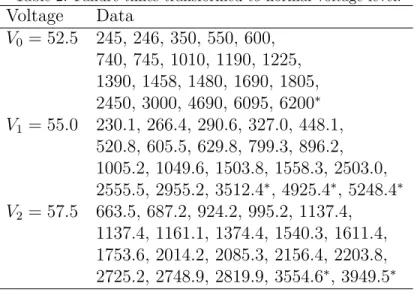
In the second stage of our procedure, we only use the estimate ˆpto

trans-form the data, as explained above. This leads to the transtrans-formed data values in Table 2, still listed with their corresponding stress level. Of course, the

data at the normal stress levelV0 = 52.5 have not been transformed, but are

also included in the table for ease of comparison with the transformed data from the other stress levels. These transformed data are also presented in Figure 1, where the transformations of the data from the stress levels 1 and 2 to the normal level 0 are illustrated.

Table 2: Failure times transformed to normal voltage level.

Voltage Data V0 = 52.5 245, 246, 350, 550, 600, 740, 745, 1010, 1190, 1225, 1390, 1458, 1480, 1690, 1805, 2450, 3000, 4690, 6095, 6200∗ V1 = 55.0 230.1, 266.4, 290.6, 327.0, 448.1, 520.8, 605.5, 629.8, 799.3, 896.2, 1005.2, 1049.6, 1503.8, 1558.3, 2503.0, 2555.5, 2955.2, 3512.4∗, 4925.4∗, 5248.4∗ V2 = 57.5 663.5, 687.2, 924.2, 995.2, 1137.4, 1137.4, 1161.1, 1374.4, 1540.3, 1611.4, 1753.6, 2014.2, 2085.3, 2156.4, 2203.8, 2725.2, 2748.9, 2819.9, 3554.6∗, 3949.5∗

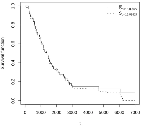
Using these 60 (tranformed) failure observations at the normal stress level

V0, so both the originally observed data at levelV0 and the data transformed

to it from stress levels V1 and V2, the NPI approach as described in Section

2 provides NPI lower and upper survival functions presented in Figure 2,

where we used the estimate ˆp= 15.09927 for the link function. These lower

and upper survival functions are to be interpreted as applying for a further specimen, exchangeable with those in the test, subjected to the normal stress

level V0 = 52.5, with the explicit assumption that the transformed data from

(13)

0 1000 2000 3000 4000 5000 6000 50 52 54 56 t0 y0

Figure 1: Transformed data using ˆp

V0, so that indeed the future observation of interest can be assumed to be

exchangable with all 60 (transformed) observations at level V0.

4. Imprecision in link estimate

The method presented in Section 3 has several aspects which can cause doubt about the validity of the predictive inference. These include doubt about the model used at stage 1 and, related to this, the fact that the esti-mation of the Weibull parameters influences the estimate of the parameter

ˆ

p but is further neglected at stage 2. As mentioned in the example, there

may also be some numerical instability in the estimation computations and it has been reported that maximum likelihood methods for such accelerated life test data can lead to bias in the estimates when relatively small sample sizes are used [20]. One could rebute all such issues by suggesting more detailed modelling, but particularly for ALT data there often remains an element of model-based extrapolation that is difficult, sometimes even impossible, to justify on the basis of available data.

We propose a different approach as an alternative to more detailed mod-elling, although if such modelling can be done on the basis of detailed knowl-edge of the scenario under study then, of course, this is strongly recom-mended; it can still be worth combining more detailed modelling with the new ideas we present in this paper. In an attempt to develop suitable pre-dictive inference for ALT data, where interest is in the failure time of a future unit at the normal stress level, we propose to adapt the two stage

(14)

0 1000 2000 3000 4000 5000 6000 7000 0.0 0.2 0.4 0.6 0.8 1.0 t Sur viv al function Sp=15.09927 Sp=15.09927

(15)

approach presented in Section 3 by replacing, in the second stage, the point

estimate ˆp by an interval [p, p] which contains ˆp. The use of this interval in

the transformation of observations at stress level Vi to the normal level V0

leads to such observations becoming interval-valued observations at the nor-mal stress level, which we believe is an attractive way for showing the effect of imprecision in line with the absence of perfect information about the link between the different stress levels. Furthermore, these intervals representing

observations at other levels will be wider for larger values of i, so an original

observation from a stress level that is further away from the normal level is transformed to a wider interval at the normal level than an original observa-tion at a level nearer to the normal level. We believe that, in general, this is also an attractive property of such imprecise inferences for ALT data. In fact, we were quite surprised when studying the literature on ALT that such imprecise statistical methods apparently had not yet been used, we regard this as an important contribution of the current paper, which presents our first results for inferences with ALT data from this perspective and is the start of a research project in which we are considering both alternatives to the statistical modelling and other ALT scenarios, we comment further on this in Section 7.

Due to the monotonicity of the transformed data in the power-Weibull

model as function of the parameter p, together with the monotonicity of the

NPI lower and upper survival functions with regard to the data on which

they are based, an interval [p, p] straightforwardly leads, in the second stage

of our method, to the NPI lower survival function being based on the

trans-formed data usingp, and the NPI upper survival function being based on the

transformed data using p. Hence, the imprecision in this inferential method,

that is the difference between the corresponding NPI upper and lower

sur-vival functions, will increase when the width of the interval [p, p] increases,

which is illustrated in the following example. The important question of how

to choose an interval [p, p] in practice is considered in the remainder of this

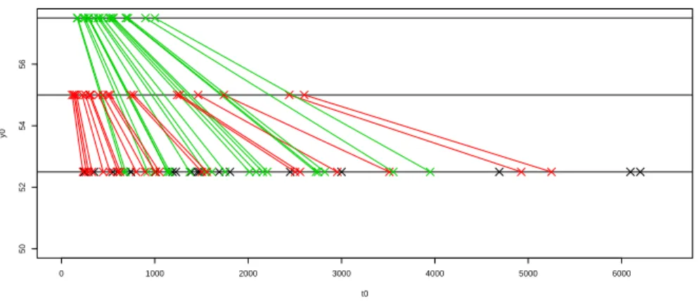
paper, and is also an important topic for further research. Example (ctd)

For the example in Section 3, the point estimate for p was equal to ˆp =

15.09927, the NPI lower and upper survival functions corresponding to this

value were presented in Figure 2. Figure 3 presents the NPI lower and

upper survival functions corresponding to intervals [p, p] for the parameter

(16)

0 1000 2000 3000 4000 5000 6000 7000 0.0 0.2 0.4 0.6 0.8 1.0 t Sur viv al function Sp=20 Sp=17 Sp=15.5 Sp=14.5 Sp=13 Sp=10

Figure 3: NPI lower and upper survival functions for [p, p] = [14.5,15.5]; [13,17]; [10,20]

shows that increased imprecision for the parameter p leads to increased

dif-ferences between the NPI upper and lower survival functions. It is interesting

to see that even for very substantial imprecision forpthe imprecision between

the lower and upper survival functions is mostly not too large. Of course,

this depends on the ratiosVi/V0 used, which are close to one in this example,

but nevertheless it suggests that some concerns, e.g. about some sensitivity to the starting point of the numerical optimisation methods used to derive

ˆ

p, are not necessary. It should be emphasized that this example is included

to illustrate the increasing imprecision in the NPI lower and upper survival

functions due to increasingly wide intervals forp. Methods for suitable choice

of such an interval in practice are discussed later, and will also be addressed in future research.

5. Simulations

This paper presents first ideas and results of a research project towards developing powerful predictive statistical methods for ALT data, based on few modelling assumptions and ideas related to imprecise probabilities [14]. To gain first insights, we performed simulations to investigate if the approach works if the assumed power-Weibull model is actually the true underlying model, hence with data simulated from this model.

(17)

For this first simulation, we set stress levels V0 = 50, V1 = 80, V2 = 120

and parameters α = 1500, β = 3 and p = 10 for the power-Weibull model.

We ran 10,000 simulations with n= 10 observations at each stress level per

run. We used the MLE method within the statistical software R to estimate

the parameters, then used the ˆpfor the transformation of the data from stress

levels V1 and V2 to the normal stress level V0. This leads to 30 observations

at the normal stress level, 20 of which are transformed from higher stress levels. In addition, per run we simulated one more observation at the normal stress level, this serves as ‘future observation’ and is needed to investigate the predictive performance of our method, which we do as follows.

If the model fits well, in particular the link transforming observations between different stress levels, then we can consider all 30 (transformed) ob-servations just as if they were actually obob-servations at the normal stress level. In this case one would expect good mixing of these 20 transformed obser-vations and the 10 actual obserobser-vations at the normal stress level, which can be investigated as follows. First, restricting to the actual 10 observations at the normal stress level, these partition the positive real-line into 11 intervals (assuming no tied observations), the further simulated future observation at this level will have equal probability to be in each of these intervals. So, if we perform many simulations, this future observation will be in each of the 11 intervals roughly in 1/11 of the simulation runs. Now considering the 30 observations after transforming the 20 from the higher stress levels. If the transformation is perfect, so that indeed we can consider the 20 transformed data observations as if they really represent data at the normal stress level, then we can consider the location of the ‘future observation’, sampled at the normal stress level, as being exchangeable with all the 30 observations. So we can consider the partition of the positive real-line into 31 intervals (assuming again that there are no tied observations, also not after the transformation)

created by the 30 observations at stress level V0, and the future observation

should now have equal probability 1/31 to fall into each of these 31 inter-vals. Therefore, each run in the simulation study consists of generating 10 observations at each stress level, estimating the parameters, using the MLE

ˆ

p to transform the data from stress levels V1 and V2 to level V0, and then

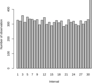
checking in which of the 31 intervals the further simulated ‘future observa-tion’ is. If, over many runs, this interval is reasonably uniformly distributed, then the method works well as it indicates that the 20 transformed data in-deed are well mixed with the original 10 observations at the normal stress level. If, however, there are different patterns, then it indicates non-perfect

(18)

1 3 5 7 9 12 15 18 21 24 27 30 Interval Number of obser v ation 0 100 200 300 400

Figure 4: Intervals of next observation withn= 10

mixing which will lead to doubt about the transformation applied between the different stress levels.

Figure 4 shows a histogram presenting the frequencies with which this future observation belonged to each of the 31 intervals in the 10,000 sim-ulation runs. This histogram suggests reasonable uniformity, but there are clearly too many runs for which it falls into the final interval. This indicates

that the transformed data from stress levels V1 and V2 were not sufficiently

often greater than the largest observation from level V0, and hence a slight

tendency for the MLE method to under-estimate ˆp. Further investigation

revealed that indeed this is the case, with the estimate ˆp being a bit less

than 10 in most simulation runs. We repeated this simulation several times, always leading to the same conclusion. It should be remarked that bias in parameter estimates for ALT models has been reported previously [20], we briefly discuss this further in Section 7.

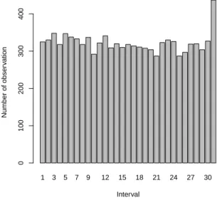
Figure 5 shows the results of the same process but now with the parameter

β = 3, as used in the simulations, assumed known in the fitted model, hence

only the parameters α and p are estimated by the MLE method. This has

very little effect compared to the previous case where β was also estimated,

(19)

Figure 5: Intervals of next observation withn= 10 andβ= 3

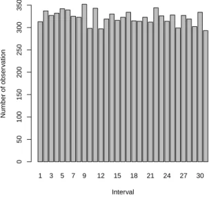
of p. Figure 6 shows the results with bothα= 1500 and β = 3 fixed, so only

pestimated. This leads to a better fit with the expected uniform distribution

over the 31 intervals, as was also confirmed in repeated simulations for this

case. This illustrates that the slight bias in ˆpresults from the joint estimation

of multiple parameters of the model when the maximum likelihood method

is used, where in particular the joint estimation of α and p causes some

problems. We also investigated this for smaller and larger simulated sample

sizes. For smaller values ofnthe same effect is even stronger, while forn = 20

it is quite reduced, and for larger sample sizes the bias due to the estimation process becomes neglectable. Of course, in reality we have to include all model parameters in the estimation process, so we suggest a different way for dealing with such possible bias, namely through replacement of the use

of a single estimate ˆp, for the predictive inference in the second stage of our

method, by an interval of values for the parameter p.

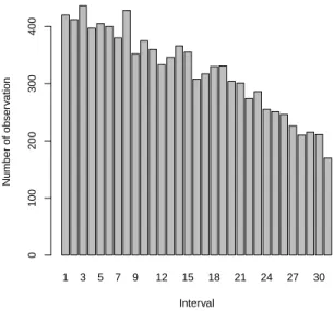
We next investigate the effect of replacing the estimate ˆp for the data

transformation with a slightly changed value. As we noted above that there

was a tendency to slightly under-estimate the value of p, we instead use the

value 1.02×pˆ for the data transformation from levels V1 and V2 to V0 in

(20)

1 3 5 7 9 12 15 18 21 24 27 30 Interval Number of obser v ation 0 50 100 150 200 250 300 350

Figure 6: Intervals of next observation withn= 10,β = 3 andα= 1500

given in Figure 7. Note here that, due to the substantial difference in the

values V0, V1, V2 in this example, this small factor with which the value for

p is multiplied already makes a substantial difference to the factors used for

the transformation of data to the standard stress level. This figure shows a quite different result to the earlier figures, with a decreasing trend over the intervals. This shows that the transformed data are now a bit too large, as they do not add sufficient intervals to the partition of the positive real-line

among the smaller actual observations at stress level V0. For completeness

of the study, Figure 8 shows the similar histogram with the value 0.98×pˆ

used for the data transformation. This leads to the transformed data at

stress level V0 being smaller than with the use of ˆp, the effect of the bias to

this estimate is even more emphasized. This basic simulation study suggests that, while the predictive method may not work very well for smaller data

sets when a single value for p is used for the data transformation, the use

of an interval of values for p in the transformation process may cover a

range of different prediction results, which we would aim to include cases of reasonable uniformity. In the above case, we could e.g. opt to use the interval

[p, p] = [ˆp,1.02×pˆ] or [p, p] = [0.98×p,ˆ 1.02×pˆ]. To illustrate this further,

(21)

Figure 7: Intervals of next observation withn= 10 andp= 1.02×pˆ

values ˆp, 0.98×pând 1.02×pˆ, also the values 0.9×pând 1.1×pâre used.

These latter two values clearly lead to the transformed data being too small or too big, respectively, compared to the actual data at the standard stress level and the future observation at that level. However, if we were to use the

interval [p, p] = [0.9×p,ˆ 1.1×pˆ] in our proposed inference method, it would

provide considerable robustness against bias in estimation or other reasons why one may doubt the use of the model.

The NPI inferences for a future observation at the normal stress levelV0,

as presented in this paper, using such an interval of values for p, provide

a level of robustness. It makes sense to aim at a relatively small interval

for p in order to keep the imprecision small. Balancing this choice with the

provided robustness is a topic for future research, it also depends on levels of possible model misspecification against which one would hope to provide sufficient robustness, this is briefly considered in Section 6.

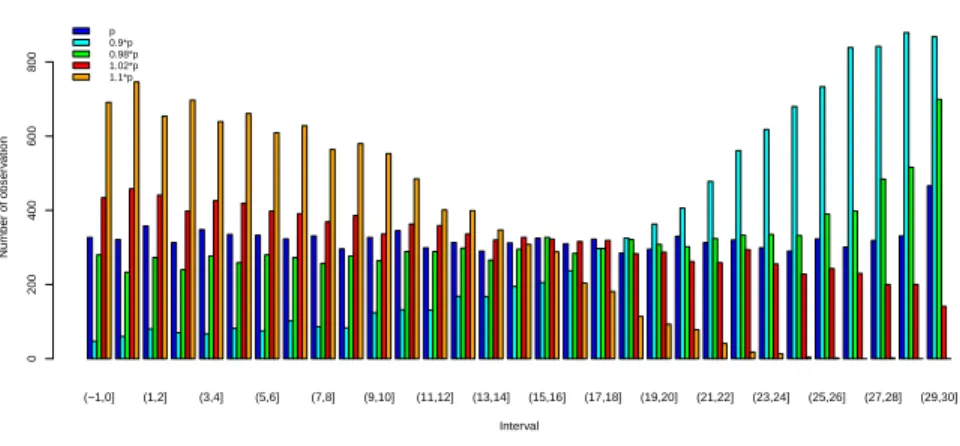
For the investigation into the performance of our new predictive inference method for ALT data it is of interest to perform simulations as presented above, checking the overall fit by considering a future observation at the normal stress level and how it mixes among all the actual data, after their transformation to the normal stress level. However, one may only be

(22)

inter-1 3 5 7 9 12 15 18 21 24 27 30 Interval Number of obser v ation 0 100 200 300 400 500 600 700

Figure 8: Intervals of next observation withn= 10 andp= 0.98×pˆ

(−1,0] (1,2] (3,4] (5,6] (7,8] (9,10] (11,12] (13,14] (15,16] (17,18] (19,20] (21,22] (23,24] (25,26] (27,28] (29,30] p 0.9*p 0.98*p 1.02*p 1.1*p Interval Number of obser v ation 0 200 400 600 800

(23)

ested in one or a few specific inferential questions, for example in the quartiles of the NPI lower and upper survival functions, and whether or not the fu-ture observation exceeds these quartiles in the right proportion out of 10,000 simulations. We performed similar simulations as before in this section, but now for each run checking whether or not the simulated future observation exceeds the first, second and third quartiles corresponding to both the NPI lower and upper survival functions based on the simulated data, consisting

of n observations at each of the three stress levels. We considered the effect

of varying the number of observations by taking n = 10,20,30, the results

are presented in Figures 10, 11 and 12, respectively. In these simulations, the NPI lower and upper survival functions are only using the MLE estimate

ˆ

p, so we have not included further imprecision by using an interval of values

for p; we earlier noticed some bias when doing this, but mainly in the final

interval, so it may still function well when we are considering the quartiles.

In these figures, qL0.25 and qU0.25 denote the first quartiles corresponding

to the NPI lower and upper survival functions, respectively, and so on. If the method works perfectly well, the future observation at the normal stress level should exceed this first quartile of the NPI lower survival function in just over 75% of all simulation runs, and the first quartile of the NPI up-per survival function in just under 75% of the runs, and similarly for the second and third quartiles (50% and 25%). Figures 10-12 show that these proportions are indeed achieved, which indicates good performance of our method when interest is in the quartiles. Note that the differences between corresponding proportions for the upper and lower survival functions tend to

decrease for larger values of n, which reflects that the NPI lower and upper

survival functions are closer to each other when based on more observations. Again, repeats of these simulations resulted in the same conclusions.

The basic simulation study reported in this section has provided some relevant insights, namely that the method works quite well in the sense of providing suitable predictive inference in case the data actually come from the general model class assumed, with possibly a slight bias in the estimation

of the parameterpof the function used for transformations between different

stress levels. The use of an interval of values forp, instead of a point estimate,

provides robustness against such bias. A perhaps more important reason to

choose an interval of values for p is to reflect that the assumed model, and

particularly the function linking the different stress levels, will normally not be entirely accurate for the real world scenario. A logical question therefore

(24)

qL0.25 qU0.25 qL0.5 qU0.5 qL0.75 qU0.75 0.0 0.2 0.4 0.6 0.8 1.0 0.7705 0.739 0.5134 0.482 0.267 0.2363

Figure 10: Proportion of runs with future observation greater than the quartiles,n= 10

qL0.25 qU0.25 qL0.5 qU0.5 qL0.75 qU0.75

0.0 0.2 0.4 0.6 0.8 1.0 0.7501 0.7345 0.5005 0.4871 0.2602 0.2415

(25)

qL0.25 qU0.25 qL0.5 qU0.5 qL0.75 qU0.75 0.0 0.2 0.4 0.6 0.8 1.0 0.7593 0.748 0.5068 0.4953 0.2504 0.2405

Figure 12: Proportion of runs with future observation greater than the quartiles,n= 30

this in the following section.

6. Misspecification of the model

Among the many challenges for statistical methodology for ALT data and inferences [21, 22], an obvious one is dealing with possible misspecification of the model. The ultimate aim of our research program is development of pre-dictive inference methods based on few modelling assumptions, with included robustness against the necessary assumptions, which include modelling the link between different stress levels.

For the first steps in this program, as reported in this paper, one can

consider the choice of the interval [p, p] in order to have a suitable level

of robustness against some specific differences to the model. To illustrate

this, we simulate data for the same scenario as in Section 5, with n = 10

observations at each of the three stress level. But now we simulate from a model that differs from the power-Weibull model assumed for the analysis, yet given the simulated data we follow the same approach as in Section 5.

After simulating the data at stress levels V0, V1 and V2, we added some

(26)

We present the results for the scenario where these random noises are Exponentially distributed, for three cases with the following rate parameters:

(1) for observations at V1 we use rate 0.5 and forV2 rate 10; (2) rates 0.7 and

12, respectively; (3) rates 0.9 and 14, respectively. Using these simulated observations, so with the bias added at the two increased stress levels, we applied our method as before, so we computed the MLE for the parameters

α, β, pfor the power-Weibull model, then used the MLE ˆpfor the second stage

of our method. To achieve robustness we used the interval [0.98×p,ˆ 1.02×pˆ]

to derive the NPI lower and upper survival functions.

The results of these simulations, again showing the intervals in which

the simulated future observations at levelV0 fall, are presented in Figure 13.

Such a plot provides an insight into whether or not our method provides suitable robustness against the particular misspecification case considered. If the smallest and largest numbers of the future observations per interval in

this plot tend to correspond to the cases with the use of 0.98×pˆor 1.02×pˆ,

then our imprecise method provides sufficient robustness for inferences not to be affected by the simulated misspecification. We ran further simulations with comparable small biases sampled from other distributions, these led to the same results. Of course, if one increases the biases, one would need

to use a larger interval of values for p. Furthermore, one may wish to study

misspecifications of different natures, e.g. including simulating data from one or more different ALT models than the power-Weibull model assumed for the

inferences. Suitable choices for the interval of values for the parameter pcan

still be studied, for such cases, through simulations as performed in this section.

7. Concluding Remarks

This paper has presented an initial study of possibilities provided by theory of imprecise probabilities and imprecise statistics approaches [14] for ALT applications. The proposed method combines transformation of fail-ure times at increased stress levels to equivalent observations at the normal stress level, based on an assumed fully parametric model, with nonparamet-ric predictive inference based on all the combined data at the normal stress level. The method provides the attractive opportunity to build in robustness for the inferences through the use of an interval of values for the parameter of the link function between different stress levels, which has the effect that an observation transformed from a higher stress level becomes an

(27)

interval-(−1,0] (1,2] (3,4] (5,6] (7,8] (9,10] (11,12] (13,14] (15,16] (17,18] (19,20] (21,22] (23,24] (25,26] (27,28] (29,30] exp1 exp2 exp3 1.02*p 0.98*p Interval Number of obser v ation 0 100 200 300 400 500 600 700

Figure 13: Model robustness with Exponential bias

valued observation at the normal stress level, with the width of this interval increasing for higher stress levels. Simulations, both using the actually as-sumed model and scenarios of misspecification, can be used for guidance on appropriate choice of the interval for the parameter, and hence the level of imprecision in the resulting inferences.

This is the first step in a research project where we aim at the use of only few assumptions for meaningful statistical inference in ALT scenarios, with appropriate levels of robustness against aspects that are typically unknown, in particular the link between different stress levels. Of course, if one has knowledge about this link, e.g. from underlying physics of failures, then such knowledge should be used in the guidance of the model choice, yet some form of imprecision may still be useful to allow some deviations from the assumed model. In this paper, we have assumed that there were failure observations available at the normal stress level, this may not be the case in applications, either because no units on test at that level have failed within the limited time for testing, or because one even did not include units in the test at that level. In such cases, our method can still be applied but one would need to consider how well the transformed data mix at a higher stress level, where one may wish to increase the imprecision for the extrapolation to the normal stress level; we will consider this in future research.

A main motivation for this research is to use simple models for ALT scenarios. One can attempt to use more detailed models for specific scenarios, but we consider a simple model with imprecision as an attractive alternative.

(28)

Another issue is bias in statistical estimation methods for ALT models, which can particularly occur if one has relatively few items on test. One can study alternative estimation methods in order to reduce such bias [20], but again we consider the use of a widely available method like MLE together with some additional imprecision a simple and attractive alternative.

When we started this research project, we were surprised that we did not find other contributions of imprecise probability methods for ALT data, while there is a substantial literature on imprecise probability methods for other reliability problems [23, 24, 25]. Clearly there are many related research challenges and opportunities for applications ahead. It will also be interesting to consider imprecise statistical methods for ALT data using a different way to deal with the transformation of data from different stress levels. One such an alternative approach that may be of interest for combination with NPI is the linking of data from different stress levels through matching of quantiles [26], which can however only be applied if there are quite substantial numbers of observations at all the stress levels. It will also be of interest to see if the assumption of an explicit model at each stress level, the Weibull distribution in this paper, can be deleted, in particular as that assumption is not used in the second stage of our approach. An alternative to using the Weibull with full parameter estimation could be to use either a fixed shape parameter, based on expert judgements for a specific application, or aim at representing such information in an alternative manner, for example along the lines as

presented by Hryniewicz et al. [27] for different scenarios.

Acknowledgements

Yi-Chao Yin gratefully acknowledges financial support from the China Scholarship Council to visit Durham University. The authors thank three anonymous reviewers for detailed comments that led to improved presenta-tion of this paper.

References

[1] Nelson, W.B. (1990).Accelerated Testing: Statistical Models, Test Plans,

and Data Analysis. Wiley, Hoboken, New Jersey.

[2] Han, D. (2015). Time and cost constrained optimal designs of

constant-stress and step-constant-stress accelerated life tests. Reliability Engineering and

(29)

[3] Nasira, E.A., Pan, R. (2015). Simulation-based Bayesian optimal ALT

designs for model discrimination. Reliability Engineering and System

Safety, 134, 1-9.

[4] Sha, N., Pan, R. (2014). Bayesian analysis for step-stress accelerated life

testing using Weibull proportional hazard model. Statistical Papers,55,

715-726.

[5] Elsayed, E.A., Zhang, H. (2007). Design of PH-based accelerated life

testing plans under multiple-stress-type. Reliability Engineering and

System Safety, 92, 286-292.

[6] Mi, J.H., Li, Y.F., Yang, Y.J., Peng, W., Huang, H.Z. (2016). Relia-bility assessment of complex electromechanical systems under epistemic

uncertainty. Reliability Engineering and System Safety,152, 1-15.

[7] Mukhopadhyay, C., Roy, S. (2016). Bayesian accelerated life testing

un-der competing log-location-scale family of causes of failure.

Computa-tional Statistics,31, 89-119.

[8] Hill, B.M. (1968). Posterior distribution of percentiles: Bayes’ theorem

for sampling from a population. Journal of the American Statistical

As-sociation, 63, 677-691.

[9] Augustin, T., Coolen, F.P.A. (2004). Nonparametric predictive inference

and interval probability. Journal of Statistical Planning and Inference,

124, 251-272.

[10] Coolen, F.P.A. (2006). On nonparametric predictive inference and

ob-jective Bayesianism. Journal of Logic, Language and Information, 15,

21-47.

[11] Coolen, F.P.A. (2011). Nonparametric predictive inference. In: Lovric,

M. (ed.), International Encyclopedia of Statistical Science, pp. 968-970.

Springer, Berlin.

[12] Nonparametric Predictive Inference webpage, http://www.

npi-statistics.com

(30)

[14] Augustin, T., Coolen, F.P.A., de Cooman, G., Troffaes, M.C.M. (2014).

Introduction to Imprecise Probabilities. Wiley, Chichester.

[15] Coolen, F.P.A., Yan, K.J. (2004). Nonparametric predictive inference

with right-censored data. Journal of Statistical Planning and Inference,

126, 25-54.

[16] Maturi, T.A. (2010). Nonparametric Predictive Inference for Multiple

Comparisons. PhD Thesis, Durham University, available from

www.npi-statistics.com.

[17] Maturi, T.A., Coolen-Schrijner, P., Coolen, F.P.A. (2010).

Nonparamet-ric predictive inference for competing risks. Journal of Risk and

Relia-bility, 224, 11-26.

[18] Kaplan, E.L., Meier, P. (1958). Nonparametric estimation from

incom-plete observations. Journal of the American Statistical Association, 53,

457-481.

[19] Lawless, J.F. (1982). Statistical Models and Methods for Lifetime Data.

Wiley, New York.

[20] Wang, B.X., Yu, K., Sheng, Z. (2014). New inference for constant-stress accelerated life tests with Weibull distribution and progressively type-ii

censoring. IEEE Transactions on Reliability, 63, 807-815.

[21] Meeker, W.Q., Escobar L.A. (1998). Statistical Methods for Reliability

Data. Wiley, New York.

[22] Meeker, W.Q., Sarakakis, G., Gerokostopoulos, A. (2013). More pitfalls

in conducting and interpreting the results of accelerated tests. Journal

of Quality Technology,45, 213-222.

[23] Coolen, F.P.A., Coolen-Schrijner, P., Yan, K.J. (2002).

Nonparamet-ric predictive inference in reliability. Reliability Engineering and System

Safety, 78, 185-193.

[24] Coolen, F.P.A., Utkin, L.V. (2011). Imprecise reliability. In: Lovric,

M. (ed.), International Encyclopedia of Statistical Science, pp. 649-650.

(31)