Managing Risk in Farming: Concepts, Research, and Analysis.
By Joy Harwood, Richard Heifner, Keith Coble, Janet Perry, and Agapi Somwaru. Market and Trade Economics Division and Resource Economics Division, Economic Research Service, U.S. Department of Agriculture. Agricultural Economic Report No. 774.
A
Ab
bssttrra
acctt
The risks confronted by grain and cotton farmers are of particular interest, given the changing role of the Government after passage of the 1996 Farm Act. With the shift toward less government intervention in the post-1996 Farm Act environment, a more sophisticated understanding of risk and risk management is important to help producers make better decisions in risky situations and to assist policymakers in assessing the effectiveness of different types of risk protection tools. In response, this report provides a rigorous, yet accessible, description of risk and risk management tools and strategies at the farm level. It also provides never-before-published data on farmers’ assessments of the risks they face, their use of alternative risk management strategies, and the changes they would make if faced with financial difficulty. It also compares price risk across crops and time peri-ods, and provides detailed information on yield variability.
Keywords: Crop insurance, diversification, futures contracts, leasing,
leveraging, liquidity, livestock insurance, marketing contracts, options con-tracts, production concon-tracts, revenue insurance, risk, vertical integration.
A
Acck
kn
no
ow
wlle
ed
dg
gm
me
en
nttss
The authors gratefully acknowledge the reviews and comments of Peter Barry, University of Illinois; Joe Glauber, Office of the Chief Economist, USDA; Nelson Maurice, Risk Management Agency, USDA; George Wang and Fred Linse, Commodity Futures Trading Commission; and Don West, Cooperative State Research, Education, and Extension Service, USDA. Dave Banker, Bob Collender, and Nicole Ballenger, ERS, provided very useful assistance. Mae Dean Johnson and Erma McCray, ERS, developed the charts and tables. Jack Harrison, Linda Hatcher, Deana Kussman, Mary Maher, Tom McDonald, Victor Phillips, and Cynthia Ray, ERS, provided editorial and production assistance.
Manag
ing R
isk
in F
a
rming
:C
onc
epts
,R
esear
ch,
and
Analy
sis
Summary . . . iv What Is Risk? . . . 2Types of Risk Most Important to Producers . . . 4
Measuring Price and Yield Risk . . . 8
Yield Randomness Varies Regionally . . . 8
Price Randomness Differs Among Commodities and Changes Over Time . . . 9
Yields and Prices Tend To Move in Opposite Directions . . . 12
How Farmers Can Manage Risk . . . 14
Enterprise Diversification. . . 14
Vertical Integration. . . 17
Production Contracts . . . 20
Marketing Contracts . . . 24
Hedging in Futures . . . 29
Futures Options Contracts . . . 36
Maintaining Financial Reserves and Leveraging . . . 39
Liquidity . . . 44
Leasing Inputs and Hiring Custom Work . . . 46
Insuring Crop Yields and Crop Revenues . . . 48
Off-Farm Employment and Other Types of Off-Farm Income . . . 55
Other Ways of Managing Risk . . . 57
Farmers’ Reported Use of Risk Management Strategies . . . 59
How Farmers Can Reduce Risk: Examples Using Hedging, Forward Contracting, Crop Insurance, and Revenue Insurance . . . 65
Effects on Income Uncertainty Within the Year . . . 65
Effects on Income Uncertainty Between Years . . . 68
Effects of Hedging, Forward Pricing, and Insurance on Average Returns . . . 70
T
Manag
ing R
isk
in F
a
rming
:C
onc
epts
,R
esear
ch,
and
Analy
sis
Some Practical Aspects of Farm Risk Management . . . 74
Farmers Often Are Willing To Accept Higher Risks To Obtain Higher Incomes. . . 74
Crop Insurance and Forward Pricing Generally Can Reduce Income Uncertainty at Very Low Cost . . . 74
Risk Reduction From Forward Pricing Can Be Quite Small for Farms With High Yield Variability or Strongly Negative Yield-Price Correlations . . . 76
Elimination of Deficiency Payments Increases Risks for Many, But Not Necessarily All, Producers of Program Crops . . . 77
Spreading Sales Before Harvest Tends To Reduce Risk, While Spreading Sales After Harvest Tends to Increase Risk . . . 79
Forward Pricing May Help Reduce Price Uncertainty Not Only in the Current Year, but Also in Future Years . . . 79
Futures Prices Provide Information Useful in Making Production and Storage Decisions . . . 80
Revenue Insurance Generally Does Not Fully Substitute for Forward Pricing . . . 82
References . . . 84
Glossary . . . 102
Appendix 1: Techniques for Measuring Risk . . . 107
Appendix 2: Analytical Tools for Assessing the Effectiveness of Risk Management Strategies . . . 113
Appendix 3: Examples of Various Types of Crop and Revenue Insurance . . . 123
Summar
y
T
he risks confronted by grain and cotton farmers are of par-ticular interest, given the changing role of the Government after pas-sage of the 1996 Farm Act. With the shift toward less government intervention in the post-1996 Farm Act environment, a more sophisti-cated understanding of risk and risk management is important to help producers make better deci-sions in risky situations and to assist policymakers in assessing the effectiveness of different types of risk protection tools. In response, this report provides a rigorous, yet accessible, description of risk and risk management tools and strate-gies at the farm level.Risk is uncertainty that affects an individual’s welfare, and is often associated with adversity and loss. There are many sources of risk in agriculture, ranging from price and yield risk to the personal risks associated with injury or poor health. In dealing with risky situa-tions, risk management involves choosing among alternatives to reduce the effects of the various types of risk. It typically requires the evaluation of tradeoffs between changes in risk, changes in expect-ed returns, entrepreneurial free-dom, and other variables.
Several surveys have been conduct-ed asking about the types of risk most important to farmers. These surveys reach similar conclusions. A 1996 USDA survey, for example, indicates that producers are most concerned about changes in govern-ment laws and regulations (institu-tional risk), decreases in crop yields or livestock output (production risk), and uncertainty in commodi-ty prices (price risk). In general,
producers of major field crops tend to be more concerned about price and yield risk, while livestock and specialty crop growers are relative-ly more concerned about changes in laws and regulations.
While concerns about risk vary across types of producers, other fac-tors are also important in deter-mining the risk inherent in a pro-ducer’s situation. Yield risk, for example, varies regionally, and depends on soil type, climate, the use of irrigation, and other vari-ables. Yield risk tends to be low in California, where irrigation is wide-spread, and higher in dryland pro-ducing areas in the Great Plains. In contrast to yield risk, price risk for a given commodity tends not to vary geographically, and depends on such factors as commodity stock levels and export demand.
Farmers have many options in managing agricultural risks. They can adjust the enterprise mix (diversify) or the financial struc-ture of the farm (the mix of debt and equity capital). In addition, farmers have access to many tools—such as insurance and hedg-ing—that can help reduce their farm-level risks. Off-farm earnings are a major source of income for many farmers that can help stabi-lize farm household income. Indeed, most producers combine the use of many different strategies and tools. Because farmers vary in their atti-tudes toward risk, risk manage-ment cannot be viewed within a “one size fits all” approach. That is, it is not wise to say that “All Midwestern corn farmers should hedge 50 percent of their crop in futures,” or that “No farmer should
S
plan to obtain more than two-thirds of his or her income from a single commodity.” Different farm-ers confront different situations, and their preferences toward risk and their risk-return tradeoffs have a major effect on decisionmaking in each given situation. A large, industrialized operation, for exam-ple, may hire marketing expertise to directly use hedging and options, while a smaller farmer may prefer to forward contract with other par-ties better able to hedge directly. Although farmers in similar situa-tions can differ greatly in their response to risk, surveys provide an overall view of producer choices. The results of a 1996 survey, con-ducted shortly after passage of the 1996 Farm Act, indicate that opera-tors in the largest gross income cat-egories (more than $250,000 annu-ally) are more likely to use virtual-ly all risk management strategies than small-scale operators. Keeping cash on hand for emergencies and good buys was the number one strategy for every size farm, for every commodity specialty, and in every region.
Evaluating the effectiveness of dif-ferent strategies and tools requires
an understanding of the risk-return tradeoffs of individual producers. Several major points can be made, however, that generally apply to risk management. Most of the tools discussed in this report tend to reduce intrayear income uncertain-ty, but may have only small or neg-ligible effects on multiyear uncer-tainties. In addition, some strate-gies—such as the combined use of insurance and forward pricing— tend to complement each other in reducing risks.
In short, understanding risk in farming is important for several reasons. First, most producers are averse to risk when faced with risky outcomes. Someone who is risk averse is willing to accept a lower average return for lower uncertainty, with the tradeoff depending on the person’s level of risk aversion. Thus, strategies can-not be evaluated solely in terms of average or expected return, but also must consider risk. Second, understanding risk helps farmers and others develop strategies for mitigating the possibility of adverse events, and aids in cir-cumventing extreme outcomes, such as bankruptcy.
Summar
F
arming is a financially risky occupation. On a daily basis, farmers are confronted with an ever-changing landscape of possi-ble price, yield, and other outcomes that affect their financial returns and overall welfare. The conse-quences of decisions or events are often not known with certainty until long after those decisions or events occur, so outcomes may be better or worse than expected. When aggregate crop output or export demand changes sharply, for example, farm prices can fluc-tuate substantially and farmers may realize returns that differ greatly from their expectations. The risks confronted by grain and cotton farmers are of particular interest given the changing role of the Government after passage of the 1996 Farm Act. The Act elimi-nated deficiency payments which, between 1973 and 1995, provided program crop producers with price and income support in years of low prices. Now, participating crop pro-ducers instead receive contract payments, which are fixedamounts scheduled to decline over time between 1996 and 2002. Unlike deficiency payments, these
contract payments do not vary inversely with market prices. The 1996 Farm Act also eliminated annual supply management pro-grams, providing producers with the flexibility to plant any crop (with certain restrictions for fruits and vegetables) on any acre. The Act also reduced government inter-vention in dairy markets.
This shift toward less government intervention in the post-1996 Farm Act environment creates a need for a more sophisticated understand-ing of risk and risk management. In response, this report provides a rigorous, yet accessible, description of risk and risk management tools and strategies. It describes risk at the farm level, examining situa-tions facing individual producers. It is designed for risk program managers, extension educators, farmers and other business people, and others interested in risk and risk management issues.
Understanding risk is a key ele-ment in helping producers make better decisions in risky situations, and also provides useful informa-tion to policymakers in assessing the effectiveness of different types of risk protection tools.
Manag
ing R
isk
in F
a
rming
:C
onc
epts
,R
esear
ch,
and
Analy
sis
M
Ma
an
na
ag
giin
ng
g R
Riissk
k iin
n F
Fa
arrm
miin
ng
g
C
Co
on
ncce
ep
pttss,, R
Re
esse
ea
arrcch
h,,
a
an
nd
d A
An
na
ally
yssiiss
Joy Harwood, Richard Heifner, Keith Coble,
Janet Perry, and Agapi Somwaru
R
Riisskk mmaannaaggeemmeenntt iinnvvoollvveess cchhoooossiinngg a
ammoonngg aalltteerrnnaattiivveess tthhaatt hhaavvee uunncceerrttaaiinn o
ouuttccoommeess aanndd vvaarry y--iinngg lleevveellss ooff eexxppeecctteedd rreettuurrnn..
R
isk is uncertainty that affects an individual’s welfare, and is often associated with adversity and loss (Bodie and Merton). Risk is uncertainty that “matters,” and may involve the probability of los-ing money, possible harm to human health, repercussions that affect resources (irrigation, credit), and other types of events that affect a person’s welfare. Uncertainty (a sit-uation in which a person does not know for sure what will happen) is necessary for risk to occur, but uncertainty need not lead to a risky situation.For an individual farmer, risk man-agement involves finding the pre-ferred combination of activities with uncertain outcomes and vary-ing levels of expected return. One might say that risk management involves choosing among alterna-tives for reducing the effects of risk on a farm, and in so doing, affecting the farm’s welfare position. Some risk management strategies (such as diversification) reduce risk with-in the farm’s operation, others (such as production contracting) transfer risk outside the farm, and still others (such as maintaining liquid assets) build the farm’s capacity to bear risk. Risk manage-ment typically requires the evalua-tion of tradeoffs between changes in risk, expected returns, entrepre-neurial freedom, and other
vari-ables. The following examples illus-trate risk management in farming and the types of tradeoffs faced by farmers:
•
Enterprise Diversification—Consider Farmer Smith, who is debating the most appropriate enterprise mix on his operation. In particular, Smith is contem-plating switching 200 acres from corn to soybeans within his exist-ing operation of corn, hay, and dairy. By adding this new crop, Smith is less at risk that the farm will generate low revenue because, in his location, income from soybeans is less variable than income from corn, and because individual commodity returns do not move exactly in tandem (they are less than per-fectly correlated). Smith must consider this risk reduction against the expected net returns associated with the new enter-prise, weighing any potential decline in net returns against the lower income variability that he believes will be provided by such an additional crop.
•
Crop Insurance—ConsiderFarmer Jones, who farms where the potential for drought is a constant worry and yield vari-ability is high. Jones can pur-chase insurance to cover a large portion of the potential loss, or can self-insure and absorb any
Wh
a
t
is
R
is
k
?
Risk is the possibility of adversity or loss, and refers to “uncertainty that matters.” Consequently, risk management involves choosing among alternatives to reduce the effects of risk. It typically requires the evaluation of tradeoffs between changes in risk, expected returns, entrepreneurial freedom, and other variables. Understanding risk is a starting point to help producers make good management choices in situa-tions where adversity and loss are possibilities.
W
losses caused by low yields. In investigating the purchase of crop insurance, he finds that the annual premium is quite high due to the significant yield vari-ability in his area. As a result, Farmer Jones must consider the risk-return tradeoffs in deciding whether or not to purchase insurance and, if he decides to buy insurance, the level of cover-age that best suits his risk man-agement needs.
•
Production Contracting—Consider Farmer Johnson, who is considering whether to enter into a production contract with a large broiler integrator. The integrator retains control over the chicks as they are raised by the producer, and prescribes cific feeds, other inputs, and spe-cial management practices throughout the production cycle. In return for handing over man-agement decisions, the produc-er’s income risk is greatly reduced, market access is guar-anteed, and access to capital is ensured. Johnson must weigh these potential benefits against his reduced entrepreneurial freedom and the risk of contract termination on short notice. As can be seen through these illus-trations, managing risk in agricul-ture does not necessarily involve avoiding risk, but instead, involves finding the best available combina-tion of risk and return given a per-son’s capacity to withstand a wide range of outcomes (Hardaker, Huirne, and Anderson). Effective risk management involves antici-pating outcomes and planning a strategy in advance given the like-lihood and consequences of events, not just reacting to those events after they occur. That is, the four main aspects of risk management involve (1) identifying potentially risky events, (2) anticipating the likelihood of possible outcomes and their consequences, (3) taking
actions to obtain a preferred com-bination of risk and expected return, and (4) restoring (if neces-sary) the firm’s capacity to imple-ment future risk-planning strate-gies when distress conditions have passed (Hardaker, Huirne, and Anderson; Patrick; Barry).
Because farmers vary in their atti-tudes toward risk and their ability to address risky situations, risk management cannot be viewed within a “one size fits all”
approach. That is, it is not wise to say that “All midwestern corn farmers should hedge 50 percent of their crop in futures,” or that “No farmer should plan to obtain more than two-thirds of his or her income from a single commodity.” Different farmers confront differ-ent situations and structural char-acteristics, and as explained in this report, their preferences toward risk and their risk-return tradeoffs have a major effect on decision-making in each given situation. A large, industrialized operation, for example, may hire marketing expertise to directly use hedging and options, while a small family farm may prefer to forward con-tract with other parties better able to hedge directly.
Understanding risk in farming is important for two reasons. First, most producers are averse to risk when faced with risky outcomes. Someone who is risk averse is will-ing to accept a lower average return for lower uncertainty, with the tradeoff depending on the per-son’s level of risk aversion. This means that strategies cannot be evaluated solely in terms of aver-age or expected return, but that risk must also be considered. Second, identifying sources of uncertainty helps farmers and oth-ers address the most important strategies for mitigating risk, and aids in circumventing extreme out-comes, such as bankruptcy.
Because farmers vary in their attitudes toward risk and their ability to address risky situations, risk man-agement cannot be viewed within a “one size fits all” approach
Wh
a
t
is
R
is
k
?
A
Accccoorrddiinngg ttoo aa 11999966 U
USSDDAA SSuurrvveeyy,, pprrooddu ucc--e
errss ooff mmaajjoorr ffiieelldd ccrrooppss aarree ggeenneerraallllyy m
moorree ccoonncceerrnneedd a
abboouutt pprriiccee aanndd yyiieelldd v
vaarriiaabbiilliittyy tthhaann aannyy o
otthheerr ccaatteeggoorryy ooff rriisskk..
T
y
pes of
R
isk
Most
Impor
tant
to P
roduc
ers
S
everal surveys have asked farm-ers about the most important types of risk that they confront in their farming operations. These types of questions are typically part of a larger survey that inquires about producers’ risk management strategies, and offers respondents a list of concerns that they can score in terms of importance. Scores gen-erally are not ranked relative to one another, meaning that producers independently analyze each concern on the list.In 1996, USDA’s Agricultural Resource Management Study1 (ARMS), a nationwide survey of farm operators, questioned farmers as to their degree of concern about factors affecting the operation of their farms. The ARMS is probabili-ty-based, and results can be expand-ed to reflect the U.S. farm sector. The concerns cited in the survey varied from “uncertainty in com-modity prices” to “ability to adopt new technology.” Mean scores for each concern were estimated by assigning a value to each measure of importance, with “not concerned” receiving a value of 1.00 and “very concerned” receiving a value of 4.00. Wheat, corn, soybean, tobacco, cot-ton, and certain other producers
answering the survey were more concerned about yield and price variability than any of the other categories (table 1). This may be partly due to the 1996 Farm Act, which greatly reduced government intervention in markets for pro-gram crops (wheat, corn, cotton, and other selected field crops), and may have heightened producers’ wari-ness concerning price risk.
Producers of other field crops, nurs-ery and greenhouse crops, beef cat-tle, and poultry were relatively more concerned about changes in laws and regulations, perhaps reflecting trepidation about changes in environmental and other policies. Across all farms, the ARMS results indicate that producers’ degree of concern was greatest regarding changes in government laws and regulations (with a score of 3.02), decreases in crop yields or livestock production (with a score of 2.95), and uncertainty regarding commod-ity prices (with a score of 2.91).
Other surveys have also examined producers’ risk perceptions, most often focusing on crop production in specific geographic areas. These other surveys, despite the limited location and time period of the analysis, generally support the ARMS findings that price and yield risk are the most important con-cerns facing producers of major field crops. One of the most
comprehen-A 1996 USDcomprehen-A survey indicates that producers are most con-cerned about changes in government laws and regulations (institutional risk), decreases in crop yields or livestock out-put (production risk), and uncertainty in commodity prices (price risk). In general, producers of major field crops tend to be more concerned about price and yield risk, while live-stock and specialty crop growers are relatively more con-cerned about changes in laws and regulations.
1The ARMS survey was formerly known as the Farm Costs and Returns Survey (FCRS).
T
Ty
yp
pe
ess o
off R
Riissk
k M
Mo
osstt IIm
mp
po
orrtta
an
ntt tto
o
P
sive studies of producers’ attitudes toward risk was conducted in 1983 at a land-grant university (Patrick and others, 1985). This survey, cov-ering 12 States, was designed to elicit the most important types of variability faced by farmers and to determine the importance of differ-ent types of variability across dif-ferent regions. Weather and output prices were cited as the most important sources of crop risk, regardless of location. Producers also marked inflation, input costs, diseases and pests, world events, and safety and health as other important sources of risk. Interesting differences, however, appeared by farm-type grouping. For example, farmers in the South-east, where mixed (crop and live-stock) farming is important, and corn, soybean, and hog producers in the Midwest, gave less importance to variability from commodity pro-grams than did cotton or small grain growers. Midwestern corn, soybean, and hog producers gave much greater importance to family plans as a source of variability than did the other farm-type groups. Producers’ circumstances also affected perceptions of risk in the
1983 Patrick survey. Using a slightly different sample than above, Patrick found that the greater the debt-to-asset ratio, the greater the importance given to risks associated with the cost of credit on crop farms. Risks associ-ated with hired labor increased in importance as farm size increased. The producer’s level of education appeared to be relatively unimpor-tant in influencing the importance given to different sources of vari-ability (Patrick).
More recently, participants in Purdue’s 1991 and 1993 Top
Farmer Crop Workshops were ques-tioned about their attitudes toward farm risks. They rated crop price and crop yield variability as the top sources of risk in 1991, but ranked them second and third in 1993 (Patrick and Ullerich; Patrick and Musser). Concern about injury, ill-ness, or death of the operator was the highest rated source of risk in 1993, significantly higher than in 1991 (table 2). The importance of changes in government environ-mental regulations, land rents, and technology also increased signifi-cantly between 1991 and 1993. Respondents did not give much importance to livestock price or
pro-Farmers participat-ing in a 1993 Purdue Workshop rated injury, illness, or death of the opera-tor as the highest rated source of risk, followed by crop price and yield variability.
T
y
pes of
R
isk
Most
Impor
tant
to P
roduc
ers
Table 1—Farmers' degree of concern about factors affecting the continued operation of their farms
How concerned are you about each factor’s effect on the continued operation of your farm?
Othe r cash gra in s Whe at Corn Soybe an s To ba c c o Cott on Othe r fi el d c rop s Frui t/n ut s Veg et ab le s Nursery /g ree nh ou s e Bee f Hog s Pou ltry Dairy Othe r li v estock Al l f arm s
Decrease in crop yields
or livestock production 3.35 3.51 3.2 2.98 3.16 3.68 2.53 3.05 2.85 2.78 3.09 3.53 3.20 3.4 2.41 2.95 Uncertainty in commodity prices 3.41 3.83 3.4 2.93 3.15 3.75 2.48 2.88 2.82 2.63 2.96 3.31 3.09 3.54 2.47 2.91 Ability to adopt new technology 2.52 2.38 2.39 2.33 2.21 2.77 1.92 2.34 2.09 2.24 2.25 2.63 2.60 2.45 2.12 2.23 Lawsuits 2.43 2.47 2.03 2.46 1.89 2.78 2.07 2.39 2.66 2.06 2.36 2.70 2.32 2.36 2.00 2.26 Changes in consumer preferences 2.65 2.55 2.39 2.40 2.40 2.86 2.13 2.44 2.59 2.69 2.58 3.01 2.79 2.76 2.30 2.47
for agricultural products
Changes in Government laws 3.31 3.36 3.15 2.79 2.77 3.54 2.88 2.97 2.75 3.09 3.03 3.23 3.34 3.31 2.88 3.02 and regulations
1
1 = Not concerned, 2 = Slightly concerned, 3 = Somewhat concerned, 4 = Very concerned.
Source: Perry, Janet, editor, "Adaptive Management Decisions--Responding to the Risks of Farming," unpublished working paper, U.S. Dept. Agr., Econ. Res. Serv., December 1997.
In California, where the use of irrigation is common, output risks are secondary to price risks among growers.
T
y
pes of
R
isk
Most
Impor
tant
to P
roduc
ers
duction variability, likely reflecting the limited importance of this enter-prise on their operations.
Other surveys of producers in the Midwest and Great Plains have found similar results. Farmers and ranchers in Nebraska indicated in the mid-1990’s that output price risk and yield risk were the most important sources of risk (Jose and Valluru). On a 1-10 scale, the respondents rated output price fluc-tuations (6.07), input price fluctua-tions (5.98), and drought (5.73) as the most important sources of risk. Although hail damage was rated high in importance (6.58), the num-ber of farmers who selected hail as the most important risk factor was low. Survey research focusing on Kansas lender-to-farming risks has provided similar findings (Mintert). When California growers were questioned, important regional vari-ations appeared. A 1992/93 survey of 569 California growers, which used a ranking scheme similar to the ones in the Patrick studies,
reveals that output risks are sec-ondary to price risks among grow-ers in that State (Blank, Carter, and McDonald). These growers ranked output price and input costs as first and second, respectively, among their risk concerns. These results largely reflect the low yield risk faced in California in most sit-uations, due largely to the wide-spread use of irrigation.
Because of the apparent impor-tance of yield and output price risk to many producers, particularly in the Midwest and Great Plains, these two risks are the focus of the following section, which examines the measurement of risk. Disaggre-gate (farm- and county-level) data are available to measure the price and yield risk confronted by pro-ducers across the country. Thus, the following section quantifies the price and yield risks for producers in different locations, using corn as an example crop.
Table 2—Mean and standard deviation of importance ratings of sources of risk by Top Farmer Crop Workshop
participants, 1991 and 19931
1991 1993
(n = 80) (n = 61)
Standard Standard
Sources of risk Mean deviation Mean deviation
Changes in government commodity programs 3.83 1.08 3.66 1.03
Changes in environmental regulations 3.81 1.03 4.13** .78
Crop yield variability 4.21 .91 4.13 .78
Crop price variability 4.31 .87 4.16 .86
Livestock production variability2 2.86 1.40 2.68 1.34
Livestock price variability2 3.17 1.54 2.75 1.37
Changes in costs of current inputs 3.70 .89 3.89 .84
Changes in land rents 3.18 1.16 3.56** .96
Changes in costs of capital items 3.66 .94 3.77 .82
Changes in technology 3.54 1.03 3.84* .97
Changes in interest rates 3.48 1.09 3.52 1.09
Changes in credit availability 3.05 1.29 3.21 1.23
Injury, illness, or death of operator 3.86 1.30 4.39** .94
Family health concerns -- -- 4.05 .91
Changes in family relationships 3.36 1.42 3.73 1.29
Changes in family labor force 2.96 1.28 3.11 1.25
-- = Not applicable. n = Number. * The difference between years is statistically significant at the 10-percent confidence level. ** The difference between years is statistically significant at the 5-percent level.
11 = Not important; 5 = Very important.2In 1991, only 65 and 66 of 80 farmers responded to the livestock production and price variability questions. Had the nonrespondents been coded as a 1 (not important), the means would have been 2.50 and 2.79 for livestock production and price variability, respectively. Source: Excerpted by ERS from Patrick, George F., and Wesley N. Musser, Sources of and Responses to Risk: Factor Analyses of Large-Scale Cornbelt Farmers. Staff Paper No. 95-17, West Lafayette, IN: Purdue University, Department of Agricultural Economics, December 1995.
The sources of risk in agriculture range from price and yield risk to financial and contracting risk.
T
y
pes of
R
isk
Most
Impor
tant
to P
roduc
ers
Sources of Risk in Farming
Some risks are unique to agriculture, such as the risk of bad weather significantly reducing yields within a given year. Other risks, such as the price or institutional risks discussed below, while common to all businesses, reflect an added economic cost to the producer. If the farmer’s benefit-cost tradeoff favors mitigation, then he or she will attempt to lower the possibility of adverse effects. These risks include the following (Hardaker, Huirne, and Anderson; Boehlje and Trede; Baquet, Hambleton, and Jose; Fleisher):
Production or yield risk occurs because agriculture is affected by
many uncontrollable events that are often related to weather, includ-ing excessive or insufficient rainfall, extreme temperatures, hail, insects, and diseases. Technology plays a key role in production risk in farming. The rapid introduction of new crop varieties and production techniques often offers the potential for improved efficiency, but may at times yield poor results, particularly in the short term. In contrast, the threat of obsolescence exists with certain practices (for example, using machinery for which parts are no longer available), which cre-ates another, and different, kind of risk.
Price or market risk reflects risks associated with changes in the
price of output or of inputs that may occur after the commitment to production has begun. In agriculture, production generally is a lengthy process. Livestock production, for example, typically requires ongoing investments in feed and equipment that may not produce returns for several months or years. Because markets are generally complex and involve both domestic and international considerations, producer returns may be dramatically affected by events in far-removed regions of the world.
Institutional risk results from changes in policies and regulations
that affect agriculture. This type of risk is generally manifested as unanticipated production constraints or price changes for inputs or for output. For example, changes in government rules regarding the use of pesticides (for crops) or drugs (for livestock) may alter the cost of pro-duction or a foreign country’s decision to limit imports of a certain crop may reduce that crop’s price. Other institutional risks may arise from changes in policies affecting the disposal of animal manure, restric-tions in conservation practices or land use, or changes in income tax policy or credit policy.
Farmers are also subject to the human or personal risks that are common to all business operators. Disruptive changes may result from such events as death, divorce, injury, or the poor health of a principal in the firm. In addition, the changing objectives of individuals involved in the farming enterprise may have significant effects on the longrun performance of the operation. Asset risk is also common to all busi-nesses and involves theft, fire, or other loss or damage to equipment, buildings, and livestock. A type of risk that appears to be of growing importance is contracting risk, which involves opportunistic behavior and the reliability of contracting partners.
Financial risk differs from the business risks previously described in
that it results from the way the firm’s capital is obtained and financed. A farmer may be subject to fluctuations in interest rates on borrowed capital, or face cash flow difficulties if there are insufficient funds to repay creditors. The use of borrowed funds means that a share of the returns from the business must be allocated to meeting debt pay-ments. Even when a farm is 100-percent owner financed, the opera-tor’s capital is still exposed to the probability of losing equity or net worth.
Y
Yiieelldd vvaarriiaabbiilliittyy iiss h
hiigghheerr aatt tthhee ffaarrmm lleevveell tthhaann aatt tthhee S
Sttaattee oorr nnaattiioonnaall lleevveell..
Measur
ing P
ric
e and
Y
ield R
isk
Y
Yiie
elld
d R
Ra
an
nd
do
om
mn
ne
essss V
Va
arriie
ess
R
Re
eg
giio
on
na
alllly
y
Y
ield variability for a given crop differs geographically and depends on soil type and quality, climate, and the use of irrigation. Yield variability is often measured by an indicator known as the “coef-ficient of variation,” which meas-ures randomness relative to the mean (or average) value in the yield series. Using this measure, variability in corn yields, for exam-ple, ranges from about 0.2 to about 0.4 across U.S. farms (fig. 1). These estimates were obtained by combin-ing 10 years of individual farm-level yield observations (obtained from USDA’s Risk Management Agency (RMA) records) with longer series of county yield observations from USDA’s National Agricultural Statistics Service (NASS).2As can be seen from the map, yield variability tends to be lowest in irrigated areas and in the central Corn Belt, where soils are deep and rainfall is dependable. Much corn production in Nebraska, for exam-ple, is irrigated, and yield variabili-ty is, as a result, quite low. Yield variability is also quite low in Iowa, Illinois, and other Corn Belt States, where the climate and soils provide a nearly ideal location for corn pro-duction. In areas where corn acreage tends to be fairly low and in areas far removed from the cen-tral Corn Belt, yield variability is generally higher.
Yield variability can be measured using farm-, State-, or national-level data. Estimates tend to be lower when variability is meas-ured at the higher State or nation-al levels of aggregation than at the farm level of aggregation, as shown in the map. This is because random deviations tend to offset each other when averages are taken across farms. Also, condi-tions across the region of aggrega-tion may vary widely. Farmers’ risks can be seriously underesti-mated by using yield variabilities measured at the county level or at higher levels of aggregation.
M
Me
ea
assu
urriin
ng
g P
Prriicce
e a
an
nd
d Y
Yiie
elld
d R
Riissk
k
Price and yield risk, the most important types of risk faced by many producers, have interesting characteristics. Yield risk varies regionally and depends on soil type, climate, the use of irrigation, and other variables. In contrast, price risk for a given commodity depends on such factors as commodi-ty stock levels and export demand. As illustrated below, crop prices tend to be more volatile than livestock prices, reflect-ing the yield risk inherent in crop production. For a more detailed understanding of risk measurement and how his-torical information can be used to estimate future risk, see appendix 1.
2Yield variances were estimated by coun-ty for 1995 by regressing 1956-95 NASS yields on time using a generalized least squares estimator, which corrected for yield heteroscedasticity. Variances of differences between farm yields and NASS county yields were estimated for all farms in the RMA records using 1985-94 observations for the two data sets. Farm yield variances by coun-ty were estimated as the sum of the estimat-ed county yield variance and the average variance of farm-county yield differences for farms in the county. Covariances between farm-county yield differences and county yields were assumed to be zero, which is true, on average, for all farms in a county.
P
Prriicce
e R
Ra
an
nd
do
om
mn
ne
essss D
Diiffffe
errss
A
Am
mo
on
ng
g C
Co
om
mm
mo
od
diittiie
ess a
an
nd
d
C
Ch
ha
an
ng
ge
ess O
Ov
ve
err T
Tiim
me
e
While yield expectations before planting generally follow trends, price expectations often fluctuate substantially from year to year depending on commodity stock lev-els, export demand, and other fac-tors. Futures price quotes serve as useful proxies for price expecta-tions for commodities traded on futures exchanges. For example, a September quote for the Kansas City wheat futures contract that matures the following July can be interpreted as the market’s expec-tation in September of the value of hard red winter wheat in that next July.3
Price randomness can be estimated by measuring futures price quote changes from one trading date to another. Thus, one measure of price risk for winter wheat at planting time is the standard deviation (or coefficient of variation) of price changes from September to July in the July wheat futures price. That is, the difference between the September 1 quote and the next July 1 quote on the July futures contract can be obtained for several years, and the standard deviation (or coefficient of variation) calculat-ed on that annual series of price dif-ference observations.
Price variability or risk can be measured using ratios of successive prices, Pt/ Pt-1, instead of differ-ences, Pt- Pt-1, as used in the example above. Ratios offer several advantages. First, the use of ratios may eliminate the need to make adjustments for inflation, provided that inflation rates are approxi-mately constant over the period analyzed. Second, ratios are unit free, which facilitates comparisons among commodities. Third, measur-ing price variability usmeasur-ing ratios
The level of futures prices reflects traders’ expectations of prices at delivery time.
Measur
ing P
ric
e and
Y
ield R
isk
3A futures contract is an agreement entered into on an exchange (such as the Chicago Board of Trade or the Chicago Mercantile Exchange) between a seller who commits to deliver and a buyer who com-mits to pay for a commodity. Exchange trading and standardization foster competi-tion, and futures contract quotes are among the best current estimates of prices expect-ed at delivery time. Coefficient of variation 0.20 to 0.24 0.25 to 0.29 0.30 to 0.40 Greater than 0.40 Figure 1
Estimated farm-level corn yield coefficient of variation by county, 1995
Notes: Shaded areas include counties with at least 500 acres planted to corn. Lower corn yield variability indicates that farm yields fall within a narrower range. Based on farm-level data, 1985-94, and long-term county-level trend.
Source: Constructed by ERS from USDA, NASS electronic county yield files, 1997, and USDA, RMA electronic experience and yield record database.
allows the comparison of volatilities estimated over time intervals of dif-ferent lengths. For example, the price volatility estimated with daily data for a given month can be com-pared with the volatility estimated for a year using this procedure. Futures quotes provide a vehicle for observing price volatility changes over the growing season. To illustrate, volatilities in Decem-ber corn futures prices were esti-mated by month using a 10-year average of the annualized standard deviation of log (P t / Pt-1) for “t” ranging over all trading days of the month.4In this example, volatility in December corn prices tends to be relatively low from the preced-ing December until just prior to planting time in April (fig. 2). Volatility increases at planting time and is quite high during the critical months of the growing sea-son as information (particularly weather information) emerges and affects prices. Volatility is lower again in September and the
follow-ing months, when yields have been largely determined.
Price volatility differs among com-modities. To estimate volatility for those commodities not traded on futures markets, price expectations must be approximated in other ways. The preceding year’s price is one of the simplest proxies for the expected price in a given year. Figure 3 reports estimates of price volatilities, based on annual obser-vations, for 20 commodities. The volatilities shown are the standard deviations of the logarithms of ratios of the current year’s price to the preceding year’s price for 1987-96. Price variability changes over time, of course, as market condi-tions and government programs change, but relative price variabili-ties for the different commodivariabili-ties tend to be similar between decades (Heifner and Kinoshita). In this example, crop prices were more volatile than livestock prices, largely reflecting the importance of yield risk in crop production. Those crops exhibiting the highest volatilities (exceeding 20 percent) include dry edible beans, pears, lettuce, apples, rice, grapefruit, and grain sorghum. Volatilities for turkeys, milk, and beef cattle were
Futures prices tend to be most variable during months where weather has the greatest impact on yields.
Measur
ing P
ric
e and
Y
ield R
isk
Dec Jan Feb Mar Apr May Jun Jul Aug Sep Oct Nov
0 10 20 30 40 Percent
Source: Estimated by ERS from Chicago Board of Trade data. Figure 2
Volatility of December corn futures by month, averages for 1987-96
4For example, the January volatility esti-mate was constructed by averaging over the 10 years the annualized standard devia-tions of logarithms of daily December futures settlement price relatives, log(Pt/ Pt-1), over the trading days in each January.
less than 10 percent, while volatili-ties for the other commodivolatili-ties fell in the 10- to 20-percent range. Price variability changes not only within the year, but also between years due to year-to-year differences in crop prospects over the growing season, changes in government pro-gram provisions, and changes in global supply and demand condi-tions. Figure 4 shows estimates of corn price volatility by decade, based on annual observations and the log (P t/ P t-1) procedure described ear-lier. Corn price variability was quite high during the 1920’s and 1930’s, largely due to the collapse of grain prices in the post-World War I peri-od and very low yields in 1934 and 1936. Volatility was low during the 1950’s and 1960’s, a period charac-terized by high government support, fairly stable yields, and consistent demand. The 1970’s realized sizable purchases by Russia early in the decade, and poor crops in 1983 and 1988 contributed to variability in the 1980’s. Since 1990, variability has been near long-term average levels. The same pattern applies to the other grains as well.
Although price volatility (as well as price levels) can vary substan-tially over time, prices are highly correlated geographically. Price dif-ferences between locations are more or less held constant by the potential for transporting com-modities from low-price areas to high-price areas, while price differ-ences between grades and classes are similarly constrained by the possibility of substituting one grade or class for another. How-ever, prices for grades or classes that normally sell at a premium on a more limited market, such as high protein spring wheat, may be more variable than prices for the bulk of the commodity.
Hauling commodities is profitable whenever the price differential between two points exceeds haul-ing costs. These spatial price rela-tionships are re-established daily for those commodities traded on futures exchanges as local buyers adjust the prices they offer to farmers to maintain desired rela-tionships with the futures price. For example, consider a central Illinois elevator operator in
Grain prices tend to be more volatile than livestock prices, with some fruits and veg-etables also exhibit-ing quite high year-to-year volatilities
Measur
ing P
ric
e and
Y
ield R
isk
Dry edi ble bean s Pea rs f or fresh use Le ttuc e App les f or fre sh us e Rice Grape frui t, a ll u se s So rghum Potat oes Oni ons All whe at Corn Soybe ans Orang es, all us es Calves All h og s Upl and co tto n Fresh t om atoes Lamb s All h ay All egg s Live broil ers Turk eys All m ilk Ca ttle, all bee f 0 5 10 15 20 25 30 Figure 3Price volatility, selected commodities, 1987-96
Percent
January, who sees the March futures price for corn decline. If the operator did not respond by reducing the price to producers, the elevator may end up paying more to producers than the corn could be sold for in March. In contrast to prices, yields are much less highly correlated geo-graphically. Yield differences between locations vary from year to year due to varying weather conditions in different locations. In 1988, for example, a major drought greatly reduced corn and soybean yields in the Midwest. As a result, the yield differential between the central Corn Belt (Iowa and Illinois) and the Southeast was much less than in years of wide-spread normal weather.
Y
Yiie
elld
dss a
an
nd
d P
Prriicce
ess T
Te
en
nd
d T
To
o M
Mo
ov
ve
e
iin
n O
Op
pp
po
ossiitte
e D
Diirre
eccttiio
on
nss
Prices for agricultural commodities at the national or world level tend to be high when yields are low, and vice versa, because total demand for food changes only moderately from year to year, while supply can fluctuate considerably due to weather in major producing coun-tries. Consumers bid up the price for crops in short supply, while
crops in abundant supply clear the market only at low prices. When two variables, such as price and yield, tend to move in opposite directions, they are said to be neg-atively correlated.
The magnitude of price-yield corre-lation, which measures the strength of the relationship between price and yield, varies depending on the level of the comparison. Yield and price on a farm, for example, need not be related because the output of one farm does not noticeably affect market prices. However, yields among farms within a region tend to move together. As a result, indi-vidual farm yields in major produc-tion areas tend to be positively cor-related with national yields and, therefore, negatively correlated with price. A negative yield-price correla-tion means that a farmer’s revenue is less variable from year to year than it would be otherwise. The more negative the correlation, the greater the “offsetting” relationship (or “natural hedge”) that works to stabilize revenues.
Estimates of the farm price-yield correlation for corn in selected counties in the United States indi-cate that the correlation tends to be more strongly negative in the
In major producing areas, the tendency for price to be high when yields are low (and vice versa) pro-vides farmers with a “natural hedge” that makes their incomes less variable than otherwise.
Measur
ing P
ric
e and
Y
ield R
isk
1920's 1930's 1940's 1950's 1960's 1970's 1980's 1990-96 0 10 20 30 40 50 60 Percent Figure 4Volatility of corn prices by decade
Source: Estimated by ERS from USDA, NASS, Agricultural Prices, various issues, and other historical price data published by USDA.
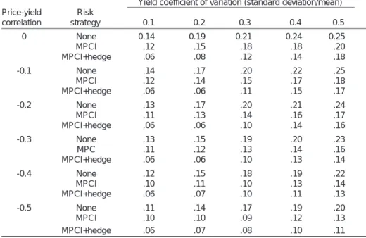
Corn Belt than in bordering areas of production (fig. 5). Thus, the nat-ural hedge is more effective in the Corn Belt, and natural movements in price and yield work to inherent-ly stabilize incomes to a greater extent in that area than elsewhere. In areas outside major producing locations (such as in the Southeast or along the east coast), the natu-ral hedge is much weaker, meaning that low yields and low prices (or conversely, high yields and high prices) are more likely to occur simultaneously. Wheat generally exhibits lower yield-price correla-tions and weaker natural hedges than corn because production is less geographically concentrated. The magnitude of the natural hedge has implications for the effectiveness of various risk-reduc-ing tools. A weaker natural hedge (with a slightly negative correla-tion between price and yield), for example, implies that forward pric-ing by hedgpric-ing in futures or by selling forward on the cash market is more effective in reducing income risk than when a strong natural hedge exists, other factors held constant. In such situations, fixing a sales price for the crop
works to establish one component of revenue, reducing the likelihood of simultaneously low (or high) prices and yields. As a result, hedging corn can, at times, be more effective in reducing risk in those areas outside the major pro-ducing regions of the Corn Belt. Because income risk depends on factors other than the price-yield correlation, however, the effective-ness of hedging in reducing risk is more complicated. In particular, yield variability is an important factor. Corn yields are typically more variable outside the Corn Belt, and hedging effectiveness declines as yield variability in-creases. Because yield variability tends to outweigh the impacts of the price-yield correlation, hedging effectiveness tends to be higher in the Corn Belt than in less robust producing areas. The interaction of yield variability, price variability, and the price-yield correlation in influencing the effectiveness of risk management tools are important factors affecting producers’ choice of the risk management strategies discussed in the next section.
The tendency for corn yields and prices to be negative-ly related is stronger inside than outside the Corn Belt.
Measur
ing P
ric
e and
Y
ield R
isk
Yield-price correlation Less than to -0.40 -0.39 to -0.30 -0.29 to -0.15 Greater than -0.15 Figure 5Farm-level corn yield-price correlation by county, 1974-94
Note: Shaded areas include counties with at least 500 acres planted to corn.
Source: Constructed by ERS from USDA, NASS electronic county yield files, 1997, and USDA, RMA electronic experience and yield record database.
D
Diivveerrssiiffiiccaattiioonn iiss aa ffrreeqquueennttllyy uusseedd rriisskk m
maannaaggeemmeenntt ssttrraatte e--g
gyy tthhaatt iinnvvoollvveess ppa arr--ttiicciippaattiinngg iinn mmoorree tthhaann oonnee aaccttiivviittyy..
T
he price and yield risks dis-cussed earlier, along with a farmer’s attitude toward risk, have a major impact on the choice of risk management strategies and tools. In analyzing the risk-return tradeoffs associated with different approaches, a producer must con-sider his or her expected return to different choices and the variance in returns. Economists have used several approaches to capture these tradeoffs, which vary in how they describe a farmer’s “world view” and how flexible they are in specifying risk attitudes (see appendix 2 for details).E
En
ntte
errp
prriisse
e D
Diiv
ve
errssiiffiicca
attiio
on
n
Diversification is a frequently used risk management strategy that involves participating in more than one activity. The motivation for diversifying is based on the idea that returns from various enterprises do not move up and down in lockstep, so that when one activity has low returns, other activities likely would have higher
returns. A crop farm, for example, may have several productive enter-prises (several different crops or both crops and livestock), or may operate disjoint parcels so that localized weather disasters are less likely to reduce yields for all crops simultaneously.
Many crop farms in the Corn Belt, for example, produce both corn and soybeans. By producing both crops instead of only one, the farm is less at risk of having low revenues because revenues from the two crops are not perfectly positively correlated. In some years, low corn revenues may be counterbalanced by relatively high soybean rev-enues. Diversification in farming has many similarities to the man-agement of financial instruments. Mutual fund managers, for exam-ple, tend to hold many stocks, thus diversifying and limiting the losses of a particular stock doing poorly.
The extent of farm diversification in U.S. agriculture is a difficult concept to measure. USDA analy-sis has measured diversification using an entropy index, which accounts for both the mix of com-modities and the relative impor-tance of each commodity (meas-ured by its estimated value) to
Ho
w
Far
mers Can Manag
e R
isk
H
Ho
ow
w F
Fa
arrm
me
errss C
Ca
an
n M
Ma
an
na
ag
ge
e R
Riissk
k
55Farmers have many options in managing agricultural risks. They can adjust the enterprise mix (diversify) or the finan-cial structure of the farm (the mix of debt and equity capi-tal). In addition, farmers have access to various tools—such as insurance and hedging—that can help reduce their farm-level risks. Indeed, most producers combine the use of many different strategies and tools. Producers must decide on the scale of the operation, the degree of control over resources (including how much to borrow and the number of hours, if any, worked off the farm), the allocation of resources among enterprises, and how much to insure and price forward.
5The ordering of topics in this section does not reflect their relative importance. In addition, the length of discussion associ-ated with a particular topic is not meant to indicate importance, but reflects the com-plexity of the topic and diversity of the literature.
farm businesses (Jinkins). The entropy index spans a continuous range from 0 to 100. The value of the index for a completely special-ized farm producing one commodi-ty is 0. A completely diversified farm with equal shares of each commodity has an entropy index of 100. These entropy indexes for individual producers can be aggre-gated to provide weighted average entropy indexes by farm type, farm size, and other classifications. Based on the Agricultural Resource Management Study (ARMS), USDA’s entropy index work indicates that cotton farms (with an average index of 50) are among the most diversified, pro-ducing substantial quantities of cotton, cash grains, fruits and veg-etables, and in some cases, live-stock (table 3). Poultry farms, where 96 percent of the value of production was from poultry in 1990, were the least diversified, likely in part due to the impor-tance of production contracts. Such contracts can reduce producers’ risk, reducing income variability and lessening producers’ interest in diversification as a risk man-agement tool (Dodson). In the Northern Plains and Corn Belt, farms tended to be less diversified than in other parts of the country, particularly when compared with farms in the Southeast (Jinkins). In addition, data from the ARMS survey indicate that a large por-tion of commercial farming opera-tions specialized in one or two enterprises during the period 1987-91.6On average, one-third of all commercial U.S. farms received
nearly all production from just two enterprises during that period. Further, about one-third of aggre-gate farm production on commer-cial farms was from those engaged in only two enterprises (Dodson). Many factors may contribute to a farmer’s decision to diversify. The underlying theory suggests that farmers are more likely to diversi-fy if they confront greater risks in farming, are relatively risk averse, and face small reductions in expected returns in response to diversification. Other factors may also be important. Continuing the corn and soybean example dis-cussed earlier, planting corn after soybeans may reduce the need for fertilizer because of the nitrogen-fixing properties of soybean plants, and planting both corn and soy-beans may spread out labor and machine use over critical times in the planting and harvesting sea-sons. In situations where livestock is part of the enterprise mix, the operator may be kept busy
throughout the year, and crop and animal byproducts may be used more fully (Beneke).
Depending on the farm’s situation, however, the costs of diversifying may outweigh the benefits, and specializing may be the preferred strategy. Diversifying often
requires specialized equipment (for example, different harvesting attachments), and may be limited by managerial expertise and labor, the productive capacity of the land, and the market potential in the surrounding area (Dodson). Diversifying requires a broader range of management expertise than does producing only one com-modity, and does not typically allow for intensive management. As technologies become more com-plicated, such intensive manage-ment and greater farm specializa-tion may well be increasingly important (Beneke).
Based on USDA research, cotton farms are among the most diversified, while poultry farms are among the most specialized.
Ho
w
Far
mers Can Manag
e R
isk
6Commercial farms in this specific paper were defined as those that received at least $50,000 in annual sales, and where the operator supplied at least 2,000 hours of labor annually and designated farming as his or her primary occupation. This defini-tion is more restrictive than is commonly assumed.
As a result, farmers face tradeoffs when examining diversification as a strategy versus specialization. Specializing can refine the expert-ise needed for a particular produc-tive activity, and may also lead to the economies of scale that lower per unit production costs, increas-ing the profitability of the opera-tion. Indeed, a producer’s decision to specialize (or diversify) may be motivated purely by expected prof-its, with no consideration given to reducing risk. Conversely, the ben-efits associated with diversifying arise through the potential offset-ting revenue interactions among enterprises, and the complemen-tarity of equipment and activities that are used within the farming operation (Scherer).
Empirical analyses of diversifica-tion in farming have usually focused on factors influencing enterprise choices. As an example, a study of over 1,000 crop farms in the San Joaquin Valley of
California examined the relation-ship between diversification and such variables as farm size and wealth. The authors were interest-ed in the tradeoffs between risk reduction and potential size economies in a given activity. They found that wealthier farmers are more specialized, perhaps because they are less risk averse than farmers having lower net worths (Pope and Prescott). Similarly, they
found that corporate farms (with diversified ownership and limited liabilities) are more specialized, as are operators of smaller farms (as measured by cropped acreage) and younger (or less experienced) oper-ators. Young farmers may start small and specialized operations, and perhaps become more diversi-fied as they expand their opera-tions. Farm size (measured by acres cropped) had a positive effect on diversification.
The effects of multiple enterprises on reducing risk have also been analyzed. Schoney, Taylor, and Hayward examined crop enterprise mixes for Saskatchewan farmers, and found that the gross incomes among crops were highly correlat-ed. As a result, they concluded that little risk reduction was gained by diversifying beyond two or three crops. In addition, they found that, although several crops typically had a risk-reducing effect on the portfolio, these benefits were typi-cally outweighed by the lower gross incomes associated with such levels of diversification.
Several diversification studies have also looked at combining live-stock and crop enterprises on an operation, with the results depend-ing on the time period of the analysis and other factors. Held and Zink, for example, found that adding livestock to a hypothetical
The benefits associ-ated with diversify-ing arise through the potential offsetting revenue interactions among enterprises, and the complemen-tarity of equipment and activities that are used within the farming operation.
Ho
w
Far
mers Can Manag
e R
isk
Table 3—Diversification measurement using entropy indexes, 1990
Extent of Value of Average enterprises measure of production from in the Commodity diversification major commodity operation
Entropy
index Percent Number
Cotton 50 62 2.5
Tobacco 42 76 2.2
Cash grains 39 76 1.9
Vegetables, fruits, and nuts 39 80 1.9
Nursery, greenhouse 32 57 1.2
Beef, hogs, and sheep 25 85 1.8
Dairy 24 85 2.4
Poultry 9 96 1.5
Source: Excerpted by ERS from Jinkins, John, “Measuring Farm and Ranch Business Diversity,”Agricultural Income and Finance Situation and Outlook Report, AFO-45, U.S. Dept. Agr., Econ. Res. Serv., May 1992, pp. 28-30.
eastern Wyoming irrigated crop farm could increase gross margin by 7 percent and reduce the coeffi-cient of variation from 0.63 to 0.42. Woolery and Adams indicated that diversified land use, combined with livestock, could increase net income and reduce relative income variability for South Dakota and Wyoming farms. Other studies have reached mixed results as to the risk-return tradeoff (see Persaud and Mapp; Sonka and Patrick). Despite any benefits that may accrue to enterprise diversifi-cation, the opportunities are often limited by resources, climatic con-ditions, market outlets, and other factors (Sonka and Patrick). Geographical diversification (farming at several noncontiguous locations) may also mitigate risks in crop production by reducing the chances that local weather events (such as hail storms) will have a disastrous effect on income. Nartea and Barry examined this form of diversification using Illinois corn and soybean data, and found that risk was not reduced significantly until land parcels were separated by at least 30 miles. They accounted for the costs associated with farming across widely dispersed plots (for example, moving equipment and people and monitoring crop condi-tions), and concluded that widely dispersed tracts typically create unfavorable risk-return tradeoffs for producers. When widely dis-persed parcels are observed, it is likely because of farmers’ desire to expand their operations, and their difficulty in finding additional tracts of farmland that are close to their farming bases. Those most likely to gain from geographic dis-persion of parcels are institutional investors with large acreages who do not have to transport equip-ment and who use tenants to farm their holdings.
V
Ve
errttiicca
all IIn
ntte
eg
grra
attiio
on
n
Vertical integration is one of sever-al strategies that fsever-all within the umbrella of “vertical coordination.” Vertical coordination includes all of the ways that output from one stage of production and distribu-tion is transferred to another stage. Farming has traditionally operated in an open production system, where a commodity is pur-chased from a producer at a mar-ket price determined at the time of purchase. The use of open produc-tion has declined, however, and vertical coordination has increased as consumers have become
increasingly sophisticated and improvements in technology have allowed greater product differenti-ation (Martinez and Reed; Allen). A vertically integrated firm, which retains ownership control of a com-modity across two or more levels of activity, represents one type of ver-tical coordination (Mighell and Jones).7
There are many examples of verti-cal integration in farming. Farmers who raise corn and hay as feed for their dairy operations are vertical-ly integrated across both crop and livestock production. Similarly, cat-tle producers who combine raising a cow-calf herd, backgrounding the animals to medium weights, and feeding cattle to slaughter weights
Opportunities for diversification can be limited by resources, climatic conditions, market outlets, and other factors.
Ho
w
Far
mers Can Manag
e R
isk
7Other types of vertical coordination reflect differing degrees to which a firm at one stage of production exerts control over the quality or quantity of output at other stages (Martinez and Reed). When produc-tion contracts are used, for example, the contractor (or integrator) typically retains control over the commodity and most inputs, and the farmer usually receives an incentive-based fee for production services. In this case, the producer retains little con-trol over production decisions. When mar-keting contracts are used, in contrast, a firm commits to purchasing a commodity from a producer at a price formula estab-lished in advance of the purchase, and the producer retains a large degree of decision-making control. Both production and mar-keting contracts are discussed in subse-quent sections in this report.
are vertically integrated. As these examples illustrate, vertical inte-gration can encompass changing the form of the product (corn into livestock), or combining stages in the production process under own-ership by one entity (as in the cat-tle example).
From the farmer’s perspective, the decision to integrate vertically depends on many complex factors, including the change in profits associated with vertical integra-tion, the risks associated with the quantity and quality of the supply of inputs (or outputs) before and after integration, and other fac-tors. In particular, the relationship between vertical integration and risk involves an evaluation of the expected returns and the variance and covariance of the farmer’s return on investment for the cur-rent activity and the integration alternative (Logan). If the correla-tion is positive and large across activities, the gains in risk effi-ciency from vertical integration may be relatively low. In contrast, a negative correlation across activ-ities implies that integrating verti-cally may well reduce risk for the farmer by internalizing processes within the operation.
In practice, vertical integration in agriculture often involves
owner-ship of both farm production and processing activities, particularly in certain parts of the livestock sector (table 4). Vertical integra-tion is fairly common in the turkey industry, for example, where about 30 percent of production takes place on farms that perform multi-ple functions. On the largest oper-ations, the enterprise mix may include a feed mill, a hatchery, a grow-out operation, a slaughter facility, and a packing plant. In such cases, integration moves both backward into inputs (feed manu-facturing) and forward into the fin-ished, consumer-ready product. Similarly, egg producers with large operations may own their own feed mill, hatchery, laying operation, and freezing/drying plant for the processing of egg products (Manchester).
Vertical integration is also com-mon in certain specialty crops, par-ticularly for fresh vegetable and potato operations (table 4). In these industries, vertical integra-tion often encompasses not only production of the crop, but also sorting, assembling, and packaging products for retail sales. Large, vertically integrated vegetable growers, for example, often both pack and sell their own vegetables, displaying their private brand names on packages, and at times
Vertical integration is much more com-mon in certain live-stock and specialty crop industries than in field crops.
Ho
w
Far
mers Can Manag
e R
isk
Table 4—Extent of farm production coordinated by vertical integration
Commodity 1970 1990 Percent Livestock: Broilers 7 8 Turkeys 12 28 Hogs 1 6
Sheep and lambs 12 28
Field crops: Food grains 1 1 Feed grains 1 1 Specialty crops: Processed vegetables 10 9 Fresh vegetables 30 40 Potatoes 25 40 Citrus 9 8
Other fruits and nuts 20 25
Total farm output 5 8
Source: Martinez, Steve W., and Al Reed, From Farmers to Consumers: Vertical Coordination in the Food Industry, AIB-720, U.S. Dept. Agr., Econ. Res. Serv., June 1996.