Rowan University Rowan University
Rowan Digital Works
Rowan Digital Works
Theses and Dissertations5-18-2020
Prediction of drug-drug interaction potential using machine
Prediction of drug-drug interaction potential using machine
learning approaches
learning approaches
Joseph Scavetta Rowan University
Follow this and additional works at: https://rdw.rowan.edu/etd
Part of the Artificial Intelligence and Robotics Commons, and the Pharmacy and Pharmaceutical Sciences Commons
Let us know how access to this document benefits you -
share your thoughts on our feedback form.
Recommended Citation Recommended Citation
Scavetta, Joseph, "Prediction of drug-drug interaction potential using machine learning approaches" (2020). Theses and Dissertations. 2796.
https://rdw.rowan.edu/etd/2796
This Thesis is brought to you for free and open access by Rowan Digital Works. It has been accepted for inclusion in Theses and Dissertations by an authorized administrator of Rowan Digital Works. For more information, please contact [email protected].
PREDICTION OF DRUG-DRUG INTERACTION POTENTIAL USING MACHINE LEARNING APPROACHES
by Joseph Scavetta
A Thesis
Submitted to the
Department of Computer Science College of Science and Mathematics In partial fulfillment of the requirement
For the degree of
Master of Science in Computer Science at
Rowan University May 1, 2020
Dedications
I dedicate this thesis to my mother, Valerie Scavetta, the hardest working person I have ever known. Through hard times, she has never given up and has always given life her all, inspiring me to do the same. Without her constant support and inspiration, this thesis would not have been possible.
I also dedicate this thesis to Sarah Senula for her love and emotional support. I could not have completed this thesis without her.
iv
Acknowledgments
A special thanks to my committee chair Dr. Serhiy Hnatyshyn for his countless hours of reflecting, reading, encouraging, and most of all his patience throughout the entire process. I thank him for everything that I have learned since joining his research team in 2016. His hard work and dedication towards improving the scientific world has inspired me to further my career and perfect my skills.
Another special thanks to my committee member Dr. Vasil Hnatyshin for all his guidance he has provided me over the years. With his support, I was able to find this team and begin my journey towards this thesis. I thank him for his immeasurable time spent reading and reviewing my work, cultivating my programming skills, and steering me towards the right path.
I also give a special thanks to my committee member Dr. Umashanger Thayasivam for all his support throughout this thesis. I thank him for his ideas and guidance he has provided towards this work.
I extend my thanks towards all the professors who have shaped me from my undergraduate to the completion of my master’s. Though there are too many to list, I would like to give a special thanks to Dr. Svjetlana Vojvodic, Dr. Alison Krufka, Dr. Matthew Travis, Prof. Jack Myers, and Dr. Gabriela Hristescu for the huge impact they have had on my life both academically and personally.
Finally, I want to thank all the scientists from Bristol-Myers Squibb who have advised me on various innovative aspects of drug discovery. A special thanks to Dr. Bruce Car, Dr. Michael Reily, and Dr. Lois Lehman-McKeeman for supporting this research.
v Abstract
Joseph Scavetta
PREDICTION OF DRUG-DRUG INTERACTION POTENTIAL USING MACHINE LEARNING APPROACHES
2019-2020
Serhiy Y. Hnatyshyn, Ph.D. Master of Science in Computer Science
Drug discovery is a long, expensive, and complex, yet crucial process for the benefit of society. Selecting potential drug candidates requires an understanding of how well a compound will perform at its task, and more importantly, how safe the compound will act in patients. A key safety insight is understanding a molecule’s potential for drug-drug interactions. The metabolism of many drug-drugs is mediated by members of the
cytochrome P450 superfamily, notably, the CYP3A4 enzyme. Inhibition of these
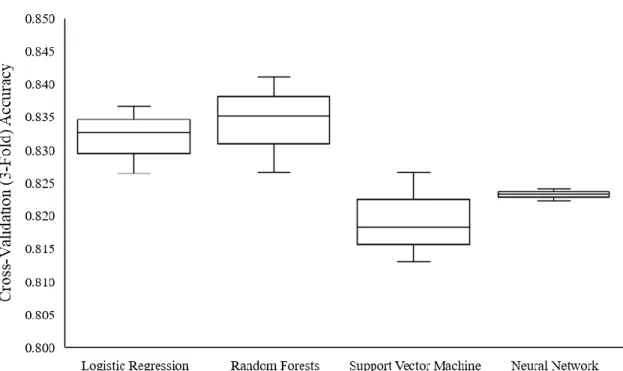
enzymes can alter the bioavailability of other drugs, potentially increasing their levels to toxic amounts. Four models were developed to predict CYP3A4 inhibition: logistic regression, random forests, support vector machine, and neural network. Two novel convolutional approaches were explored for data featurization: SMILES string auto-extraction and 2D structure auto-auto-extraction. The logistic regression model achieved an accuracy of 83.2%, the random forests model, 83.4%, the support vector machine model, 81.9%, and the neural network model, 82.3%. Additionally, the model built with SMILE string extraction had an accuracy of 82.3%, and the model with 2D structure auto-extraction, 76.4%. The advantages of the novel featurization methods are their ability to learn relevant features from compound SMILE strings, eliminating feature engineering. The developed methodologies can be extended towards predicting any structure-activity relationship and fitted for other areas of drug discovery and development.
vi
Table of Contents
Abstract ...v
List of Figures ...ix
List of Tables ...x
Chapter 1: Introduction to Drug Discovery ...1
Drug Discovery Overview ...2
Why Drugs Fail ...4
Drug Candidate Optimization ...5
Rule-Based Drug Discovery ...5
Machine Learning in Drug Discovery ...7
Chapter 2: Machine Learning Overview ...9
Machine Learning Approaches ...10
Linear Models ...10
Decision Trees ...13
Support Vector Machine ...15
Artificial Neural Network ...16
Machine Learning Tools ...18
Data Preprocessing...18
Metrics and Workflows...20
Model Analysis ...22
Predictive Models ...23
Chapter 3: Biological Role of Cytochrome P450 Enzymes...25
vii
Table of Contents (Continued)
Potential for Drug-Drug Interactions ...30
Interferences with the Action of the CYP3A4 Enzyme ...31
Screening for CYP3A4 Inhibitors ...31
Kinetics of CYP3A Meditated Reactions ...32
Bioanalytical Methods to Study CYP3A Mediated Metabolism ...34
In Silico Prediction of CYP–Ligand Interactions ...36
Inhibition Model Review ...36
Chapter 4: Representation, Modeling, and Featurization of Chemical Compounds ...38
Simplified Molecular-Input Line-Entry System (SMILES) ...39
Molecular Fingerprints...41
Molecular Descriptors ...43
Numeric Featurization ...44
Chapter 5: Cytochrome P450 3A4 Inhibitor Modeling ...46
Dataset Curation...47
Inhibitor Models...49
Model Creation ...50
Model Performance and Comparisons ...51
Model Exploration ...53
Novel Machine Learning Approaches ...55
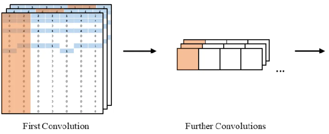
SMILES String Auto-Extraction...57
2D Structure Auto-Extraction ...61
viii
Table of Contents (Continued)
Chapter 6: Conclusions and Future Opportunities ...69
References ...72
Appendix A: Scripts ...80
Appendix B: Data Retrieval ...86
Appendix C: Models ...87
Appendix D: Exploration ...92
ix List of Figures
Figure Page
Figure 1. The standard workflow within the drug development pipeline ...4
Figure 2. The possible outcomes for a binary classification prediction ...21
Figure 3. Ligand-based modeling approaches ...24
Figure 4. Human chromosome 7 with cytogenetic bands displayed ...27
Figure 5. KEGG entry for the CYP3A4 gene ...29
Figure 6. Oxidation reaction catalyzed by CYP3A4. Obtained from KEGG R05727 ....30
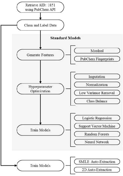
Figure 7. Methodological pipeline used to create predictive models ...47
Figure 8. Cross-validated (3-fold) accuracies for all standard modeling approaches ...52
Figure 9. Most important features for standard modeling approaches ...55
Figure 10. First two layers of the SMILE string auto-extraction architecture ...59
Figure 11. 100x100 pixel matrix displaying Chlorzoxazone and Voriconazole ...62
Figure 12. Cross-validated (3-fold) accuracies for auto-extraction approaches ...63
Figure 13. Inhibition prediction probabilities on FDA inhibitors for all models ...65
Figure 14. SHAP force plots for the best and worst FDA test predictions ...67
x List of Tables
Table Page
Table 1. Known Inhibitors and Inducers for CYP3A4 ...33
Table 2. CYP3A4 Inhibitor Prediction Models in Literature ...37
Table 3.Featurization Methods Useful for Predictive Modeling in Drug Discovery ...39
Table 4. Hyperparameter Optimization for Standard Models ...53
Table 5. SMILE Featurization Matrix for Amifostin ...58
1 Chapter 1
Introduction to Drug Discovery
The origins of contemporary drug discovery can be traced back to the 1800s, when scholars and scientists made many fundamental developments in chemistry: Dmitri Mendeleev published the periodic table, Svante Arrhenius began theorizing about acids and bases, andAugust Kekulé explored aromatic organic molecules, just to name a few [1]. These advances shook the pharmacology field giving birth to a new area of chemistry driven pharmacology. Much later, combinatorial chemistry and high-throughput
screening led to a new paradigm in drug discovery: parsing a plethora of data and compounds to find those that will be successful. However, we can only realize the significance of the findings when we are able to read, extract, and apply the data.
Unfortunately, data analytics in drug discovery was slow to come as shown by the lack of improvement in the number of drugs reaching markets [1].
The next evolution in drug discovery, similar to the establishment of chemistry driven pharmacology, involves an alliance between pharmaceutical disciplines,
bioinformatics, and computer science. Novel developments in computer science research, especially in the area of machine learning, has led to algorithms that allow scientists to use historic data for making predictions on new data, while minimizing cost and the number of errors. Computer aided drug discovery has and will continue to increase the productivity, speed, and efficiency of drug selection and development [2].
2 Drug Discovery Overview
The use of compounds for medicinal purposes has been a vital aspect of human society. Evidence of drug use dates to the prehistoric period, with written evidence appearing in ancient Egypt, China, Rome, Greece, and many other civilizations [3]. In more recent times, pharmaceuticals have increased life expectancy and significantly reduced the effects of disease and sickness. Diseases that had a devastating effects on society in the past, such as bacterial infections, smallpox, and tuberculosis, are now generally non-lethal or have a low-chance to contract [4]. Even diseases that are harder to control or cure, such as cancer or HIV, have recently began to shift from fatal to chronic but manageable [4]. In modern society, quick and efficient drug discovery is becoming more important as the population continues to increase, and people tend to live longer.
Bringing new and improved drugs to the market is important for the health and safety of society. Though much has improved from the birth of pharmaceutical sciences, the lifespan of a drug is still lengthy, and the process is costly. On average, it takes over ten years for a new candidate drug to be approved [5]. Many new candidate compounds never make it to clinical trials due to a prohibitive cost of failure: from 2015 to 2016 the median cost of pivotal clinical trial was estimated at $19 million [6]. Less than 1% of synthesized compounds enter trials [4]. For the drugs that do make it to clinical trials, the probability of success is also low: the highest three success rates were
• 32.6% for ophthalmology drug candidates, • 25.5% for cardiovascular drug candidates, and • 25.2% for infectious disease products;
3
the lowest success rate came in at just 3.4% for oncology trials [7]. Drugs that do succeed through pre-clinical and clinical trials have an average cost of $2.6 billion per compound from start to approval [8]. Many candidate compounds will never result in a new
marketed drug as the candidates will fail, while for those that do succeed, both the duration and costs of the discovery and development are significant.
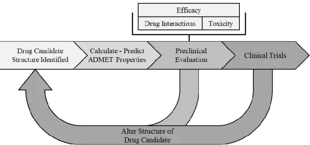
Following Ator et al.’s overview of drug discovery and development, summarized in Figure 1, this process starts with target identification where the receptors that the drug should act upon are selected [4]. Next, the compounds that can act on the target must be found, which often requires high-throughput screening (HTS) and structure-based drug design methods [4]. HTS allows us to select compounds that are active against targets. Compounds from the selection pool are optimized to obtain better drug-like properties [4]. Optimization is focused on careful examination of candidate drug properties such as absorption, distribution, metabolism, excretion, and toxicity (ADMET) [9]. After a drug candidate completes preclinical review and achieves its safety and efficacy goals, it then can enter clinical development. Clinical development consists of four phases:
• Phase I trials test the drug candidate for safety on 10 – 100 healthy human volunteers,
• Phase II trials continue to test safety while also testing efficacy in 50 – 500 of those with the targeted disease,
• Phase III trials test the drug in full-scale with diverse patients and several medical centers, and
4
Figure 1. The standard workflow within the drug development pipeline.
Why Drugs Fail
For a drug to get approved, it must enter and succeed in clinical trials. In Phase I trials most drugs fail due to toxicity. During the Phase II and Phase III trials, drugs often fail due to efficacy problems, although, toxicity still plays a large role in drug failure [10]. Because toxicity and efficacy are the two most common causes of drug failure, ADMET properties are crucial for differentiating between successful drugs and those that will fail.
Failure during the late stages of the clinical trials is not only very costly in terms of money, time, and labor, but it is also potentially dangerous to patients participating in the trials. Clinical trial failures can either be unavoidable due to inadequate scientific advances or could be prevented through scientific rigor, curiosity, and discipline [11]. Unavoidable failures often lack well performing models due to an insufficient knowledge
5
base of the underlying chemistry and/or biology [11]. Preventable failures are explained by a lack of optimal study designs, dosages, and safety data [11]. Overall, learning from earlier mistakes, specifically, collecting, sharing, and analyzing data from both successful and failed drug tests can help reduce the number of avoidable failures. Furthermore, developing new models from these data can also help improve the conditions of the currently unavoidable failures.
Drug Candidate Optimization
The future improvements in the pharmaceutical industry are likely to focus on methods that will significantly reduce failures in clinical trials. Focusing on an early evaluation of new drug candidates will help reduce the associated cost and time of the overall process. Improving pharmacological properties of drug candidates in early stages will reduce the burden on managing compounds that will eventually fail in clinical trials [12]. Selecting successful drug candidates is a complex process that requires an
understanding of drug-like properties, relying on the analyses of overwhelming amounts of data [13]. Various drug candidate selection techniques are discussed below.
Rule-based drug discovery. Rule-based generalizations act as guidelines as to which physiochemical properties one should expect from a successful drug, as compared to a less effective drug candidate. Defining common generalizations for the desired characteristics of drug-like properties is complicated by variations of a drug’s targets and routes of transmission. The Lipinski's rule of 5 is well known approach to determining which properties make a successful drug candidate. This approach specifies upper bounds on molecular properties such as hydrogen bond donors and acceptors, molecular mass,
6
and lipophilicity [14]. While drugs that satisfy Lipinski's rule of 5 are often more successful than those that do not, many exceptions exist where the model would disqualify a successful drug and vice-versa [15]. The Lipinski's ruleset focuses on the absorption properties of a drug, which is only one of many factors that determines a successful drug candidate. Furthermore, this approach is primarily expressive of permeability potential; while solubility and dosage may also play a role in absorption [14]. Also, the bounds apply to oral drugs that do not act as substrates for naturally occurring transporters [14]. While there are limitations to this approach, the Lipinski’s rule of 5 is a useful starting point in selecting important drug-like properties in future drug-prediction models, specifically for absorption models.
Other rule-based methods have been created as an extension to Lipinski's rule of 5 [16]. While the rule-based methods provide a simplified approach for determining drug success, they are limited in substantial ways. Having a strict cutoff points implies that these properties are discrete, rather than continuous [17]. Such assumptions can result in many missed opportunities. Furthermore, these rules are generated only from properties that successful drugs have in common. However, if the property distributions explored in successful drug candidates are similar to failed drug candidates, then these properties are ultimately uninformative [17].
To replace cutoffs with a continuous scale, Bickerton et al. developed the quantitative estimate of drug-likeness (QED) [18]. This approach performs quite well, however, it still does not consider whether a property is truly predictive, i.e. has a different distribution from failed drug candidates. To address both shortcomings of the
7
rule-based approaches, the relative drug likelihood (RDL) can be computed [17]. The RDL approach performs better than QED as it uses distributions from both successful drugs candidates and failed drug candidates. This allows RDL to identify properties that are important to identifying successful drug candidates. Yusof et al. expanded the idea of RDL and created a new algorithm based on the patient rule induction method (PRIM) [19]. PRIM differs from RDL by exploring all the properties simultaneously and identifying redundant properties.
While rule-based methods have improved, they may still lack the ability to generalize non-linear patterns in the data and may miss important relations. Current approaches in drug discovery have now shifted towards applying traditional and novel machine learning algorithms to chemical datasets with a promise of exploring non-linear patterns within data [2].
Machine learning in drug discovery. There have been numerous models and commercial software that can predict various ADMET properties for drug candidates with the help of machine learning techniques [9], [20]. For example, successful drugs typically have a solubility, denoted as log S, with the values ranging from -1 to -5. However, finding the solubility of a compound is difficult. Rather than directly
measuring compound’s solubility, the researchers apply machine learning techniques to construct solubility models using existing data on other compounds. This approach achieves high accuracy of predicting compound solubility, performing as well as experimental measurements [21]. Finding favorable ADMET properties is one of the areas were large sets of data already exist, thus, machine learning can be applied. Other
8
properties, such as a compound’s pharmacokinetics, can also be modeled using machine learning techniques, but experimentally obtained data sets are less common.
Modeling pharmacokinetic properties of a potential drug is important for
predicting success in clinical trials. Pharmacokinetic parameters can be modeled based on the potential drug’s physiochemical properties and through experimental assays [20]. For
example, the random forests, a popular machine learning technique, was used to model the volume of distribution, one of many important pharmacokinetic parameters [20], [22].
Quantitative structure–activity relationship (QSAR) modeling for ligand-based visual screening, has been benefiting from machine learning techniques. Specifically, researchers used machine learning algorithms to determine which drugs match a certain query in a database of potential compounds [23]. QSAR modeling relies on the idea of structural similarity: compounds with similar structures have similar bioactivities [24]. In general, QSAR models employ data from the molecular structure of ligands and
examines physiochemical properties, therapeutic activities, and pharmacokinetic parameters to predict the best molecules for a target [24]. Overall, machine learning based QSAR modeling for visual screening has advanced many aspects of drug discovery and development, specifically, by taking advantage of big data to predict complex
9 Chapter 2
Machine Learning Overview
Simulating human intelligence has been an active area of research in mathematics as far back as the 1700s, when Thomas Bayes developed mathematical fundamentals of what has become Bayes’ Theorem [25]. Machine learning aims to create algorithms that can learn from given data to solve problems without specific instructions. Machine learning is often viewed as a subset of artificial intelligence, though it differs from
common artificial intelligence algorithms in that machine learning emphasizes data rather than pure domain expertise to complete a task. One important sub-section of machine learning is a family of methods that devise models to classify or predict a value for an unknown sample, given a sample of data that has already been classified or has established values. These methods are commonly categorized as supervised machine learning [26].
Supervised machine learning employs statistical methods with fast and efficient algorithms to predict some target function 𝑓: 𝑿 → 𝒚. The target function is unknown, and may always be unknown, however, using some set of input data 𝑥 ∈ℝ𝑑 = 𝑿, and some known output data 𝒚, a function 𝑔 can be created to closely approximate 𝑓. The
combination of input data 𝑿 and output data 𝒚 is called a training set and is denoted as
(𝑥1, 𝑦1), (𝑥2, 𝑦2) … , (𝑥𝑁, 𝑦𝑁). Using the training examples and a set of hypothesis
functions 𝐻, often an infinite set, a learning algorithm can select 𝑔 from 𝐻 that best approximates 𝑓 [27].
10 Machine Learning Approaches
Linear models. Many of the fundamental machine learning algorithms stems from the statistical work of linearly modeling relationships between two or more variables. This type of modeling is often referred to as linear regression, and it was presented as far back as 1886 by geneticist Francis Galton when he was investigating the difference in height between parents and children [28]. The overall goal of linear
regression is to predict some dependent variable 𝑦 given some independent variable(s) 𝑥𝑚 using weighted relationships in the form:
𝑦𝑖 = 𝛽0+ 𝛽1𝑥1+ ⋯ + 𝛽𝑚𝑥𝑚+ 𝜖 Eq. 1
where 𝛽𝑗 acts as corresponding weights of the variable 𝑥𝑗, and 𝜖 is the random error [29].
Using known data for the variable(s) 𝑥𝑚, a prediction of y, denoted as 𝑦̂, can be computed using a modification of equation 1 as follows:
𝑦̂𝑖 = 𝛽0+ 𝛽1𝑥1+ ⋯ + 𝛽𝑚𝑥𝑚 Eq. 2
To find the best predictive function, the weights 𝛽𝑗 can be adjusted to minimize the error
between the predicted 𝑦̂𝑖 and a known 𝑦𝑖. The least squares method is employed to
minimize the error on each known sample 𝒚 = 𝑦𝑖 ∈ℝ𝑛 and the samples’ corresponding prediction from equation 2 [29]. The least squares error can be calculated using the form:
∑ (𝑦𝑖 − 𝑦̂𝑖)2 𝑛
𝑖=1
Eq. 3
There are two common approaches for minimizing the error: (1) using the normal equations for a closed form solution and (2) using an iterative method such as gradient descent. Assuming linear independence between the variables, a unique solution can be found following the closed form:
11
𝜷 = (𝑿𝑇𝑿)−1𝑿𝑇𝒚 Eq. 4
where 𝜷 is an optimal weight vector given a matrix of independent variables 𝑿 = 𝑥𝑖𝑗 ∈
ℝ𝑚×𝑛 and a vector of corresponding dependent variables 𝒚 = 𝑦
𝑖 ∈ℝ𝑛 [27]. A general
solution to the minimization problem is to use gradient descent, which iteratively adjust weights and recomputes the global minimum of the error function, until the best solution is found [30]. Linear regression is a popular statistical method for finding optimal linear relationships between independent and dependent variables. It is often a good starting point for solving a prediction task. However, linear regression has limitations as data can often be non-linear.
A close cousin to linear regression is logistic regression, one of the earliest and most commonly utilized machine learning algorithms for discrete classification [31]. The logistic regression learning algorithm approximates a target function. However, rather than predicting a functional relationship 𝑓(𝑿) = 𝒚, logistic regression models the
probability 𝑃(𝒚|𝑿) of the dependent variables 𝒚 = 𝑦𝑖 ∈ [0,1] belonging to a certain class, given a set of independent variables 𝑿 = 𝑥𝑖𝑗 ∈ℝ𝑚×𝑛 [32]. The base form for
logistic regression is similar to linear regression in equation 1. However, logistic regression applies a soft threshold to equation 1 to achieve the form:
𝑦𝑖 = 𝜃(𝛽0+ 𝛽1𝑥1+ ⋯ + 𝛽𝑚𝑥𝑚+ 𝜖) Eq. 5
where 𝜃 is the logistic function:
𝜃(𝑠) = 𝑒𝑠⁄1 + 𝑒𝑠 Eq. 6
[27]. A common error measure for logistic regression is maximum likelihood, which can be minimized in the form:
12 1 𝑛∑ ln(1 + 𝑒 −𝑦𝑖𝜷𝑇𝒙𝑖) 𝑛 𝑖=1 Eq. 7
Unlike linear regression, logistic regression does not have a closed form solution. Instead, to minimize error, we can employ gradient descent method which can adjust the logistic model towards the steepest decrease in error [33]. Overall, logistic regression is
equivalent to linear regression, aside from the addition of the soft threshold logistic function around the linear model to restrict the functional range to [0,1].
As more variables, or features, are added to linear models, their complexity increases. This can increase the temptation to fit the function too closely to the limited set of data points, or in other words, overfit the training data, which may lead to poor
generalization of new data [34]. To mitigate the effects of overfitting, we can use methods that penalize models for having too large a dependency on any given feature. This method is often called regularization. Regularization adds another term to the error function, which penalizes large weights in the model. The two common methods for
regularization are ridge (L2) and lasso (L1). Ridge regularization adds the term 𝜆 ∑𝑚𝑗=1𝛽𝑗2
to the error function, while lasso regularization adds the term 𝜆 ∑𝑚𝑗=1|𝛽𝑗| [35]. For
example, with lasso regularization equation 7 can be extended to: 1 𝑛∑ ln(1 + 𝑒 −𝑦𝑖𝜷𝑇𝒙𝑖) 𝑛 𝑖=1 + 𝜆 ∑ |𝛽𝑗| 𝑚 𝑗=1 Eq. 8
The 𝜆 acts as a parameter that controls the complexity of the model; i.e., a low 𝜆 allows for a more complicated model while a high 𝜆 reduces the complexity. The differences between the two approaches is that lasso regression allows for the optimal model to drop terms completely (i.e., setting the feature weights to 0), while ridge regularization does
13
not allow a 0 weight [35]. Traditionally, linear models are often the first sought after model as they are fast, efficient, and support regularization methods to avoid overfitting. Though for more complex problems, they may underfit the target function. The field of machine learning also boasts a large number of other algorithms that are not tied to the linear domain, which we will discuss next.
Decision trees. Using a set of criteria or decision points, we can split and classify samples based on the data values. This simple idea is the fundamental concept of decision trees [32]. The decision tree consists of branch nodes that split paths and leaf nodes that act as the outcome for a sample. A decision tree is created from top down; determining which feature of the data will act as the first branch node, and so on. A range of values can be considered for each branch of a feature node. For example, if some value for the feature is less than 10, the tree may branch one way, otherwise, it will branch a separate way. For this reason, ordering features with the most informative features at the top of the tree is crucial. The more information a feature provides, the more likely it will split the data into separable classifications down the tree. Feature importance is determined using one of several feature selection methods.
The first notable feature selection method, introduced by Breiman, Friedman, Stone, and Olshen in 1984, is the Gini index or Gini impurity. The Gini index can be interpreted as the estimated probability of misclassifying a random sample using the selected feature, such that a Gini index of 0 implies a 0% chance that any sample will be misclassified while a Gini index of 1 implies a 100% chance of misclassification [36].
14
Another widely used feature selection method is information gain. Information gain is based on information entropy, which is defined as the average production of novel information from randomly selected data. High entropy relates to a low probability of correctly predicting data, while low entropy relates to a high probability of correctly predicting information [37]. In short, the best feature to select for branching is the one that gains the most information, or in other words, select the feature that results in the greatest reduction of the overall entropy of the prediction task [38].
The strength of decision tree based approaches is accurate classification of data and also determination of the variable importance [32]. Though decision trees can often achieve high accuracy on the training data, they are prone to overfitting. This may lead to a lack of generalization and a decrease in prediction accuracy for new data [39].
Rather than performing classification using only one decision tree, an ensemble of decision trees can be used to significantly increase the performance of the predictive task [40]. Adaptive boosting combines multiple “weak learners” (i.e., models with low
predictive effectiveness) into a single unified strong learner (i.e., a model that performs predictive task well). [41]. Adaptive boosting starts with several decision trees for the dataset, which may be weak learners. Next, the algorithm adjusts the weights of misclassified samples and selects a random set of data to create a new decision tree. Effectively, each new tree is dependent on the errors of the earlier trees. Along with this, each tree stores a weight of importance towards the final collective decision based on how well that individual tree performed.
15
Another popular ensemble method is bootstrap aggregation, or bagging. The bagging method constructs independent decision trees, each created from a bootstrapped sub-sample of the original dataset. This approach does sampling with replacement which allows duplication of observations [40]. The dataset is split into bootstrap samples many times, so that many varying trees are created. The resulting decision trees collectively perform prediction task by selecting the majority answer.
The random forests approach works similarly to the bagging method by creating multiple decision trees, however, created trees differ in their feature sub-space. Each tree is created by sampling the entire training set but with a randomly selected subset of available features [39]. Again, the consensus among individual trees is used to make the final prediction. In practice, the random forests approach relies on a combination of bagging with random feature sub-spacing [42]. Decision trees used collectively as
random forests often provide some of the best average performance and are less sensitive to overfitting as compared to other methodologies [43], [44].
Support vector machine. The support vector machine (SVM) is a versatile machine learning approach that allows classification of linearly separable as well as non-linear data. SVMs are similar to non-linear models, in the sense that they try to fit a line that can split data into two classes. However, the SVM approach has the advantage of finding the optimal hyperplane which maximizes the distance of the data on both sides [45]. This approach allows for more robustness in generalizing towards new data after training, as there is more leeway for the data to trend towards hyperplane without crossing the class boundary. The SMV approach provides model stability by finding the optimal solution
16
every time, yielding consistent results for the same data [45]. This consistency makes support vector machine appealing for practical use. If data is not linearly separable, then the non-linear data can be projected into a high dimension, potentially allowing the data to become linearly separable [45]. SVM’s versatility of handling linear and non-linear data makes it a practical solution to many varying prediction tasks that may differ widely in complexity of the data.
Artificial neural network. Recently, artificial neural networks (ANN) gained popularity and have reached the forefront of machine learning research and technology. Neural networks are based on the perceptron, a fundamental learning algorithm that was modeled from the biological neuron to learn a task [46]. A basic neural network consists of multiple layers of perceptrons, referred to as neurons, which are linked together in numerous ways to produce complex relationships from the input to the output data. Though research on neural networks was stagnant following the criticism of machine learning by Minsky and Papert in their book Perceptrons: an introduction to
computational geometry [47], ANNs returned to the forefront with the creation of back-propagation methods, an increase in computational power, and availability of modern computers. Back-propagation is a technique that allows for the connections, or weights, between one neuron and another to be adjusted towards a global minimization of the output error for many neurons and the true output [48]. Using back-propagation, ANN models consisting of hundreds or more neurons have their connections adjusted in a way that the overall model can take an input and accurately output a response in a short amount of time and with little human effort. The greatest advantage of ANNs is the
17
possibility of modeling complicated non-linear relationships, as neural networks can often find hidden relationships between data that are difficult to detect.
In recent years, many machine-learning practitioners have used the term deep learning to describe a more complex neural networks that have many hidden layers. Deep learning succeeds at modeling even the most complicated relationships than a smaller standard ANN cannot achieve. For example, deep learning allowed computers to learn to play and to defeat professionals at the game of Go [49]. Convolutional neural networks (CNN) and recurrent neural networks (RNN) are examples of deep learning artificial neural networks. Similar to a standard ANN, a CNN has multiple layers of neurons. However, CNNs employ layers of convolution kernels. In contrast to a fully connected ANN that connects all neurons within two adjacent layers, convolution kernels only look at a sub-sample of input neurons to generate an output [50]. Overall, convolutional neural networks work very well with image recognition. The convolution kernels can learn image filters without extensive feature-engineering on the input, and with less computational overhead as compared to a fully connected network.
Recurrent neural networks differ from typical feed-forward networks in creation of connections across neurons based on time or sequence. This adjustment allows for a dynamic learning process where the neural network can remember earlier data in a sequence while training the next step in a sequence. Because of their notion of memory, recurrent networks can work well for sequential inputs such as text or speech [51]. Deep networks have many more variations that are well suited to specific problems.
18 Machine Learning Tools
The data that is being analyzed is often not perfect and may suffer from such deficiencies as missing values, major differences in unit variance, unbalanced classes, or an overwhelming number of features. One must also consider how the models will be evaluated. Although the end goal is to minimize error in the models, the process of determining and comparing errors across models is not resolute. Finally, additional information about models such as the features that were most important or how changes in the features affect the models’ predictions may be of interest.
Data preprocessing. It is uncommon for the data to be collected in a perfect form. Preprocessing is often employed to handle inconsistencies and issues within the collected datasets. There is no simple solution for handling all issues with missing data. Approaches to handle missing data may include removing the samples or features that have missing data or filling in the missing data with some estimated value. If a large portion of data is unavailable, or specific samples or features contain a significant amount of missing data, it may be worth removing samples or features altogether. However, to avoid removing useful data, missing data can be estimated by taking the mean of the feature values, or the mode, if the feature is categorical. Of course, a mixture of both removing and imputing the values can be used as well.
During the data preprocessing phase, the researchers should also consider whether the features should be standardized or normalized. It is possible that one feature may unfairly bias the importance of other features. While in some cases such side effect could be desirable, it is often the result of inconsistent selection of the feature units. This issue
19
is often resolved by normalizing all features to be between 0 and 1 or standardizing the features so that they all have a mean of 0 and a standard deviation of 1.
Another problem that is often ignored is the lack of class balance in the dataset. For example, if a dataset contains 90% of class A samples then the model can be 90% accurate by always predicting that a sample belongs to class A. This issue can be solved by adjusting the accuracy or error metric, but sometimes it is better to address it at the data level instead. There are two main approaches to balancing a dataset: (1) removing from the over-sampled class and (2) adding to the under-sampled class. Removing from the over-sampled class can be as trivial as randomly selecting and removing samples within that class. However, this method risks losing important information from the dataset.
Adding data to an under-sampled class could be achieved by either sampling with replacement or by generating synthetic data points. Sampling with replacement simply duplicates randomly selected samples of under-sampled class. The Synthetic Minority Over-Sampling Technique (SMOTE) is a method for generating synthetic data points. This approach randomly creates samples with features that would exist within the boundaries of the true class data [52].
Sometimes, there are too many features present in a given dataset. An
overabundance of bad features or many correlated features could hurt the performance of a model by allowing it to learn based on misguided data. It can also lead to a significant slowdown of the algorithm. To mitigate the problem of too many features, the
20
(PCA). The univariate feature selection approach selects the 𝑛 best features based on certain statistical test or based on the amount of variance. The advantage to this approach is that the values of the remaining features will not change, those considered
uninformative will simply be removed. However, eliminating features may lead to losing useful information. PCA is more robust against losing information as ittransforms the original features into a few (𝑛) linear combinations of the features (principal
components) with the highest amount of variance [53]. By using orthogonal
transformations, PCA can convert correlated features into linearly uncorrelated principal components. Overall, the intentions of modeling and the amount of redundancy in the dataset may decide which, if any, approaches are taken.
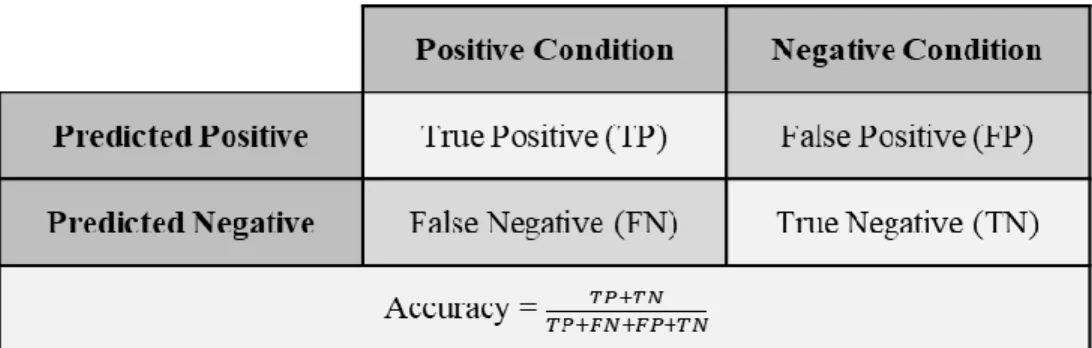
Metrics and workflows. Model accuracy is an important metric for comparison of model performance. Assume that the given dataset consists of two classes: class positive and class negative. In this example, summarized in figure 2, the elements can be classified as follows:
• True positive (𝑇𝑃) - number of positive elements classified as positive, • False negative (𝐹𝑁) - number of positive elements classified as negative, • False Positive (𝐹𝑃) - number of negative elements classified as positive,
and
21
Figure 2. The possible outcomes for a binary classification prediction.
Using the above notation, we can define model accuracy as
(𝑇𝑃 + 𝑇𝑁) (𝑇𝑃 + 𝐹𝑁 + 𝐹𝑃 + 𝑇𝑁⁄ ). The model accuracy specifies the proportion of
predictions that are correct. Other considered evaluation metrics are model’s precision 𝑇𝑃 (𝑇𝑃 + 𝐹𝑃)⁄ , recall 𝑇𝑃 (𝑇𝑃 + 𝐹𝑁)⁄ , false discovery rate 𝐹𝑃 (𝐹𝑃 + 𝑇𝑃)⁄ and/or an F1
score 2𝑇𝑃 (2𝑇𝑃 + 𝐹𝑃 + 𝐹𝑁)⁄ . Model accuracy, along with other metrics, may help truly understand how well a model is performing. For example, the F1 score can be thought of as the harmonic mean of the model’s precision and recall, creating a more robust metric.
The usage of the overall dataset in training and testing models has an important impact on the observed performance metrics. The training and testing models can be viewed as howwell the model is able to train on a given dataset and how well the model is able to classify data it has never seen, respectively. Model bias defines how well the model is trained: a high bias means it did not train well to the dataset and a low bias means it has trained well to the dataset. Model variance explains how well the model performs a classification task: high variance means new data is not classified well and low variance means new data is classified well. To determine model bias, we can simply evaluate the model on the training data. To determine model variance, we must use a
22
dataset that the model was not trained on. To compute model’s bias and variance the dataset could be randomly split into two subsets, creating a training set and a testing set.
The cross-validation approach trains and tests the model while rotating the data in the training and testing set such that all data will be used in the testing set once. Cross-validation is typically considered a better approach as it allows for a statistical
comparison between models and gives a way to find performance anomalies on specific portions of the dataset. Please note that data-preprocessing should be computed only on the testing set and the results should be projected onto the testing set. For example, if missing data is estimated, they should only be estimated using data from the training set, otherwise, information may be leaked into the testing set. Information leaking can bias the scoring functions to overestimate a model’s performance.
Model analysis. After the best performing model is selected, the details of a model’s functionality may be of interest. Some model details that could be useful are the
weighted importance of each variable, or how the different values a variable could obtain influence model predictions. Investigating variable or feature importance is trivial when working with linear based models because the absolute value of the weights associated with the features gives a clear indication as to which features change the prediction more heavily than others. The same is true for decision trees, where the Gini index or the information gain can show how important a feature is within the tree. To understand how a feature’s value influences a model’s sensitivity, partial dependence of various features can be plotted and analyzed. The researchers observe how the output changes across the feature domain when the model is fed the average values of all other features, or one
23
feature value is changed from certain minimum and maximum. The unified framework, SHAP (SHapley Additive exPlanations) assigns each feature an importance value for a given prediction. This is a model agnostic approach for performing exploration
techniques [54], which allow us to better understand the model rather than leaving it a black box.
Predictive Models
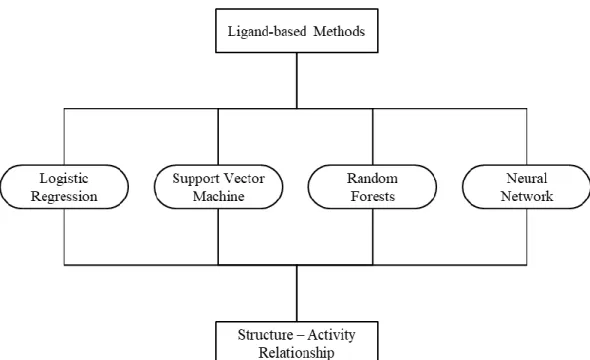
There are many modeling approaches for predicting and evaluating potential drug activities [55]. Using empirical data, one could take a modeling approach that does not rely on fundamental knowledge of the system. This can be reliable as many drug
phenomena are complex and not yet well understood. Two common empirical modeling methods are ligand-based, and target-based approaches [55]. In ligand-based approaches, shown in Figure 3, known active and inactive compounds can be used to detect important structural features for the activity in question. In target-based approaches, the structural features of the enzyme or protein in question can be used to detect potential ligand interactions. Both methods can benefit from machine learning techniques. Target-based approaches can use regression methods to learn and model various enzyme-ligand docking conformations. Ligand-based approaches can use regression or classification techniques to predict a ligand’s activity towards the enzyme or the phenomena being modeled.
24
25 Chapter 3
Biological Role of Cytochrome P450 Enzymes
Cytochromes are an important class of proteins for all biological species.
Containing heme as a cofactor, they are involved in electron transport reactions and act as enzymes in reduction and oxidation reactions. Cytochrome proteins were first discovered in 1884 [56], but didn’t receive the cytochrome name until the 1920s [57]. There are four major types of cytochrome proteins, which can be distinguished by analytical chemistry techniques. Various spectroscopy methods enable analyzing the exact structure of the heme group, analyzing inhibitor sensitivity, and analyzing reduction potential [58]. This chapter focuses on the cytochrome P450 superfamily of enzymes, which named after the characteristic peak formed by absorbance of light at wavelengths near 450 nm, when the heme iron is reduced to carbon monoxide. These enzymes, specifically the 3A4 variant, play an important role in oxidative metabolism and are primarily involved in
steroidogenesis and detoxification [58].
The cytochrome P450 superfamily are categorized as cytochromes that act as monooxygenases, reducing oxygen to a hydroxyl group for incorporation into substrates [59]. Cytochrome P450 enzymes are found in all domains of life and consist of more than 2000 distinct proteins across different species [60]. There has been a total of 57 human genes described within the P450 superfamily with substrates including sterols, fatty acids, eicosanoids, vitamins, and xenobiotics [61]. The oxidation of xenobiotics is particularly important for reducing toxicity that is involved with the incorporation of foreign
26
of drugs, is mediated by P450 enzymes, emphasizing the importance of this family of proteins in drug design [61]. According to their intracellular localization, P450 enzymes may be classified into: 1) microsomal cytochrome P450, which are present mainly in the microsomes of liver cells and represents about 14% of the microsomal fraction of liver cells or 2) mitochondrial cytochrome P450, which are present in mitochondria of many tissues but is particularly abundant in the liver and steroidogenic tissues such as adrenal cortex, testis, ovary, placenta, and kidney.
Metabolic Reactions Mediated by CYP3A
The P450 protein superfamily can be further broken down into families, subfamilies, and finally the specific gene products. The most common and the most versatile member of the cytochrome P450 family of oxidizing enzymes is CYP3A4. Like all other members of this family CYP3A4 is a hemoprotein which is involved in drug metabolism. In humans, the CYP3A4 protein is encoded by the CYP3A4 gene [62]. This gene is part of a cluster of Cytochrome P450 genes and, as visible in Figure 4, is
27
Figure 4. Human chromosome 7 with cytogenetic bands displayed.
According to Wienkers at al [64]the bulk of the metabolism of known drugs in humans is mediated by cytochrome P450 (CYP) enzymes. Among those, the majority of drug oxidations (46%) were carried out by members of the CYP3A family. CYP3A catalyze many reactions involved in drug metabolism as well as in synthesis of
cholesterol, steroids, and other lipids components. Enzymes of CYP3A family mainly found in the liver and in the intestine. Their role is oxidation of small foreign organic molecules (xenobiotics), such as toxins or drugs, so that they can be removed from the body. This makes CYP3A enzymes remarkably important in drug design and
28
The CYP3A subfamily consists of 4 genes: CYP3A4, CYP3A5, CYP3A7, and CYP3A43. Of the four, CYP3A4 tends to have the highest expression and the greatest affinity for metabolizing pharmaceutical drugs [65]. CYP3A4 has a large and flexible active site, and can bind with many large lipophilic compounds, allowing for substrates like immunosuppressants, antibiotics, antidepressants, opioids, and many others [65]. The CYP3A4 protein is an important enzyme in first-pass metabolism, where some amount of a drug may be metabolized before entering systemic circulation [66]. A snapshot of the KEGG entry for CYP3A4 is shown in Figure 5. A sample oxidative reaction catalyzed by CYP3A4 is shown in Figure 6, where a xenobiotic molecule binds with oxygen, creating a less toxic drug and/or a drug that is easier to metabolize downstream.
29
30
Figure 6. Oxidation reaction catalyzed by CYP3A4. Obtained from KEGG R05727.
Potential for Drug-Drug Interactions
The role of metabolic reactions catalyzed by CYPs is to transform the xenobiotic substances to harmless and excretable metabolites [55]. Issues arise in the situation when xenobiotic substances are transformed into a toxic metabolite or the speed of metabolic clearances is significantly altered. The reliance on P450 enzymes to oxidize and facilitate the removal of dugs opens the potential for issues in drug metabolism. Two major issues in drug metabolism are 1) the bioavailability of a drug, i.e., how quickly the drug is metabolized and eliminated, and 2) the accumulation of the drug in the system, which could cause toxic side effects. Issues in bioavailability may arise if the P450 enzymes are induced by another drug, while issues in drug toxicity could occur if the P450 enzymes are inhibited by another drug. The inhibition of P450 enzymes is often the cause of many adverse drug reaction as these drugs are metabolized at slower rates and can begin to accumulate at levels that are toxic [61]. The ability for one drug to affect another drug’s metabolism is referred to as a drug-drug interaction. This interaction is often linked to the inhibition or induction of a P450 enzyme.
31
Interferences with the Action of the CYP3A4 Enzyme
While many drugs are metabolized by CYP3A4 mediated reactions, there are also some drugs which are activated by the enzyme. Some substances, such as grapefruit juice and some drugs, interfere with the action of CYP3A4. These substances will therefore either amplify or weaken the action of the drugs that are modified by CYP3A4,
potentially causing them to exceed the minimum toxicity levels and create adverse side effects. Inhibition can happen in one of three ways, 1) competitive, in which the inhibitor competes with the substrate for the active site within the enzyme, 2) non-competitive, where the inhibitor reduces the activity of the enzyme, and 3) mechanism-based, where the inhibitor is metabolized into a reactive group that can form an irreversible bond with the enzyme. A well reported case of CYP3A4 inhibition was discovered by researchers who noticed an increase in bioavailability of many drugs in patients after consuming grapefruit juice. This effect is due to bergamottin, a furanocoumarin, found within grapefruit that acts as a mechanism-based inhibitor of CYP3A4 [67].
Screening for CYP3A4 Inhibitors
Understanding a drug’s potential to inhibit CYP3A4 is a common step in drug
development; many in vitro and some in vivo assays are conducted on potential drugs to determine if they have any inhibitory ability. The potential for a drug to inhibit CYP3A4 can be assessed in vitro by using a probe substrate. The probe must be a compound that is metabolized by the CYP3A4 enzyme. A commonly used probe is midazolam, a known substrate of CYP3A4, which performs similarly in vitro and in vivo [68]. The screening process works as follows. The probe is placed in a mixture of microsomes that contain
32
the CYP3A4 enzyme and other drugs that are being assessed. If the drug inhibits CYP3A4, the probe can no longer be metabolized at its standard rate. This will result in lower level of metabolites, which can be measured to determine if inhibition was taking place. To increase throughput, CYP3A4 inhibition assays typically use either a
fluorescent probe or Liquid Chromatography Mass Spectrometry (LC-MS/MS) to monitor the rate of probe metabolism [64]. Recently, there has also been an effort in predicting CYP3A4 inhibition in silico, which could save time and resources in the lengthy and expensive drug development pipeline.
Kinetics of CYP3A Meditated Reactions
The kinetics of drug metabolism can be summarized by few computed values: Michaelis-Menten constants (Km), maximal velocities (Vmax), and intrinsic clearance (CLint, Vmax/Km). Similarly, protein inhibition and kinetics can be understood through values such as the inhibition constant (Ki) and the inhibitory concentrations (IC50). While this manuscript focuses on CYP3A4, many compounds that are substrates of CYP3A4 can also be metabolized by CYP3A5 [69]. The speed of metabolism varies by compound and drug class. For example, antifungals on average have a lower CLint than antivirals, with an exception for Itraconazole [69]. The strength of inhibition and induction also varies by compound, a list of compounds with varying degrees of inhibition or induction strength are displayed in Table 1.
33 Table 1
Known Inhibitors and Inducers for CYP3A4
Compound Name Strength Type
Boceprevir Strong Inhibitor Cobicistat Strong Inhibitor Danoprevir and Ritonavir Strong Inhibitor Elvitegravir and Ritonavir Strong Inhibitor Grapefruit Juice Strong Inhibitor Indinavir and Ritonavir Strong Inhibitor Itraconazole Strong Inhibitor Ketoconazole Strong Inhibitor Lopinavir and Ritonavir Strong Inhibitor Posaconazole Strong Inhibitor Ritonavir Strong Inhibitor Saquinavir and Ritonavir Strong Inhibitor Telaprevir Strong Inhibitor Tipranavir and Ritonavir Strong Inhibitor Telithromycin Strong Inhibitor Troleandomycin Strong Inhibitor Voriconazole Strong Inhibitor Clarithromycin Strong Inhibitor Idelalisib Strong Inhibitor Nefazodone Strong Inhibitor Nelfinavir Strong Inhibitor Aprepitant Moderate Inhibitor Ciprofloxacin Moderate Inhibitor Conivaptan Moderate Inhibitor Crizotinib Moderate Inhibitor Cyclosporine Moderate Inhibitor Diltiazem Moderate Inhibitor Dronedarone Moderate Inhibitor Erythromycin Moderate Inhibitor Fluconazole Moderate Inhibitor Fluvoxamine Moderate Inhibitor Imatinib Moderate Inhibitor Tofisopam Moderate Inhibitor Verapamil Moderate Inhibitor Chlorzoxazone Weak Inhibitor Cilostazol Weak Inhibitor Cimetidine Weak Inhibitor Clotrimazole Weak Inhibitor
34 Table 1 (continued)
Compound Name Strength Type
Fosaprepitant Weak Inhibitor Istradefylline Weak Inhibitor Ivacaftor Weak Inhibitor Lomitapide Weak Inhibitor Ranitidine Weak Inhibitor Ranolazine Weak Inhibitor Ticagrelor Weak Inhibitor Apalutamide Strong Inducer Carbamazepine Strong Inducer Enzalutamide Strong Inducer Mitotane Strong Inducer Phenytoin Strong Inducer Rifampin Strong Inducer St. John’s Wort Strong Inducer Bosentan Moderate Inducer Efavirenz Moderate Inducer Etravirine Moderate Inducer Phenobarbital Moderate Inducer Primidone Moderate Inducer Armodafinil Weak Inducer Modafinil Weak Inducer Rufinamide Weak Inducer
Bioanalytical Methods to Study CYP3A Mediated Metabolism
The bioanalytical approaches for metabolism studies can be classified into three main categories: 1) metabolite profiling and identification, which includes
biotransformation and structural analysis both in vitro and in vivo; 2) metabolic stability, which includes profiling the kinetics both in vitro and in vivo, and 3) identification of rate-limiting CYP enzymes in vitro only. The third approach is often used for drug interaction studies which examine the influence of a drug substrate on CYP activity: 1)
35
CYP inhibition: single substrate or cocktail study in microsomes or in hepatocytes, and 2) CYP induction: nuclear receptor activation or cocktail studies in hepatocytes [70]–[74].
Traditional in vitro CYP450 inhibition assays typically target six isoforms of P450: CYP1A2, 2C9, 2C19, 2D6, 3A4, and 3A5, which are known to metabolize more than 90% of drugs. There are two major types of assays: 1) single-substrate assays using known P450 inhibitors and licorice root extract and 2) cocktail assays, also known as N-in-one assays [75].
Single-substrate assay typically evaluates the inhibition of a drug on one P450 isoform at a time. The cocktail inhibition assays can simultaneously evaluate the
inhibition effects of drugs on up to 12 CYP450 isoforms. While cocktail assays are much more efficient than traditional single probe substrate approaches, they still have some disadvantages. They are much more complex and require significant investment into an assay’s parameter optimization. Cocktail assay parameter optimization includes selection
of enzyme protein concentration, minimization of probe substrate interactions,
minimization of solvent effects, complicated detection of probe substrates and usage of a fast and sensitive ultrahigh pressure liquid chromatography (UHPLC) – tandem mass spectrometry (MS/MS) quantitative instrumentation. Typical experimental procedure requires potassium phosphate buffer (100 ml, 0.1 M, pH 7.4) containing 1.3 mM NADPH, 0.2 mg/ml human liver microsomes, and a cocktail of 10 probe substrates including midazolam, which is used for testing CYP3A4 activity [75]. Such experimental procedures are expensive and time-consuming, thus the development of accurate
36 In Silico Prediction of CYP–Ligand Interactions
In silico models to predict characteristics of CYP–ligand interactions attempt to link the structure and properties of ligand with the readouts from CYP mediated
metabolic transformations obtained during in vitro experiments. Such models enable the researchers to exploit experimentally derived data and fill the gaps in understanding of
(1) the affinity of ligand binding to specific CYPs; (2) predicting sites of metabolism;
(3) prediction of inhibition characteristics of test molecules [55]. Inhibition Model Review
The task of predicting CYP3A4 inhibition in silico has been examined before with the help of various theoretical models. A summary of these studies is presented in Table 2. In 2011, Cheng et al. was able to develop a model based on the support vector machine approach, which achieved a cross-validation accuracy of 0.775 [76]. The models utilized MACCS fingerprints determined from the compound structures. In addition, Sun et al. achieved a cross-validation accuracy of 0.811, also using a support vector machine model in 2011. The primary difference between these approaches was in the feature set and the use of custom atom type descriptors [77]. More recently, in 2018, Li et al. used an auto encoder deep neural network that was able to achieve a cross-validation accuracy of 0.850. This study used a set of features generated using the PaDEL software in addition to the compounds’ PubChem fingerprints [78]. In 2019, Wu et al. extended on previous work and developed a new XGBoost approach that achieved a cross-validation accuracy of 0.860 [79].
37 Table 2
CYP3A4 Inhibitor Prediction Models in Literature
Authors Date Model Accuracy # Training Feature Set
Wu et al. 2019 XGBoost 0.860 (3070, 5985) PaDEL1&2D, PubChem FP
Wu et al. 2019 Gradient Boosting DT 0.851 (3070, 5985) PaDEL1&2D, PubChem FP
Wu et al. 2019 Deep NN 0.839 (3070, 5985) PaDEL1&2D, PubChem FP
Wu et al. 2019 Convolutional NN 0.833 (3070, 5985) PaDEL1&2D, PubChem FP
Wu et al. 2019 Random Forests 0.828 (3070, 5985) PaDEL1&2D, PubChem FP
Li et al.. 2018 Multitask AE-DNN 0.850 (3070, 5985) PaDEL1&2D, PubChem FP
Li et al. 2018 Singletask AE-DNN 0.845 (3070, 5985) PaDEL1&2D, PubChem FP
Lee et al. 2017 Laplacian Naïve Bayes 0.799 (1193, 2221) VolSurf+
Su et al. 2015 Support Vector Machine 0.756 (5177, 7456) PaDEL3D, Mold
Su et al. 2015 C5.0 Decision Tree 0.733 (5177, 7456) PaDEL3D, Mold
Sun et al. 2011 Support Vector Machine 0.811 (2334, 4466) Custom Atom types
Cheng et al. 2011 Support Vector Machine 0.775 (4637, 6899) MACCS
Cheng et al. 2011 Stack: SVM; K-NN 0.767 (4637, 6899) MACCS
38 Chapter 4
Representation, Modeling, and Featurization of Chemical Compounds Much of chemical exploration and research relies on computational tools and techniques to represent and study compound structures. However, it is not trivial to efficiently represent a compound in its entirety. At a basic level, we can view a
compound as a graph representing atoms as nodes and bonds as vertices. However, the graph must ensure that the differences in compound configuration are also clearly distinguished. For example, features such as single, double, triple, and ionic bonds, the stereochemistry of an atom, or aromaticity could be difficult to represent. Creating a graph-based representation that covers all of these aspects is not necessarily impossible. In fact, many of these features are often used to visualize compounds [80]. However, existing representations often lack the ability to store structural information or to gather complex information from of a compound in an efficient manner. As summarized in Table 3 there are other techniques that can be used to represent compounds, such as the simplified molecular-input line-entry system (SMILES), generating molecular
fingerprints, or simply using their molecular descriptors. These techniques allow us to describe complex compounds numerically, so that a computer can easily and efficiently process them.
39 Table 3
Featurization Methods Useful for Predictive Modeling in Drug Discovery
Featurization Type Description Ref
SMILE String Alphanumeric characters representing the 2D structure [2] MACCS Fingerprint 960 or 166 structural keys for important substructures [5] PubChem FP Fingerprint 881 structural keys used by the PubChem database [6]
Extended-Connectivity Fingerprint Sets bits based on the structure in a radius of focused atoms [7] PaDEL Descriptor Calculate 797 chemical features including 1D, 2D, and 3D [8] Mordred Descriptor Calculate more than 1800 2D and 3D descriptors [9]
Simplified Molecular-Input Line-Entry System (SMILES)
The simplified molecular-input line-entry system (SMILES) is a widely used representation of compounds. As its name suggests, this method attempts to model a particular compound using a single line of characters. SMILES relies on a set of parsing rules that allow for an unambiguous reconstruction of a compound’s structure. This approach was first introduced in the 1980s [81]. While currently there are other formats, the fundamentals of a SMILE compound representation as a string remain unchanged. For example, atoms are denoted by an uppercase character abbreviation, e.g., carbon is represented as C, nitrogen as N, fluorine as F, chlorine as Cl, etc. Atoms can also be extended to include their charge, as applicable. For instance, a hydroxide may be depicted as [OH-] to indicated that the OH group contains a formal negative charge and a
titanium(IV) atom may be depicted as [Ti+4] to indicate a formal positive charge of 4. To represent bonds, the characters “.”, “-”, “=”, “#”, “$”, “:”, can be used for a non-bond,
40
stereochemistry can be denoted using “/” and “\” characters which represent single bonds connected to a double bonded pair of atoms. For example, F/C=C/F shows the trans configuration while F/C=C\F represents the cis configuration. Often, standard single bonds are assumed and omitted, thus, it is rare to see “-” within a SMILE string.
To store ring structures in a SMILE string, one arbitrary bond within the ring is broken and an integer value is placed instead. At the end of the ring, the integer value is repeated to show that the ring has closed. For example, cyclohexane, a ring of 6 single bonded carbons, would be represented as C1CCCCC1. Integers can be incremented to demonstration additional rings in the compound. Aromatic rings can be shown in a multitude of styles. However, the common syntax is to convert the atom symbols into lowercase characters. For example, using this approach, benzene, a 6-carbon aromatic ring, can be shown as c1ccccc1.
SMILE format also allows representing multiple branching points using parenthesis. Specifically, the atom where the branch starts is followed by the branch portion of the compound surrounded by an open and close parenthesis. For example, isopropyl alcohol is denoted by CC(C)O, indicating that the third carbon branches off of the second and is not bonded to the oxygen. Branch bonds that must be shown, such as a double bond, are denoted within the parentheses. For example, acetone is represented as CC(=O)C to indicate that the oxygen is double bonded to the second carbon, while the third carbon is also bonded to the second carbon rather than the oxygen.
A final consideration in the structural representation of a compound is the chiral configuration of a tetrahedral carbon, where the positional order of the four bonds may be
41
chemically important. There are a several ways to represent chirality. It is often denoted by a clockwise or counter-clockwise bond order with either @ (counter-clockwise) or @@ (clockwise) characters in a SMILE string. For example, the amino acid L-alanine and D-alanine are represented as N[C@@H](C)C(=O)O and N[C@H](C)C(=O)O, respectively.
CANGEN was the first standard algorithm for creating canonical SMILE strings to ensure that each compound has a unique SMILE representation [82]. Recently new algorithms that achieve better results were developed. For example, the public chemical database ChEMBL uses Accelrys's Pipeline Pilot software to generate their canonical SMILE strings [83]. Overall, a standardized canonical SMILE algorithm can ensure uniqueness of compound representation, which is vital when searching for specific compounds, similar compounds, or compounds that contain a particular sub-structure. Canonical SMILE strings can also provide a normalized structure placement when mining structural information from many SMILE strings.
Molecular Fingerprints
Another approach to representing a compound, especially for similarity scoring or for data mining, is molecular fingerprints. The essence of a fingerprint is that the
compound is represented as a variable length string of bits. Each bit identifies the presence or lack of certain piece of information from of the compound. There are many approaches to generating fingerprints, notably, substructure keys-based, topological or path-based, and circular [84].