Trade Credit, Bank Loans, and Monitoring: Evidence from Japan

(1)

C A R F W o r k i n g P a p e r

CARF-F-054

Trade Credit, Bank Loans, and Monitoring:

Evidence from Japan

Yoshiro Miwa University of Tokyo

J. Mark Ramseyer Harvard University

October 2005

CARF is presently supported by Bank of Tokyo-Mitsubishi UFJ, Ltd., Dai-ichi Mutual Life Insurance Company, Meiji Yasuda Life Insurance Company, Mizuho Financial Group, Inc., Nippon Life Insurance Company, Nomura Holdings, Inc. and Sumitomo Mitsui Banking Corporation (in alphabetical order). This financial support enables us to issue CARF Working Papers.

CARF Working Papers can be downloaded without charge from: http://www.carf.e.u-tokyo.ac.jp/workingpaper/index.cgi

Working Papers are a series of manuscripts in their draft form. They are not intended for circulation or distribution except as indicated by the author. For that reason Working Papers may not be reproduced or distributed without the written consent of the author.

(2)

University of Tokyo Faculty of Economics Hongo, Bunkyo-ku, Tokyo miwa@e.u-tokyo.ac.jp Harvard Law School Cambridge, MA 02138 ramseyer@law.harvard.edu FAX: 617-496-6118

Trade Credit, Bank Loans, and Monitoring: Evidence from Japan

By Yoshiro Miwa & J. Mark Ramseyer*

Abstract: Firms in modern developed economies can choose to borrow from

banks or from trade partners. Using first-difference and difference-in-differences regressions on Japanese manufacturing data, we explore the way they make that choice. Whether small or large, they do borrow from their trade partners heavily, and apparently at implicit rates that track the explicit rates banks would charge them. Nonetheless, they do not treat bank loans and trade credit interchangeably. Disproportionately, they borrow from banks when they anticipate needing money for relatively long periods, and turn to trade partners when they face short-term exigencies they did not expect.

This contrast in the term structures of bank loans and trade credit follows from the fundamentally different way bankers and trade partners reduce the default risks they face. Because bankers seldom know their borrowers’ industries first-hand, they rely on guarantees and security interests. Because trade partners know those industries well, they instead monitor their borrowers closely. Because the costs to creating security interests are heavily front-loaded, bankers focus on long-term debt. Because the costs of monitoring debtors are on-going, trade creditors do not. Despite the enormous theoretical literature on bank monitoring, banks apparently monitor very little.

* Professor of Economics at the University of Tokyo, and Mitsubishi Professor of Japanese Legal Studies at Harvard University, respectively. We received helpful suggestions from Douglas Baird, Leslie Hannah, Hidehiko Ichimura, Ronald Mann, Edward Morrison, Hiroshi Ohashi, and Elizabeth Warren, and generous financial assistance from the Center for International Research on the Japanese Economy at the University of Tokyo and the John M. Olin Center for Law, Economics & Business at Harvard University.

(3)

In much of their work on trade credit, scholars focus on when and why we observe it: when do firms tap trade credit and when do they borrow from banks? Why, as Petersen & Rajan (1997: 661) put it, would industrial firms "extend trade credit when more specialized financial institutions such as banks could provide finance"? Under what conditions, as Smith (1992: 674) asked in the Palgrave Dictionary of Money & Finance, would "buyers and sellers prefer trade credit relative to substitutes, such as bank financing, factoring, and cash"?

In modern advanced economies like Japan, firms raise massive amounts through trade credit. Despite the contrary emphases in the literature, they borrow from trade partners when their partners charge less than banks. In turn, those partners tend to charge less when firms need funds for unanticipated exigencies.

Japanese firms primarily turn to banks when they anticipate long-term needs against which they can offer security interests or third-party guarantees. Banks seldom have a comparative advantage in monitoring. As a result, to most borrowers they lend only if the borrower offers that security interest or third-party guarantee. Because the costs of creating these security interests and guarantees are front-loaded, banks tend to lend long-term. By contrast, trade partners do hold a comparative advantage in monitoring, and use it to offer cost-effective (often short-term) loans. At root, trade partners tend to monitor their borrowers closely; banks actually monitor them very little.

With data on the financial practices of both large and small Japanese firms, we first examine the scope of trade credit and bank finance (Section I). We contrast financing patterns over time, across industries, and by firm size. We then estimate the implicit price that trade partners charge their borrowers (Section II). Finally, we use first-difference and first-difference-in-first-differences regressions on 1960s manufacturing data to explore the way firms respond to exogenous shocks (Section III).

I. The Extent of Trade Credit A. Its Scope:

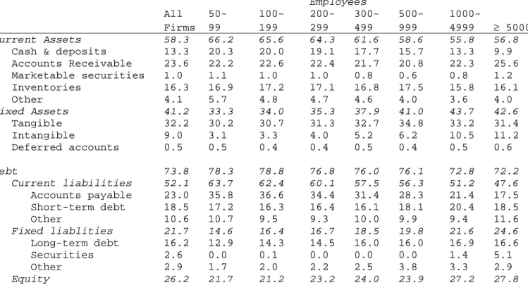
To see how extensively trade creditors fund industrial firms, consider the consolidated balance sheet for manufacturing firms with 50 or more employees (Table 1).1 For this Table 1 and much of the rest of this article, we use Bank of Japan (BOJ) data (described in detail below). From 1961 to 1974, the BOJ surveyed a large number of manufacturing firms -- in 1965, 18,893 firms (a response rate of 74.2 percent).2 To ensure that it reached enough large firms, it did not structure the surveys randomly across firm size. Crucially for our regressions in Section III, however, from each firm it obtained both the figures for that year and the change from the preceding year.

[Insert Table 1 about here.]

For manufacturing firms, the 1960s were years of phenomenal growth. In the five years from 1963 to 1968, Japanese industry grew 90 percent. From 1963 to 1965,

1_{Of the 4,482 firms sampled, 2527 had 50-299 employees, and 1955 had 300 or more employees.}

2_{The BOJ based its survey on a list of all establishments with 50 or more employees produced by the} Ministry of International Trade & Industry for its annual census of manufacturers.

(4)

production at the manufacturing firms grew 22 percent, and from 1965 to 68 another 58 percent. From 1963 to 1968, steel firms grew 117 percent, machinery firms 142 percent, television and radio manufacturers 207 percent, and car companies 372 percent (Tsusho sangyo sho, 1969: 30-11).

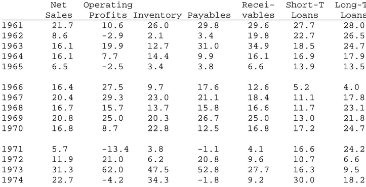
Within these boom times, 1965 was an anomaly: a largely unanticipated and in some sectors deep recession. Manufacturing profits fell over all (Table 2), and in sectors like textile machinery and home electrical goods, production dropped by 20 percent (Tsusho sangyo sho, 1969: 32). The following year was just as anomalous, but in the other direction: a largely unanticipated and sharp recovery. Profits now climbed over 20 percent (Table 2), and in sectors like radio & TV, battery equipment, and petrochemicals, production soared by 40-50 percent (Tsusho sangyo sho, 1969: 32-35).

During these years, Japanese manufacturing firms relied heavily on trade credit. Across all size categories, receivables constituted the largest category of current assets (Table 1; similarly, Petersen & Rajan, 1997; Rajan & Zingales, 1995: 95). And across all but the very largest firms (those with over 5000 employees), payables3 constituted the largest category of current liabilities (Table 1). At all but the biggest companies, firms raised more short-term funds from trade partners than from banks (similarly for U.K. firms, according to the Radcliffe Committee, 1959: 104-05 tab. 18; see also Bank of England, 2003).

In all size categories, firms held 20-25 percent of their assets as receivables (Table 1). Firms of all sizes, in other words, used nearly a quarter of their assets to supply their customers with credit. Trade credit was not something large firms provided the small; it was something both large and small firms provided routinely. Lending was not a business reserved for self-described financial intermediaries; it was an activity to which other firms devoted a large swath of resources.

Over all size categories, payables exceeded inventories. Sometimes they even exceeded inventories by more than 100 percent. Observers occasionally suggest that firms use trade credit to finance their inventories. No doubt they often do. Given how vastly trade credit exceeded inventory, however, they apparently use it for much more.

Nor is this reliance on trade credit new. In related research, we explore the role of trade credit and bank loans in late 19th century Japan. There too, we find that firms relied heavily on their trade partners for funds. There too, manufacturing and trading firms functioned as intermediaries in the financing process (Miwa & Ramseyer, 2005). B. The Effect of Discounting:

Because Japanese sellers heavily discount their notes receivable with banks (or other financial firms), Table 1 (which excludes discounted notes) obscures their status as net creditors.4 According to Table 1, all but the biggest firms hold more payables than receivables. Yet the bigger manufacturing firms (those with 300 or more workers) discounted half their notes (by value) -- from 1961 to 1974, a figure that ranged from 45.3 to 61.7 percent. The smaller firms (those with 50-299 workers) discounted nearly

3_{A substantial fraction of the amounts in "Current liabilities -- other" are also payables. Unfortunately, the} data do not specify that quantity.

4_{Japanese creditors have long maintained an elaborate system for preventing buyers from defaulting on these} notes. The system is described in detail in Ramseyer (1991) and Matsumura & Ryser (1995).

(5)

three quarters -- from 1961 to 1974, 62.5 to 74.1 percent (Nihon ginko, Kibo betsu, various years). Because sellers that discount their notes drop them from their balance sheet, the process arguably disguises the scope of the credit firms provide.

Potentially analogous practices exist elsewhere, of course. In the U.S., trade creditors sometimes sell their receivables to a factor, and an incipient factoring market now operates in Japan as well. In the U.K., firms sometimes purchase credit insurance. Although only the factoring takes the transaction off the balance sheet, both factoring and insurance shift the risk of default to a third party.

By contrast, discounting removes the transaction from the balance sheet but leaves the non-payment risk with the original lender. Although Japanese creditors can use discounting to turn their receivables into cash, as endorser they remain secondarily liable on the notes. In effect, by discounting the notes they post their receivables as collateral for a loan from a bank.

To capture this alternative view of Japanese trade credit, in Table 3 (and the more extensive Table 6, below) we add back discounted notes. In all size categories, manufacturing firms now become net trade creditors. Although receivables exceed payables most strikingly at the biggest firms, even the smallest firms hold substantially more receivables than they owe in payables. Within the manufacturing sector as a whole, firms lend half again as much through trade credit as they borrow.

[Insert Table 3 about here.] C. Industry-Specific Variation:

Firms vary by industry in their lending and borrowing practices. To illustrate the range within manufacturing, in Table 4 we give key values for firms in several prominent industries. Although the firms in all industries were net creditors (receivables/payables > 100), those in machinery lent especially much (receivables/payables). Compared to the amount they borrow from banks, however, they borrowed less from their trade partners than all but the chemical and textile firms (payables/loans).

To explore further the inter-industry variation, for Table 5 we calculate the most popularly used metric: the mean number of days that firms delay before paying their bills. Days Sales Outstanding (DSO) approximates the time a given firm's customers delay in paying their bills, and Days Payables Outstanding (DPO) approximates the time the firm itself stalls. Following much of the literature, we calculate DSO as 365 * (receivables)/(sales). We calculate DPO as 365 * (payables)/(sales). Although some writers divide payables by the cost of goods sold (COGS) rather than sales, we use sales because of both data accessibility and Japanese custom. Because sales will generally exceed COGS (for the firms in the BOJ survey, sales were 98 percent of receipts but COGS was only 82 percent of expenditures; Nihon ginko, Kibo, 1965: 1), this of course lowers the DPO figures.

Here again the larger firms provide more trade credit than the small (Table 5). For its manufacturing-firm survey, the BOJ partitioned firms by workforce size. Unfortunately, for these DSO and DPO figures the Ministry of Finance partitioned firms

(6)

by the more problematic stated-capital.5 Nonetheless, by this measure as well, the bigger firms extend more credit: they let their customers pay more slowly (DSO rises from small firms to large), and pay their own bills more quickly (DPO falls).

Observers sometimes claim that the large trading companies (e.g., C. Itoh & Co., Mitsubishi Corp., Mitsui Trading) finance Japanese manufacturing. Given their large sales base, they do indeed lend massive amounts. Yet wholesaling firms generally offered their customers 60-65 days of credit, while manufacturing firms offered 65-75. The biggest wholesaling firms (the group with C. Itoh, Mitsubishi, and Mitsui Trading) offered 60-75 days, while the largest manufacturers offered 75-85. The wholesaling firms even paid their own bills more slowly: 60-75 days, while manufacturing firms paid in 55-70 (Table 5).

Table 6 confirms several of these generalizations. In virtually every sector except retail sales, firms are net providers of trade credit. Whether in the 1960s or more recently, whether in manufacturing or in the service sector, they lent their trade partners extensive funds.

[Insert Table 6 about here.] II. The Price of Trade Credit A. Introduction:

In asking why firms borrow from their trade partners, scholars typically assume that those partners charge far more than banks. If they charged less, we doubt the Palgrave would ask why buyers preferred their credit. In this, the Palgrave is hardly an outlier. Wilson, Summers & Singleton (1997: 2) describe trade credit as "a premium-priced source of short-term finance." Smith (1992: 674) suggests its rates are "frequently much higher than funds obtained from financial institutions."

Pricing trade credit is hard, of course. Trade partners seldom levy an explicit interest rate, and apparently no central depository collects information on the terms they do impose. As a result, scholars typically obtain a price only by using hypothesized cash-discount terms to "back out" an interest rate.

Petersen-Rajan (1994, 1997) illustrate the practice. At the outset, they assume sellers offer the "2/10 Net 30" terms routinely described in academic accounts. If a buyer pays within 10 days, it can take a 2 percent discount; otherwise, it must pay in full within 30 days. Effectively, a buyer who waits 30 days pays a 2 percent premium for a 20-day loan. Effectively, reason Petersen-Rajan, it borrows at an annual interest rate of over 40 percent.

Like most other writers in the field, Petersen-Rajan (1997: 668; see 1994: 21) take the ubiquity of 2/10 Net 30 on faith. They acknowledge that they "do not know the actual discount offered." They then cite Smith (1987) for the 2/10 Net 30 terms, and use them to calculate the analytically crucial 40+ percent. Smith (1987) herself, though, offers no evidence on the use of 2/10 Net 30. She simply describes the 2 percent discount

5_{The Ministry of Finance also publishes these data in quarterly form, but we here rely on the annual volume} (Okura sho, various years). Note that the figures are the arithmetic mean of the values for the beginning and end of each period. The figures exclude discounted notes. Note that the figures are not noticeably different for the 1960s and 1970s before the purported deregulation of the 1980s. On the insignificance of the earlier regulatory regime, see Miwa & Ramseyer (2004).

(7)

as one of "two most common forms of trade credit" (Smith, 1992: 674). As the other "most common" form, she lists a 30-day loan with no discount at all.

B. Why Take It?

Having concluded that trade credit comes only at an exorbitant price, scholars turn to the obvious conundrum: why take it? Why borrow from a trade partner at 40+ percent when banks lend at less than half the price? To date, the answers come in two variants.

First, scholars suggest that firms take the trade credit when banks will not lend. Because banks ration credit, they write, some firms will have nowhere else to go, and to explain why banks might ration they turn to Stiglitz & Weiss (1981). Given moral hazard and adverse selection, reason Stiglitz-Weiss, in environments with asymmetric information banks may refuse some firms loans at any rate at all.

Within the world at large, continue most scholars, this Stiglitz-Weiss dynamic pushes firms toward trade credit (i) "in countries with less developed financial intermediaries" (Fisman & Love, 2003: 373), and (ii) (an overlapping category) in economies "with undeveloped legal systems that do not effectively support financial development" (Levine, 2004: 38-39). Within the developed economies, it pushes toward trade credit (y) the smaller and newer firms -- "small growing firms" (Wilson, Summers & Singleton, 1997: 2), or (z) firms "that are restricted in their ability to obtain funds" more generally (Schwartz, 1974: 655).

Second, scholars argue that trading partners use the credit (despite its high price) to further "non-financial" goals. Where trade involves substantial relationship-specific investment, for example, perhaps sellers offer credit on terms that let them sort potential buyers by default risk (Smith, 1987). Where buyers can verify product quality only ex post, perhaps they use it to let them verify before paying (Long, Malitz & Ravid, 1993; Lee & Stowe, 1993). Where product demand varies, perhaps buyers and sellers use credit to allocate inventory (Emery, 1987) or precautionary money holdings (Ferris, 1981). And where sellers enjoy market power, perhaps they use credit to enforce price discrimination (Brennan, Miksimovic & Zechner, 1988; Mian & Smith, 1992).

C. Doubts:

1. Cash discounts. -- Despite this literature, scholars offer little actual evidence of usurious credit terms. Although they routinely invoke the canonical 2/10 Net 30, none has measured its prevalence. Certainly, writers in the practitioner press do not focus on 2/10 Net 30. Instead, they typically give a wide range of discount terms.

For example, both the National Association of Credit Management's (2003: 135) Principles of Business Credit and the Credit Research Foundation's (1999: 7) handbook on contractual terms do calculate the implicit interest rates behind cash discounts. Yet rather than focus on any one term, they calculate the effective rates on terms ranging from 0.5/30 Net 90 (3 percent) to 5/15 Net 30 (120 percent). Neither source suggests that 2/10 Net 30 (much less any higher rate) dominates the market.

Within Japan, we know of no evidence that sellers use these extravagant "cash discounts." When we raised the issue with business executives, most refused to believe financially healthy sellers would offer them. If sellers did, they refused to believe

(8)

financially healthy buyers would reject them. Even to offer such a discount, they assured us, would be publicly to admit financial distress.

Indeed, Petersen-Rajan (1994: 24 tab. VII; 1995: 426) themselves find that sellers offer cash discounts -- any cash discounts -- only 30-35 percent of the time. That the sellers offer no discount on 2/3 of their sales does not mean they extend their credit interest-free, of course. It simply means they incorporate the cost of the funds into the price of the goods they sell (or its other attributes). They bundle credit with the goods, in short, and price the resulting package at a rate that maximizes the joint buyer-seller surplus.

2. Stated and effective terms. -- In truth, the true price of credit need not depend on its express terms anyway. As the Arkansas Small Business Development Center (2005) advises its member firms:

Stated terms are irrelevant. ... What the vendor states as terms for payment on the invoice doesn't count. Even finance charges assessed don't count if you never actually have to pay them.

Instead, writes the Center, a firm should pay an invoice five days late to "[s]ee what happens." If nothing does, it should pay the next invoice ten days late. It should continue until the vendor complains, and then "[b]ack off from that point by a few days." Then but only then will it know the seller's "real terms."

In deciding whether to take a cash discount, a rational firm will not calculate the effective interest rate it would bear if it paid the bills by the stated due date. Rather, it will calculate the rate it would bear if it paid by the date it expects the seller actually to enforce. If a supplier states 2/10 net 30 but lets a buyer pay 20 days late, the relevant interest rate is not 40 percent. It is 20.

The terms suppliers actually enforce seem to vary widely by industry, within an industry, and over time. In 2002, for instance, CFO magazine surveyed 967 U.S. companies about (i) how late their buyers paid them (their DSO), and (ii) and how late they paid their own suppliers (their DPO; Reason, 2002). According to its report, the 22 firms in communications technology (with mean sales of $5.4 billion) had a mean DPO of 40 days and a mean DSO of 63. The DPO ranged from 14 to 170, with the group mean down 20 days from the year before; the DSO ranged from 13 to 107, with the group mean down 23 days. The 102 utilities firms ($7.0 billion mean sales) had a mean DPO of 31 days within an 8-148 range, down 14 days from the year before, and a mean DSO of 45 within a 9-639 range, down 14 days.6 And the 62 firms in technology ($7.1 billion mean sales) had a mean DPO of 31 days within a 5-126 range, down 4 days, and a mean DSO of 61 within a 8-178 range, down 10 days.

Although Petersen-Rajan recognize this problem (1994: 21; 1995: 426 n.17), they suggest that firms incur "reputational and pecuniary costs" if they delay. Potentially, of course, dilatory firms do suffer a reputational loss. Sellers may demand trade references from prospective borrowers. They may swap credit information with other sellers. They may buy credit reports from credit-rating firms like D&B and Experian.

Yet precisely because of these potential costs, buyers delay strategically. The Arkansas (2005) small business center, again, advises firms to classify their suppliers by

(9)

precisely these potential costs. If a seller "[s]upplies critical components or materials," it urges them to pay the firm on time. If a seller never charges penalties or notices late payments and sells mass-market goods they could find elsewhere, it tells them to pay the firm late. And -- crucial to the inquiry here -- if a seller "is a member of a professional association or a major supplier in an industry and provides credit information to others," it again advises them to consider any delays costly.

Even the strictest firms sometimes pay late anyway. D&B calls a payment delinquent only if 90 days past due. On a 2/10 Net 30 loan, it thus would mark an account delinquent only after 120 days. It gives a firm a median commercial credit score even if it has "at least 25% of its payments slow and at least 10% of its payments 90 days or more past due." In the U.K., Wilson & Summers (2002) find that firms pay only 60 percent of their bills on time, and typically pay no interest on their delays. According to Table 5, in only rare sectors do Japanese firms pay their bills within 30 days.

3. Comparative monitoring costs.-- For several reasons, many trade creditors should be able to monitor their debtors more cost-effectively than banks, and if they monitor cheaply should be able to lend cheaply as well.7 First, they work either in the same industry as the borrower or in a neighboring one. As a result, they will often hold better information about a borrower’s competitiveness than a bank would ever have. They will know the product it offers, the product its competitors offer, and the level of demand for all those products.

Second, most trade creditors visit a borrower’s facilities regularly to trade. Manufacturers will visit retail outlets that specialize in their goods. They will visit suppliers who offer idiosyncratic products and services. Franchisors will visit their franchisees. Wholesalers may visit retailers that specialize in their goods. If for any of these reasons a creditor already visits a borrower’s facilities, the marginal costs to lending are that much lower.

Third, because a trade creditor maintains regular contact with a borrower’s industry, it can often efficiently collect on any collateral. Should a borrower default, a trade creditor will know where and how to liquidate the assets it obtains. A bank, by contrast, often will not.

If trade creditors can indeed monitor cost-effectively, they should also be able to lend cost-effectively. And if so, then the empirical claim that they lend only at double the interest rate banks charge looks more dubious still. Petersen-Rajan (1995: 426 n.18) suggest that "[t]rade credit is presumably very expensive because firms are not in the business of lending." Yet in bundling loans with the goods they sell, these firms are indeed in the lending business. In competitive credit markets,8 firms that lend only at

7_{One can also contrast the monitoring capabilities of trade partners and banks in terms of economies of scope} that run in differing directions. When trade creditors lend, they use the information they acquire in buying and selling goods and services. When banks lend, they potentially use the information they acquire in taking deposits. Unfortunately for the bank, a firm need not route its transactions through bank accounts. As a result, a bank that handles its accounts necessarily learns only about a potentially incomplete subset of transactions. What is more, the firm can (and most firms do) maintain accounts with multiple banks. Again, its banks will learn about only a subset of its transactions. For both of these reasons, a firm can easily game the system.

8_{Despite the putative regulatory framework, Japanese financial markets have long been competitive. See} generally Miwa & Ramseyer (2004).

(10)

40+ percent will not long stay in business. If firms routinely do offer extensive trade credit, perhaps they do not really lend at 40+ percent.

D. Reexamining Trade Credit:

1. The price on discounted notes. -- To reexamine the price trade creditors charge, we turn to a source other than cash discounts. Rather than rely on terms sellers seldom offer and buyers rarely refuse, we "back out" an implicit interest rate from the note discounting process. Earlier (Section I.B.), we suggested that sellers who discount their notes receivable effectively post them as security for a bank loan. Functionally, however, the process is also equivalent to a loan from a bank to the purchaser with a guarantee from the seller.

Posit three parties: a seller (S), a purchaser (P), and a bank (B). In the quintessential credit sale followed by discounting, (i) S conveys a product to P, (ii) P gives a note promising future payment to S, (iii) S endorses the note and submits it to B, (iv) B pays S a sum of money less than the face amount of the note, and (v) some time later, P pays the face amount of the note to B.

Effectively, this transaction constitutes a loan from B to P, guaranteed by S, under an agreement by P to pay the cash immediately to S. If so, then (a) the difference between the face amount of the note and the cash B pays P (immediately forwarded to S) is the interest on B's loan to P; (b) that interest reflects the risk of a double default by P and S; and (c) the cash paid by P to S represents the sum of (1) the price of the product and (2) the price of S's guarantee.

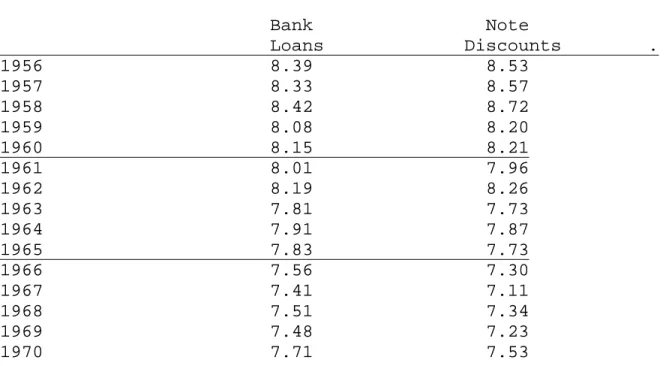
For those receivables that a seller discounts with a bank, then, the discount represents the price of the trade credit to the buyer. As noted earlier, Japanese sellers discount half to three-quarters of their notes. When they do, they obtain rates commensurate with those banks charge on their own loans. Table 7 compares the average annual interest rate firms paid on bank loans from 1956 to 1970, with the effective interest rate they paid on discounted notes. Although they paid less on their loans than on discounted notes in some years, the difference was modest. It never exceeded 3/10ths of a percent, and for nine of the fifteen years they actually paid less on discounts than for loans.

2. The logic to discounted notes. -- In effect, a bank that discounts a note piggy-backs on the trade partner’s (generally) superior monitoring capability. When a seller chooses to offer a buyer credit, it does so because it finds the buyer a cost-effective risk. When that seller endorses the note to a bank, it then credibly vouches for the buyer’s reliability. After all, by endorsing the note it agrees to make good any loss if the buyer defaults. Reasonably enough, banks thereupon willingly discount most notes at low interest rates.

If any selection bias is at work here, it is modest. Sellers do not necessarily discount only their lowest-risk notes. Although they sometimes choose to hold a note rather than discount it, sometimes they choose to do so simply because they do not need more money. If they do not need funds to exploit their competitive projects, they will keep their receivables and collect the funds when they come due.

(11)

Other BOJ data detail the distribution of interest rates on discounted notes and bank loans. Of the 5.9 trillion yen in notes discounted in 1965, banks discounted only 1.3 billion (0.02 percent of the total) at annual interest rates of 10.59 percent or higher. Among the BOJ’s 0.36-percentage-point partitions, the modal rate on discounted notes was 7.69-8.03 percent (900 billion yen, or 15.4 percent of the notes). By contrast, the modal rate on bank loans was 8.40-8.76 percent. In 1970, banks discounted 3.8 billion yen in notes (.03 percent of the total) at 10 percent or higher, and set the modal discount at 8.25-8.50 percent; they made their modal loan at 7.67-8.03 percent. In 1960, they discounted 7.7 billion yen in notes (.29 percent) at 10.59 percent or higher, and set the modal discount at 6.94-7.30 percent; they made their modal loan at exactly the same range (Nihon ginko, Honpo, various years).

3. Trade credit and delegated monitoring. -- Return then to the Palgrave question: why or when would "buyers and sellers prefer trade credit relative to substitutes, such as bank financing"? The evidence on price suggests that for most firms the probable answer is simple: they prefer trade credit when the money they want comes cheaper that way. In corporate finance as in everything else, they equalize on the margin. If extra funds come cheapest from a bank, they take out a loan. If they come cheaper from a trade partner (who may or may not discount its note with a bank), they borrow from that partner instead.

When trade partners do offer a competitive price, they probably do so by exploiting their comparative advantage (discussed above) in screening and monitoring potential borrowers. The logic involved merely extends Diamond's (1984) well-known discussion of delegated monitoring to trade credit. Individuals invest in financial intermediaries, Diamond reasoned, to capture the economies of scale that accrue to screening and monitoring end-users. Rather than screen and monitor directly, they delegate the job to intermediaries. Rather than invest in end-users, they invest in intermediaries who screen and monitor the end-using firms on their behalf.

Although readers sometimes describe Diamond’s model as a theory of banking, by his own terms Diamond offers a theory of financial intermediation more generally. Within that world of intermediaries, banks compete with self-described financial intermediaries like mutual funds and insurance companies. Crucial to the discussion here, they also compete with commercial and industrial firms that offer trade credit.

In effect, Diamond models the intermediary industry as a whole. Sometimes a given financial institution (like a bank) may perform all the functions he describes (raise funds, lend to end-users). Yet often it will not. Instead, a variety of firms may specialize in a variety of the tasks involved in that intermediation. One firm will raise funds from investors. Another will route the funds to the end-users. Rather than invest its funds in end-users itself, a bank may route its funds to a firm better able to screen and monitor them. Rather than perform all the functions Diamond raised, it will split the tasks with an end-user’s trade partners (or the end-user's trade partner's trade partners) instead.

III. The Choice Between Trade Credit and Bank Loans A. Term Structure:

1. Alternative risk-reduction technologies. -- For all the reasons raised earlier, banks will seldom show a comparative advantage in screening and monitoring a borrower.

(12)

That advantage will instead lie with a borrower’s trade partners. Yet that banks cannot monitor as effectively as trade partners does not mean they will not lend. Instead, they will cut their default risk through other strategies. In Japan, they cut it by lending to firms that can offer either security interests or third-party guarantees.

In the fiscal year ending 1960, for instance, banks took security interests on 44.1 percent of their loans (by value), and third-party guarantees on 21.7. In 1965, they took security interests on 45.3 percent and guarantees on 21.6 percent of their loans. And in 1970, they took security interests on 45.7 percent and guarantees on 23.0 (Nihon ginko, Honpo, various years). Although that leaves about a 1/3 of the loans unsecured and without a guarantor, according to the Mitsubishi Bank banks made almost all those loans to a few very large TSE-listed firms. To most borrowers, they lent only if the firm could offer a security interest or guarantee (Mitsubishi, 1983: 76).

The financial services industry is not an industry that harbors many corner solutions. To be sure, firms seldom borrow all their funds from banks. Yet neither do they borrow only from their trade partners. Most firms borrow some funds from their partners and some from banks. Many even borrow from self-described non-bank financial intermediaries. With no legal obligation to do so, they choose to borrow from trade partners, banks, and other intermediaries.9

2. Implications for loan terms. -- These contrasting risk-reduction strategies for banks and trade partners will profoundly affect the term-structure of the loans in place. For expositional simplicity, consider two polar (albeit overlapping) strategies: (A) those designed to prevent a creditor from lending to firms that default, and (B) those designed to protect it if a firm does default. Quintessentially, creditors avoid lending to defaulting firms (Strategy (A)) by monitoring them throughout the course of the loan. If and when a debtor starts to fall into distress, they pull their loans and lend no more.

By contrast, creditors protect themselves in the event of default (Strategy (B)) by demanding security interests. They protect their investment by obtaining the right to take possession and sell specified assets should a debtor not pay. Ideally, they take property worth more than the face amount of the loan. If they do, then whether a debtor defaults or no, they still recover their loan.

These different risk-reduction strategies carry implications for the term structure of the loans involved. To monitor a debtor, creditors must expend resources on an on-going basis. Because even a healthy firm can fall into distress, they will need regularly to devote time and resources to obtaining reliable information about it.

Security interests are different. To obtain a security interest, creditors must invest heavily at the outset, but will incur fewer costs to protect it during the course of the loan. Before they lend, they will require a debtor to post real estate, marketable securities, or other tangible properties. To transform those assets into a legally enforceable security interest, they will draft contracts more complex than a simple loan. They will file those documents with the appropriate government offices. But once they do all this, they have less need (not no need, to be sure) to monitor the debtor on a continuing basis.

9_{As Table 1 shows, firms do not raise all their funds through trade credit and bank loans. Although the two} constitute the largest categories of borrowed money, firms do have a wide variety of ways to adjust to financial shocks: e.g., raise equity, reduce cash and deposits, cut receivables. One cannot simply consider payables and loans as each a "remainder" of the other.

(13)

From their front-end loaded investment, banks and firms will earn quasi-rents so long as the loan remains outstanding. Necessarily, they will have an interest in keeping the arrangement in effect. Conversely, they will find the creation of security interests most cost-effective for those loans which they both expect will stay in place for relatively long periods. When firms have security interests or guarantors that they can cost-effectively offer their creditors, disproportionately they will turn to banks; disproportionately, from them they will borrow long-term.

Because monitoring costs are not front-loaded, creditors earn few quasi-rents from loans that rely on monitoring-based risk-reduction strategies. Rather than invest in legal protections at the outset, the creditors will need regularly to monitor their debtors while the loans remain outstanding. Earning few quasi-rents, they will earn few benefits from keeping the arrangement in place; expecting few quasi-rents, they will have little reason to focus on loans that they expect to stay in place long-term. When firms need loans short-term (or when the costs to a debtor of providing a security interest or guarantor exceed the costs to a creditor of monitoring the debtor), disproportionately the firms will turn to their trade partners.

3. Preliminary observations. -- Figures 1 and 2 reflect this intuition. Here, we chart the year-to-year rate of change in the amount of trade credit and short-term (under 1 year) bank loans over 1961-1974. For informational purposes, we partition the firms by the number of employees.

[Insert Figures 1 and 2 about here.]

The point is simple: the growth rate of bank loans is far steadier than that of trade credit. Although the composition of trade credit and bank loans appears stable over the long-term, it varies considerably over the short-. Firms turn to banks for funds they expect to need for relatively long periods -- unexpected fluctuations in financial need largely do not matter. To cover those fluctuations, they instead turn to their trade partners. Table 8 confirms what the two figures show graphically: the coefficient of variation in the growth rate of trade credit dramatically exceeds the figure for the growth rate of loans. Parenthetically, note that none of this reflects regulatory intervention: the amounts of trade credit and bank loans instead reflect the choices of the lenders and borrowers involved.

[Insert Table 8 about here.] B. Empirical Explorations:

1. Potential misspecification. -- To explore the Palgrave puzzle (when do firms choose trade credit over bank loans), scholars typically regress a firm’s trade credit on its financial and industrial characteristics. Entrepreneurs, however, choose both the boundaries of their firm and its financing decisions partly on the basis of the (unobserved to the scholar) monitoring technology available. 10 For the scholar, this joint determination potentially renders the typical regression misspecified.

In part, the issue raises the make-or-buy (or make-or-sell) question so central to much of industrial organization. Suppose entrepreneur E plans to make gadget G. G includes component C, and in turn becomes part of end-product P. E could buy C on the

10_{Of course, monitoring costs are one type of transactions costs, and monitoring technology is one type of} transaction-cost-saving technology.

(14)

market, assemble G, and then sell it to a P maker on the market. Or he could make C himself. He could incorporate it into G. He could incorporate G into P. He could do all these steps -- integrating vertically from start to finish. And he could even integrate into distribution.

In deciding how far vertically to integrate, E will weigh many issues, but one will involve how cost-effectively he can monitor the production of C and P. In the process, he will also affect the amount of trade credit in circulation. After all, any funds he lends a buyer will constitute trade credit. Any funds he lends an internal division will not. In deciding whether to lend a trade partner funds, E will similarly need to weigh the monitoring technology available. In deciding how much to lend and on what terms, he will again need to consider how cost-effectively he can monitor that partner’s activities.

Necessarily, then, entrepreneur E will choose both (a) the boundaries of his firm and (b) the trade partners to whom he lends on the basis of (c) the monitoring technology available to him. Yet the boundaries of the firm will indirectly affect the amount of trade credit observed. Necessarily, both the usual dependent variable (the financing decision) and independent variables (the firm’s financial and industrial structure) will be jointly determined by an unobserved third measure. Necessarily, any regression of financing measures on firm structure may be misspecified.

2. Differences. -- To address this potential misspecification, we use difference regressions. Consider first the data involved, and then the regression specifications themselves.

(a) Data. Introduction. We base our regressions on the BOJ manufacturing-firm data described earlier. Note that the BOJ did not report firm-level results. Instead, it partitioned the data by industry (14 categories) and firm size (7 ranks, by number of employees) and published the information on the resulting cells. Because several industries lacked firms in the larger ranks, this process yielded slightly fewer than 98 cells.

We do not pool this data across years. After all, by increasing or decreasing its work force, a firm could migrate across cells from year to year. Instead, we rely on the fact that the BOJ asked firms for information both on that year and on the change from the preceding year. By exploiting that change, we calculate differences without pooling the data.

We focus on the three years from 1964 to 1966. As Table 2 shows, the 1960s were generally boom years for Japanese manufacturing firms, and most firms would have anticipated the good performance of 1964. The next year saw a deep recession, however, and 1966 brought a similarly sharp recovery. Many firms would have anticipated neither the 1965 drop nor the 1966 climb.

Variables. We construct the following variables:

Payables: Accounts payable -- kaikake kin plus shiharai tegata. Short-term Loans: bank loans of under one year.

Loans: Total short- and long-term loans. Inventory: Tanaoroshi shisan.

(15)

Sales: Net sales, or jun uriage daka. Income: Operating profits, or eigyo rieki.

Differences. From these variables, we calculate two measures of year-to-year change:

Growth: the percentage growth in a variable. Let Payables be P and Assets be A. Payables (Growth) would equal 100 * (Pt - Pt-1)/Pt-1.

Normalized Change: the change in a variable, normalized by total assets at t-1

and expressed as a percentage. Payables (Normalized Change) would

equal 100 * (Pt - Pt-1)/At-1.

(b) First-differences. We assume that the unobserved determinants of a firm’s basic industrial structure and financing decisions are long-term. Invariant from year to year, they disappear in first-differences. Accordingly, to eliminate the misspecification inherent in the typical regression of financial structure on firm characteristics, we take first-differences.

We first model the composition of firm j’s financial reliance Y (e.g., the amount it raises from trade credit or bank loans) in time t as the product

(1)

Y

t

＝

α

θ

j

S

t

SRV

t

where

α represents the economy-wide determinants of Y (based on the medium- and

long-term expectations of firms in the industry); where θ_j gives the unobserved firm- (or cell-) specific determinants of firm j’s (or cell j’s) reliance on trade credit and bank loans; where

S

t provides a size index; and where SRVt represents the short-run variation

in Y at time t.

In turn, we model St as

S

o

e

gt, where

S

o represents the value of S at t = 0, and g

gives the expected annual growth rate in S. Moreover, we model SRV as the product:

Π

i=1n

(X

it

/X

i0

e

git

)

β_i

The term represents the product of a set of n possible determinants (e.g., inventory, sales, operating profits) of the firm’s reliance on trade credit and bank loans. For each determinant Xi, Xit gives the level actually realized by the firm at time t, and

X

i0

e

git gives

the firm’s expected level at time t as a product of its initial level at t = 0 and

e

g

it (where gi

represents the expected medium- and long-term growth rate of Xi). Equation (1) is thus

equal to:

(2)

Y

t

＝αθ

j

S

o

e

gt

∏

₌ n i 1

(X

it

/X

i0

e

g it

)

βi

Note that

β

_i gives the pace at which the firm’s trade credit or bank loans respond to short-term variations in firm performance. For all the reasons given earlier, we hypothesize that the β_i

'

sfor bank loans will be close to 0, while that for trade credit will be positive.

If we take the logs of Equation (2), differentiate with respect to t, and rearrange the resulting terms, we obtain:

(16)

(3)

it it n 1 i n 1 i i i i t t

X

g

Y

・・

β

∑

= =

+

−

g

Y

₌

This now yields the regression model for our Growth variables. The left term

gives the growth rate in the amount of trade credit or bank loans; the first two terms on the right become a constant; and β_i gives the coefficient on the growth rate of variable Xi. Note that each β will equal the elasticity of the firm’s trade credit or bank loans

with respect to that variable.11

Given the possibility that our specific functional form might be too restrictive, as our second model we use a straightforward first-differences model in which the amount of trade credit or bank loans at each firm (or cell) is a linear combination of several factors. We take first differences, and to avoid heteroskedasticity in the error terms normalize the variables by Assets at time t-1. Because this introduces the effect of Assets in the intercept, we add 1/Assetst-1. as an independent variable in our regressions.

We then use our Normalized Change variables.

We use a variety of proxies for economic activity in our regressions. We posit that firms primarily determine the short-term funds they need by monitoring inventories and sales, and that creditors gauge borrower risk through income levels. We thus use

Inventory, Sales, and Income, and hypothesize that the coefficient on all three will be

(for Payables) positive.

(c) Difference-in-differences. To test whether firms respond differently to anticipated and largely unanticipated shocks,12 we employ a difference-in-differences approach. As noted earlier, we posit that the unobserved determinants of the level of bank loans and trade credit at a firm come in two types: determinants that are constant, and those that vary from year to year. We eliminate the former by differencing the equations -- through first-differences, in other words, all structural and firm-specific factors that are invariant over time disappear.

To test whether firms respond differently to more and less unanticipated exigencies, we add several dummy variables and use a difference-in-differences approach. More specifically, we posit that firms adjust the level of trade credit -- but not of bank loans -- in response to short-term or unanticipated shocks. To test this proposition, we identify several groups of firms that experienced such shocks over 1964-66: the most poorly performing firms during the 1965 recession, and the best performing firms during the 1966 recovery:

Very Low Inventory Growth: all cells that in 1965 had sales growth rates of 5.0

percent or lower (18 percent of the cells).

Low Inventory Growth: all cells that in 1965 had sales growth rates of 6.9

11_{The functional form implies that a regression on the bank loans, with}_β_{=0, will generate a constant term} larger than that on payables. Tables 9-12 give exactly that result.

12_{Although our regressions take the form of classic difference-in-differences regressions, we do not suggest} that the shocks were entirely unanticipated. Instead, for our purposes, we simply posit that firms are better able to predict some financial needs than others -- and use this format to explore whether they adopt different approaches to funding more and less predictable needs. The point of the Table 10 regressions, of course, is that they do indeed adopt different approaches.

(17)

High Inventory Growth: all cells that in 1966 had sales growth rates of 20

percent or higher (29 percent of the cells).

Very High Inventory Growth: all cells that in 1966 had sales growth rates of 25

percent or higher (20 percent of the cells).

Very Low Sales Growth: all cells that in 1965 had sales growth rates of 7.9

Low Sales Growth: all cells that in 1965 had sales growth rates of 10 percent or

lower (30 percent of the cells).

High Sales Growth: all cells that in 1966 had sales growth rates of 20 percent or

higher (33 percent of the cells).

Very High Sales Growth: all cells that in 1966 had sales growth rates of 24

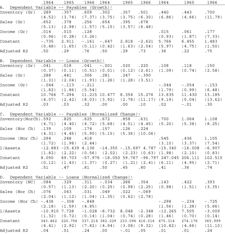
3. Results. -- (a) First differences. In Panel A of Table 9, we use first differences and our Growth variables to explore the determinants of changes in accounts Payable.

The results largely confirm our hypothesis: firms respond to short-term and unanticipated changes by adjusting the amount of money they borrow from their trade partners. Thus, changes in Inventory have a positive, strongly significant, and stable

effect on changes in Payables. Changes in Sales have a similarly positive and significant

effect. Probably because of collinearity, changes in Income have a weaker effect -- but

still significant and positive for 1966. Over the three years, these combinations of

Inventory, Sales, and Income together explain 29 to 75 percent of the variation in

accounts Payable.13

By contrast, firms are far less likely to adjust the amount of their bank Loans

(Panel B). Changes in Inventory, Sales, and Income have only a haphazard effect on

changes in Loans. Most coefficients are insignificant, and when significant the sign of Income is negative: firms respond to increased Income by cutting the amounts they

borrow from banks. Even when significant, the coefficient on Inventory growth (and

hence, the elasticity) is far lower than it is for accounts Payable. All told, the variables

together explain only 0 to 32 percent of the variation in Loans.

In Panels C and D we run similar regressions with our Normalized Change

variables. The results largely track those of our Growth model. Changes in Inventory, Sales and Income have a strong and significant effect on changes in Payables, and

together explain 45 to 81 percent of the variation. They have an only haphazard effect on changes in Loans, and together explain 0 to 24 percent of the variation.

The much smaller effect of changes in firm finances on changes in bank Loans is

not an artifact of pooling short- and long-term loans. In other (unreported) regressions, we run regressions separately on the Growth variables for short-term loans. The

coefficients are significant only for Sales and Income in 1965 and for Income in 1966.

13_{Some of the calculated coefficients are unstable in part because the proxies for economic activity are} occasionally closely correlated. The correlation coefficients between changes in Inventory and in Operating Profits (Normalized Change), for example, were 0.40 in 1966. Between changes in Inventory and in Sales, they were 0.49

(18)

(b) Difference-in-differences. To explore the way firms respond to unanticipated economic shocks in financing their activities, we use a standard difference-in-differences approach. As noted earlier, we identify the firms that experience the shocks with several dichotomous variables based on Sales and Inventory, and use the coefficient on these

variables to capture the effect of the economic shocks. Because changes in Income

explain less of the change in borrowed funds than Sales and Inventory (see Table 9), we

drop the Income variable. Note that we do not demand that the shocks be entirely

unanticipated. Instead, we simply use the regressions to ask whether firms respond differently to more and less unanticipated events.

The resulting Table 10 regressions illustrate several points. First, they confirm the central message of the first-differences regressions in Table 9: firms respond to relatively unanticipated exigencies through trade credit rather than bank loans. Consider the Growth regressions in Panel A. As in first-differences, increases in Inventory and Sales cause firms to borrow significantly more from their trade partners. Panel C

illustrates the same point with the Normalized Change variables. Moreover, changes in Inventory have no effect on bank Loans, and increased Sales actually cause firms to cut

the amount of their Loans (Panels B and D).

Second, those firms for which the recession caused a severe Sales drop in 1965

did cut their Payables more than other firms: the coefficients on Low and Very Low Sales Growth are significantly negative (Panels A.2 and C.2). When interacted with

actual sales levels (VLS * Sales Gr and LS * Sales Gr), the coefficients remain negative

but are no longer uniformly significant. Similar results follow from our regressions with the Inventory shock dummies (though not the interaction terms): the coefficients on Low and Very Low Inventory are again negative (though not statistically significantly

so).14

Third, those firms that experienced dramatic growth in 1966 increased their

Payables more than the others. The High and Very High Sales Growth dummies in the

1966 regressions cause a similar effect (Panels A.3 and C.3): the coefficients are significantly positive, and remain significantly positive when interacted with sales levels (HS * Sales Gr and VHS * Sales Gr).

Last, the exogenous shocks did not affect the Growth in bank Loans (Panels B

and D). In all regressions on Loans, the coefficients on the shock dummies are either

insignificant or in haphazard directions. In 1965, for example, the Inventory and Sales

shock dummies are all insignificant. In 1966, either (a) the coefficients on the Inventory

variable are positive while those on the sales growth dummies are negative, or (b) the coefficients on the Sales variable are negative while those on the inventory growth

dummies are positive.

(c) Pooled data sets. In addition to running the these regressions on the data from the three years separately, for Tables 11 and 12 we pool the data sets and run analogous regressions. Table 11 replicates the first-differences regressions from Table 9, and Table 12 replicates the difference-in-differences regressions from Table 10. The last column on

14_{We bring no priors to the question of whether inventory or sales are more appropriate as continuous and dummy} variables. We include the many permutations to Tables 9-12 only to show that they all generate roughly the same results.

(19)

Table 12 gives the combination of variables that explains a particularly large amount of the variation in the data. Consistently, the results track those from the individual years: firms respond to financial exigencies by adjusting the amounts they borrow from their trade partners; they do not significantly change the amounts they borrow from banks.

[Insert Tables 11 and 12 about here.] IV. Conclusions

Trade credit is not the desperate recourse of the embattled. It is not the safety net for the small. And it is not the province of firms in undeveloped financial markets. Instead, firms both large and small in modern developed economies use trade credit to raise substantial funds.

Neither is trade credit a premium source of funds. Apparently, firms borrow from their trade partners at about the same interest rate (albeit an implicit rate) that banks charge. Apparently, they borrow from their partners when those partners will lend most cheaply. They borrow from banks when their partners will not.

Yet firms do not treat bank loans and trade credit interchangeably. They borrow from banks when they anticipate needing the money for relatively long periods; they turn to trade partners when they face exigencies they did not expect. They do not substantially change the amount of their loans in response to changes in their financial status; they do change the amount of their trade credit in response.

The different term structures of trade credit and bank loans follow from the fundamentally different way trade partners and bankers cut default risk. A trade partner knows his borrower’s industry first hand. To trade, he may even visit his borrower’s business regularly. To reduce his default risk, he monitors his borrower’s activities. Because he incurs his monitoring expenses over time, he willingly lends short-term.

By contrast, although bankers may know how to run a heavily regulated financial intermediary, they know far less about the industries in which their borrowers compete. Banks simply do not have a comparative advantage in monitoring. As a result, to cut their default risk they primarily lend to firms that can offer either third-party guarantees or security interests in property. Because to establish these rights they incur substantial legal expenses at the outset, they lend for relatively long periods.

(20)

References

Arkansas Small Business Development Center. 2005. Managing Accounts Payable. www.asbdc.ualr.edu/bizfacts/1503.asp.

Bais, Bruno & Christian Gollier. 1997. Trade Credit and Credit Rationing. Review of Financial Studies, 10: 903-37.

Bank of England. 2003. Finance for Small Firms -- A Tenth Report. www.bankofengland.co.uk.

Brennan, Michael J., Vojislav Miksimovic & Josef Zechner. 1988. Vendor Financing. Journal of Finance, 43: 1127-41.

Committee on the Working of the Monetary System. 1959. [Radcliffe] Report. London: Her Majesty's Stationery Office.

Credit Research Foundation. 1999. Coming to Terms: The Effect of Terms on Profit and Cash Flow. No Place: Credit Research Foundation.

Diamond, Douglas W. 1984. Financial Intermediation and Delegated Monitoring. Rev. Econ. Stud., 51: 393-414.

Emery, Gary W. 1987. An Optimal Financial Response to Variable Demand. Journal of Financial & Quantitative Analysis, 22: 209-25.

Ferris, J. Stephen. 1981. A Transactions Theory of Trade Credit Use. Quarterly Journal of Economics, 96: 243-70.

Fisman, Raymond & Inessa Love. 2003. Trade Credit, Financial Intermediary Development, and Industry Growth. Journal of Finance, 58: 353-74.

Lee, Yul W. & John D. Stowe. 1993. Product Risk, Asymmetric Information, and Trade Credit. Journal of Financial & Quantitative Analysis, 28: 285-300.

Levine, Ross. 2004. Finance and Growth: Theory and Evidence. NBER Working Paper 10766.

Long, Michael, Ileen B. Malitz & S. Abraham Ravid. 1993. Trade Credit, Quality Guarantees, and Product Marketability. Financial Management, 22: 117-27. Matsumura, Toshihiro & Marc Ryser. 1995. Revelation of Private Information about

Unpaid Notes in the Trade Credit Bill System in Japan. Journal of Legal Studies, 24: 165.

McMillan, Johh & Christopher Woodruff. 1999. Interfirm Relationships and Informal Credit in Vietnam. Quarterly Journal of Economics, 114: 1285-1320.

Mian, Shehzad L., Clifford W. Smith, Jr. 1992. Accounts Receivable Management Policy: Theory and Evidence. Journal of Finance, 47: 169-200.

Mitsubishi ginko. 1983. Kashitsuke keiyaku to ginko torihiki yakutei sho [The Loan Contract and Bank Transactional Contracts]. In Rokuya Suzuki & Akio Takeuchi, eds., Kin'yu torihiki ho taikei [Overview of Financial Transaction Law]. Tokyo: Yuhikaku, pp. 61-85.

(21)

Miwa, Yoshiro & J. Mark Ramseyer. 2004. Directed Credit? The Loan Market in High-Growth Japan. Journal of Economics & Management Strategy, 13: 171.

Miwa, Yoshiro & J. Mark Ramseyer. 2005. Japanese Industrial Finance at the Close of the 19th Century: Trade Credit and Financial Intermediation, Explorations in Economic History, __:__ (2005).

National Association of Credit Management. 2003. Principles of Business Credit, Field Version 4. Columbia, MD: National Association of Credit Management.

Nb, Chee K., Janet Kiholm Smith & Richard Smith. 1999. Evidence on the Determinants of Credit Terms Used in Interfirm Trade. Journal of Finance, 54: 1109-29.

Nihon ginko. Various years. Kibo betsu kigyo keiei bunseki [Analysis of Firm Management, by Firm Size]. Tokyo: Nihon ginko.

Nihon ginko. Various years. Honpo keizai tokei [Economic Statistics of Japan]. Tokyo: Nihon ginko tokei kyoku.

Okura sho. Various years. Hojin kigyo tokei nempo [Annual Statistics on Corporations]. Tokyo: Okura sho.

Petersen, Mitchell A., & Raghuram G. Rajan. 1994. The Benefits of Lending Relationships: Evidence from Small Business Data. Journal of Finance, 49: 3-37. Petersen, Mitchell A., & Raghuram G. Rajan. 1995. The Effect of Credit Market

Competition on Lending Relationships. Quarterly Journal of Economics, 110: 407-43.

Petersen, Mitchell A., & Raghuram G. Rajan. 1997. Trade Credit: Theories and Evidence. Review of Financial Studies, 10: 661-91.

Rajan, Raghuram G., & Luigi Zingales. 2003. Saving Capitalism from the Capitalists: Unleashing the Power of Financial Markets to Create Wealth and Spread Opportunity. New York: Crown Business.

Ramseyer, J. Mark. 1991. Legal Rules in Repeated Deals: Banking in the Shadow of Defection in Japan. Journal of Legal Studies, 20: 91.

Reason, Tim. 2002. We Can Work It Out: The 2002 Working Capital Survey. CFO Magazine. August, 2002.

Schwartz, Robert A. 1974. An Economic Model of Trade Credit. Journal of Financial & Quantitative Analysis, 9: 643-57.

Smith, Janet Kilholm. 1987. Trade Credit and Informational Asymmetry. Journal of Finance. 42: 863-72.

Smith, Janet Kilholm. 1992. Trade Credit. In Peter Newman, Murray Milgate & John Eatwell, eds. The New Palgrave Dictionary of Money & Finance. London: Macmillan, pp. 673-75.

Tsusho sangyo sho. 1969. Ko kogyo shisu nempo [Annual Index of Mining and Manufacturing]. Tokyo: Tsusho sangyo sho.

(22)

Wilner, Benjamin S. 2000. The Exploitation of Relationships in Financial Distress: The Case of Trade Credit. Journal of Finance, 55: 153-78.

Wilson, Nicholas, Barbara Summers & Carole Singleton. 1997. Small Business Demand for Trade Credit, Credit Rationing and the Late Payment of Commercial Debt: An Empirical Study. Unpublished.

(23)

Table 1: 1964 Balance Sheets (%), by Firm Size

Employees

All 50- 100- 200- 300- 500- 1000-

Firms 99 199 299 499 999 4999 ≥ 5000

Current Assets 58.3 66.2 65.6 64.3 61.6 58.6 55.8 56.8

Cash & deposits 13.3 20.3 20.0 19.1 17.7 15.7 13.3 9.9

Accounts Receivable 23.6 22.2 22.6 22.4 21.7 20.8 22.3 25.6 Marketable securities 1.0 1.1 1.0 1.0 0.8 0.6 0.8 1.2 Inventories 16.3 16.9 17.2 17.1 16.8 17.5 15.8 16.1 Other 4.1 5.7 4.8 4.7 4.6 4.0 3.6 4.0 Fixed Assets 41.2 33.3 34.0 35.3 37.9 41.0 43.7 42.6 Tangible 32.2 30.2 30.7 31.3 32.7 34.8 33.2 31.4 Intangible 9.0 3.1 3.3 4.0 5.2 6.2 10.5 11.2 Deferred accounts 0.5 0.5 0.4 0.4 0.5 0.4 0.5 0.6 Debt 73.8 78.3 78.8 76.8 76.0 76.1 72.8 72.2 Current liabilities 52.1 63.7 62.4 60.1 57.5 56.3 51.2 47.6 Accounts payable 23.0 35.8 36.6 34.4 31.4 28.3 21.4 17.5 Short-term debt 18.5 17.2 16.3 16.4 16.1 18.1 20.4 18.5 Other 10.6 10.7 9.5 9.3 10.0 9.9 9.4 11.6 Fixed liablities 21.7 14.6 16.4 16.7 18.5 19.8 21.6 24.6 Long-term debt 16.2 12.9 14.3 14.5 16.0 16.0 16.9 16.6 Securities 2.6 0.0 0.1 0.0 0.0 0.0 1.4 5.1 Other 2.9 1.7 2.0 2.2 2.5 3.8 3.3 2.9 Equity 26.2 21.7 21.2 23.2 24.0 23.9 27.2 27.8

Note: Manufacturing firms only. Sample construction described in text.

Source: Nihon ginko, Kibo betsu kigyo keiei bunseki [Analysis of Firm Management, by Firm Size] (Tokyo: Nihon ginko, 1965) (fiscal year 1964).

(24)

Table 2: Growth Rates (%) of Selected Financial Variables

Net Operating Recei- Short-T Long-T

Sales Profits Inventory Payables vables Loans Loans

1961 21.7 10.6 26.0 29.8 29.6 27.7 28.0 1962 8.6 -2.9 2.1 3.4 19.8 22.7 26.5 1963 16.1 19.9 12.7 31.0 34.9 18.5 24.7 1964 16.1 7.7 14.4 9.9 16.1 16.9 17.9 1965 6.5 -2.5 3.4 3.8 6.6 13.9 13.5 1966 16.4 27.5 9.7 17.6 12.6 5.2 4.0 1967 20.4 29.3 23.0 21.1 18.4 11.1 17.8 1968 16.7 15.7 13.7 15.8 16.6 11.7 23.1 1969 20.8 25.0 20.3 26.7 25.0 13.0 21.8 1970 16.8 8.7 22.8 12.5 16.8 17.2 24.7 1971 5.7 -13.4 3.8 -1.1 4.1 16.6 24.2 1972 11.9 21.0 6.2 20.8 9.6 10.7 6.6 1973 31.3 62.0 47.5 52.8 27.7 16.3 9.5 1974 22.7 -4.2 34.3 -1.8 9.2 30.0 18.2

Notes: Manufacturing firms with 50 or more employees. Trade credit excludes notes. Sample construction described in text. Source: see Table 1 (various years).

- - -

Table 3: 1964 Accounts-Payable and Accounts-Receivable, by Firm Size (%) Employees All 50- 100- 200- 300- 500- 1000- Firms 99 199 299 499 999 4999 ≥ 5000 Receivables/Payables 154.7 128.7 123.4 128.1 128.6 129.1 156.8 186.6 Receivables/Sales 36.1 27.5 30.1 31.9 33.3 31.6 36.8 42.1 Payables/Sales 23.3 21.4 24.4 24.9 35.9 24.5 23.5 22.5

Notes: Receivables include notes discounted with banks;

receivables in Table 1 exclude discounted notes. Manufacturing firms only. Sample construction described in text.

(25)

Table 4: Trade Credit in Selected Industries, 1964-66 Averages, by Firm Size (%)

Employees

50- 100- 200- 300- 500- 1000-

99 199 299 499 999 4999 ≥5000

A. Discounted Notes/All Notes

Textiles 78.5 77.0 76.4 72.0 77.6 65.8 49.7

Chemicals 63.4 62.8 61.3 64.3 64.0 53.7 55.5

Iron & Non-Ferr. Metals 72.6 75.7 75.4 74.6 75.8 70.1 60.2

Machinery 70.1 71.1 57.8 53.6 53.6 46.6 27.8 Electrical Equipment 78.8 73.4 73.6 74.5 74.5 54.6 40.5 Transportation Equip. 67.8 62.7 63.4 52.7 52.7 41.8 19.6 B. Receivables (A)/Sales Textiles 29.3 27.9 29.9 27.0 28.0 30.0 30.0 Chemicals 33.2 36/8 39.1 37.7 37.5 40.6 42.1

Machinery 36.3 40.8 45.0 46.5 52.3 52.7 65.2 Electrical Equipment 29.3 29.2 29.1 30.5 34.1 41.5 46.6 Transportation Equip. 29.1 31.0 30.6 33.0 39.7 41.5 56.3 C. Receivables (B)/Sales Textiles 10.9 11.6 11.8 12.4 11.5 15.6 18.7 Chemicals 18.1 20.6 21.6 20.6 21.3 25.2 26.9

Machinery 18.6 21.4 27.7 29.9 35.2 39.2 55.7 Electrical Equipment 15.3 17.3 17.6 17.7 20.7 30.1 38.0 Transportation Equip. 17.4 18.5 18.9 22.7 27.3 32.5 51.4 D. Payables/Sales Textiles 21.9 21.9 23.5 22.8 22.6 22.7 19.1 Chemicals 36.5 28.3 26.4 25.8 25.8 26.4 27.3

Machinery 25.4 28.3 28.1 28.8 30.5 27.2 27.1 Electrical Equipment 22.2 24.4 26.9 26.1 27.4 27.9 21.3 Transportation Equip. 23.9 28.2 31.3 36.5 36.0 30.6 24.4 E. Receivables (A)/Payables Textiles 133.5 127.6 127.5 118.3 124.0 132.3 157.0 Chemicals 112.9 130.1 147.9 146.5 146.3 154.4 154.8

Machinery 143.2 144.3 160.7 161.8 172.1 194.5 240.5 Electrical Equipment 132.1 119.9 108.4 117.2 124.5 148.8 218.8 Transportation Equip. 123.6 113.6 101.2 105.1 118.3 140.1 234.8 F. Receivables (B)/Payables Textiles 49.5 53.0 50.3 54.5 51.0 69.0 97.8 Chemicals 60.6 73.0 81.7 80.0 83.0 95.9 98.7

Machinery 73.4 75.9 98.6 104.1 115.8 144.9 205.5

Electrical Equipment 69.4 70.9 65.6 68.0 75.7 108.1 178.4

Transportation Equip. 73.1 67.4 61.6 71.4 80.0 109.5 213.6

(26)

Table 4 (Cont'd) Employees 50- 100- 200- 300- 500- 1000- 99 199 299 499 999 4999 ≥5000 G. Payables/Loans Textiles 127.3 90.3 85.5 86.6 68.7 62.4 54.0 Chemicals 146.5 129.4 128.1 99.5 72.0 52.3 45.3

Machinery 100.9 110.9 81.6 79.4 81.9 63.7 69.9 Electrical Equipment 140.6 139.8 150.3 151.4 128.7 88.0 53.9 Transportation Equip. 110.3 143.4 151.3 172.9 124.6 87.0 47.0 H. Inventories/Payables Textiles 62.2 67.9 64.7 60.1 79.6 94.5 114.0 Chemicals 36.1 42.9 45.7 53.9 55.9 50.5 57.9

Machinery 45.3 52.4 61.4 72.0 76.7 82.1 74.4

Electrical Equipment 42.2 51.7 49.3 55.8 60.8 82.9 108.4

Transportation Equip. 36.9 33.4 39.3 40.6 45.1 64.3 89.8

Notes: Receivables (A) include notes discounted with banks. Receivables (B) exclude discounted notes. Sample construction described in text.