Global asset pricing

(1)

Federal Reserve Bank of Dallas

Globalization and Monetary Policy Institute

Working Paper No. 88

Global Asset Pricing

*

Karen K. Lewis

University of Pennsylvania

August 2011

Abstract

Financial markets have become increasingly global in recent decades, yet the pricing of

internationally traded assets continues to depend strongly upon local risk factors, leading to

several observations that are difficult to explain with standard frameworks. Equity returns

depend upon both domestic and global risk factors. Further, local investors tend to

overweight their asset portfolios in local equity. The stock prices of firms that begin to trade

across borders increase in response to this information. Foreign exchange markets also

display anomalous relationships. The forward rate predicts the wrong sign of future

movements in the exchange rate, implying that traders can make profits by borrowing in

lower interest rate currencies and investing in higher interest rate currencies. Furthermore,

the sign of the foreign exchange premium changes over time, a fact difficult to reconcile

with consumption variability. In this review, I describe the implications of the current body

of research for addressing these and other global asset pricing challenges.

JEL codes: G11,G12,G13,G14,G15

*

Karen K. Lewis, Department of Finance, Wharton School, 2300 SHDH, University of Pennsylvania,

Philadelphia, PA 19104-6367. This paper was prepared for

the Annual Review of Financial Economics, DOI: 10.1146/annurev-financial-102710-144841. All opinions expressed in this review are mine alone. Nevertheless, I am grateful for comments from a number of people including Markus Brunnermeier, Choong Tze Chua, Max Croce, Bernard Dumas, Cam Harvey, Bob Hodrick, Andrew Karolyi, Sandy Lai, Edith Liu, Emilio Osambela, Lasse Pedersen, Nick Roussanov, and Frank Warnock. The views in this paper are those of the author and do not necessarily reflect the views of the Federal Reserve Bank of Dallas or the Federal Reserve System.

(2)

1 Introduction

Financial markets have become increasingly global in recent decades. Indeed, the recent …nancial crisis highlighted the strong interlinkages among global capital markets. Therefore, the casual ob-server might logically presume that internationally traded assets are globally priced. Nevertheless, the body of international …nancial research shows that prices of globally traded assets depend upon local country-speci…c risks. While the importance of these local factors may be diminishing over time, studies continue to point to the signi…cance of both global and local e¤ects.

What are the country-speci…c e¤ects that matter in a global …nancial market? These fac-tors naturally surround di¤erences in capital markets that are inherently national. First, many countries maintain their own monetary policy. Therefore, asset prices across countries often in-corporate aspects of currency risk. Moreover, these di¤erences in aggregate price policy can a¤ect asset pricing relationships in models without money through real exchange rate changes. Second, countries often di¤er in the openness of the capital markets. These di¤erences can either be ex-plicit as in the case of a government policy to restrict capital movements. Or they can arise in more subtle forms due to higher informational costs to foreigners. Collectively, these di¤erences are often called segmented capital markets. Finally, countries di¤er through government …scal policy, a¤ecting returns in various ways. For example, the government may tax returns directly or increase the perceived risk of future taxes. Alternatively, the government’s …scal behavior may generate perceived sovereign risk that impacts the returns of all securities from that country.

While monetary policy, …scal policy, and segmented markets identify convenient groupings of factors a¤ecting international asset pricing, they are by no means mutually exclusive. For example, international investors may perceive greater sovereign risk in a country with a large …scal de…cit and that country may also have more segmented capital markets.

(4)

relation-ships leads to several observations that are di¢ cult to explain with standard models. For example, equity returns depend upon both domestic and global risk factors. Moreover, this dependence on local factors is mirrored by a tendency for local investors to overweight their asset portfolios in local equity, an observation called the "home equity bias." Equity cross-listing events across international borders are also cited as evidence for segmentation. The stock price on these cross-listed …rms increase around the listing date. Foreign exchange markets also display anomalous relationships. The most studied of these relationships is the "forward discount bias." The forward rate predicts the wrong sign of future movements in the exchange rate. Since forwards are tied to interest di¤erences across countries, this bias implies that traders can make pro…ts by borrowing at lower interest rate currencies and investing in higher interest rate currencies, generating a money-making strategy called the "carry trade." Furthermore, the sign of the foreign exchange premium changes over time, a fact di¢ cult to reconcile with consumption variability.

In Section 2, I describe the literature on international equity markets and its relationship to the anomalies above. In Section 3, I illustrate the forward discount bias relationship along with proposed explanations. Section 4 provides a short discussion of research that has attempted to bring together di¤erent markets. Concluding remarks are provided in Section 5.

2 International Equity Pricing

To frame the discussion of international asset returns, consider a canonical framework based upon the seminal Lucas (1982) model. Representative consumer-investors live in J countries indexed by j, each endowed with a "tree" that pays out dividends in units of non-durable goods. The dividend payout at time t to investors in country j is de…ned as Y_tj. Further, investors in each country j have common time additive utility, with period utility, U(C_t), and discount factor .1

Thus, the intertemporal marginal rate of substitution of investor of country j, hereafter called the stochastic discount factor (SDF), is de…ned as: qj_t₊₁ = U0(C_tj₊₁)=U0(C_tj) and the discount factor

between time tand any future period period is de…ned as: j_t; Q h=1

qj_t₊_h = U0(C_tj₊ )=U0(C_tj).

If the economy is fully segmented so thatC_tj =Y_tj, the stock price of this country, z_b_tj, is given

1

Below I describe the implications of relaxing the time-additive utility assumption. To match many features of asset pricing data both in the closed and open economy, recursive utility such as in Epstein and Zin (1989) is required along with low frequency uncertainty in consumption.

(5)

by the standard closed-economy pricing relationship: b z_tj =Et 1 P =1 bj_t; Y_tj₊ (1)

where in the closed-economy case the discount factor depends only on domestic output: bj_t; =

Q h=1b

q_tj₊_h= U0(C_tj₊ )=U0(C_tj) =h U0(Y_tj₊ )=U0(Y_tj)i.

Assume now that capital markets are open so that investors can trade claims on the endowment streams from other countries. If investors share the same time-additive isoelastic utility function such as CRRA and the endowments follow stationary processes, investors optimally choose to hold a world mutual fund paying out dividends from the aggregate endowments across countries:

Yt J P j=1

Y_tj. Thus, the consumption of the investor in country j is now equal to its equity share in world output and is therefore proportional to world output so that C_tj = j Yt:2. In this case,

the open economy price of country j in world markets, zj_t, is:

zj_t =Et

1

P

=1 t+

Y_tj₊ (2)

where the stochastic discount factor is now shared across countries so that _t₊ = Q

h=1 q_t₊ = U0₍_Cj t+ )=U0(C j t) = U0(Yt+ )=U0(Yt) .

This very simple framework illustrates a key feature of the canonical international equity pricing. Under segmented markets, the equity price is determined by the stochastic discount factor derived from domestic output alone. In this case, relationships between equity prices simply depend upon the exogenous correlation of the endowment processes,Y_tj. On the other hand, integrated markets imply that prices endogenously comove according to the common stochastic discount factor, q_t.

This straightforward implication was one of the …rst international asset pricing relationships considered in the literature using excess returns of equities across countries. De…ning the gross real return on equity as R_ti₊₁ z_ti₊₁+Y_ti₊₁ =zi_t and the gross real risk free rate as R_trf, the

Euler equation implies:

Et h

ri_t₊₁qj_t₊₁i= 0 (3)

2_{For more discussion of this result, see for example Obstfeld (1994) and Lewis (2000). The share of consumption} in world output is constant only under certain assumptions such as common time-additive iso-elastic utility and i.i.d. consumption growth. Below, I describe recent approaches that extend these assumptions.

(6)

where r_ti₊₁ Ri_t₊₁ Rrf_t , the excess return. Thus, when international equity markets are integrated, equation (3) and equation (2) imply that returns are priced by the covariance with a common global factor. By contrast, when markets are segmented as in equation (1) excess returns will be priced according to their covariance with local factors, potentially generating J

many factors.

In this section, I review the literature on these relationships in three steps. First, I summarize the extensive literature that rejects the hypothesis that returns depend upon a set of common world factors in favor of models including local factors. Second, I discuss models that have attempted to relate these local factors to sources of country-speci…c idiosyncratic risk and to behavioral and informational asymmetries. Finally, I describe other features related to these models such as portfolio holdings and capital ‡ows.

2.1 Global and Local Factors: The Empirical Evidence

The potential for a common global risk factor to determine international expected equity returns carries an obvious appeal. In early work, Solnik (1974b) and Grauer, Litzenberger, and Stehle (1976) described a world capital asset pricing model in which the standard Sharpe-Littner CAPM holds but the world market portfolio replaces the domestic market. Stulz (1981b) developed an intertemporal version of this model showing that all returns are determined by a common global source of risk under purchasing power parity. Solnik (1974a) and Stehle (1977) found that the World CAPM pricing relationship could not be rejected based upon unconditional mean returns. However, subsequent papers using conditional models found that the simple framework can be rejected and that local risks are important.3 _{Nevertheless, the appeal of the simple model continues} until today as the World CAPM is often used as a benchmark.4

To understand the implication of these rejections for international equity pricing, I next de-scribe three groups of papers that empirically evaluate the World CAPM either directly or indi-rectly through global factors. The …rst group of papers analyzes the expected equity returns across countries at an aggregate market index level. The second group considers international equity pricing at the …rm level. The third group of empirical studies assesses the importance of global

3_{See Karolyi and Stulz (2003) for a survey.} 4

For example, the World CAPM is used as a benchmark in some studies of home bias (e.g., Ahearne, Griever, and Warnock (2004)).

(7)

relative to local or country level risks. The results from these three di¤erent angles give a pro…le of international equity return behavior that have motivated various international asset pricing models I describe later in this review.

2.1.1 Explaining Aggregate International Equity Returns

Some of the earliest conditional tests of international equity returns were based upon the Euler equation relationship given in equation (3) following the pioneering work in foreign exchange by Hansen and Hodrick (1983). Rewriting the investor’s Euler equation in terms of covariances and dropping the superscript on q without loss of generality implies:

Etrti+1 = Covt(Rit+1; qt+1)Rrft . (4)

Since equation (4) holds for any asset, the risk free rate can be substituted out to obtain the relationship:

Etrti+1 =

Covt(Rti+1; qt+1) Covt(R_tb₊₁; qt+1)

Etrtb+1 (5)

where r_tb₊₁ is the excess return on an arbitrary benchmark asset. A number of authors including Cumby (1990), Lewis (1991), Campbell and Hamao (1992), and Bekaert and Hodrick (1992) tested these restrictions across several international asset markets including equity. These papers generally rejected the hypothesis of a priced risk factor structure across markets that could be attributed to a common stochastic discount factor.

An independent but related line of research examined the factor pricing relationships in excess returns using the World CAPM as a benchmark. The …rst set of studies assumed purchasing power parity. Harvey (1991) and Ferson and Harvey (1993) considered whether expected excess returns of market indices across a set of industrialized countries could be explained by their covariance with the world equity return. They found that the model had explanatory power for returns. However, the latter paper showed that the expected returns were better explained by multiple factor models that include local sources of risk.

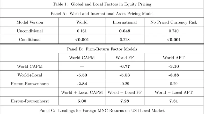
Dumas and Solnik (1995) estimated both unconditional and conditional versions of the world CAPM. They found that while the unconditional version of the model was not rejected, the

(8)

conditional version was rejected. Their results are reported in Table 1, Panel A. The unconditional version of the model is not rejected at a p-value of 0.16, but the conditional version is strongly rejected at a p-value less than 0.001. Furthermore, they strongly reject the hypothesis that the price of global and currency risks are constant, suggesting that the unconditional tests lack power. When they consider the same hypotheses for an asset pricing model that allows for exchange rate risk , the "international asset pricing model" (Adler and Dumas (1983), they …nd that the unconditional version is only marginally rejected at 5% while the conditional version is not rejected. Moroever, the hypothesis that exchange rate risk is not priced is strongly rejected. The general conclusions that exchange rate risk is priced and that the price of risk is time-varying appears in a number of papers including De Santis and Gerard (1997) and Vassalou (2000).

2.1.2 Explaining Firm-Level International Equity Returns

Firm-level stock return behavior presents another dimension of international equity pricing. The World CAPM represents a straightforward extension of the domestic CAPM to the international market. However, as has been demonstrated in the domestic empirical literature (e.g., Fama and French (1992), Carhart (1997), this model does not explain the cross-section of returns as well as a model augmented by factors that depend upon size, the value of the …rm, and possibly momentum. The obvious questioned raised by this evidence is: What model best explains …rm-level returns internationally? Since no empirically implementable theoretical model has yet been derived to explain the importance of factors such as size and value, papers that address this question typically rely on a simple factor structure to explain returns.5 _{The e¤ect on expected equity returns from} risk exposure to these factors are measured empirically by the sensitivity or "factor loadings" to factor-mimicking portfolios

Fama and French (1998) studied an international cross-section of …rm equity returns using a global market factor and a factor based upon book value relative to market value. They found that the value premium, characteristic of US …rm returns, is pervasive in the 13 countries studied. Gri¢ n (2002) included the size factor and also considered whether the e¤ects on equity returns di¤er depending on whether the factors are domestic or foreign. He found that country-speci…c versions

5_{On the other hand, Gomes, Kogan, and Zhang (2003) developed a theoretical model that matches the domestic} empirical …ndings.

(9)

of the three-factor model were more useful at explaining portfolio and individual stock returns than a world three-factor model. Hou, Karolyi, and Kho (2011) provide an extensive analysis of 27,000 stocks from 49 countries to investigate the factors that drive …rm-level returns across countries. The model that best explains variation in returns across these stocks is a multifactor model that depends upon the ratio of cash-‡ow to price as well as momentum. Fama and French (2010) examine returns using size, value, and momentum factors for four regions, considering both integrated and local models. They …nd that the local model explains returns best across three regions.

2.1.3 Global versus Local Factors: The Scope for Diversi…cation

Although studies …nd that local factors are important to explain cross-sectional expected returns, the restriction that intercepts equal zero is usually rejected. Therefore, expected foreign equity returns often cannot be measured with much precision. Nevertheless, the importance of local and country risks in international equity returns together with the low correlation across markets suggests that holding foreign equity can help to reduce the risk of the domestic equity portfolio.

Along these lines, Heston and Rouwenhoerst (1994), hereafter HR, asked whether …rm-level returns are driven by country or industry e¤ects. For this purpose, they studied all of the …rms in the Morgan Stanley Capital International (MSCI) indices of 12 European countries. They grouped these …rms into industries and then considered cross-sectional regressions for each …rm’s return,

Rj_t, according to:

Rj_t = t+ it+ kt +e j

t (6)

where t is a time …xed e¤ect and thus a base level of return at time t, and where it and kt are coe¢ cients on dummy variables if the …rm operates in industry i, or comes from country k, respectively, and ej_t is the …rm-speci…c shock. Instead of choosing country and industry returns as benchmark factors for these returns, they constructed an "average …rm" from an equally weighted portfolio. Using these estimates, they found that the country e¤ect explained an average of 24% across industries while the industry e¤ect only explained an average of 5% across countries. They also discovered that 62% of the variance on an average stock can be eliminated by diversifying across industries within a country, while diversifying across countries within an industry eliminates

(10)

80% of this variance. They concluded that country diversi…cation is more important than industry diversi…cation.

Bekaert, Hodrick, and Zhang (2009) considered various factor models to ask which one best explains the variation in international equity returns for all of the …rms in the MSCI world index. Since …rst moments of equity returns are imprecisely estimated, they focused upon time-varying second moments. They then ran a horse-race both with and without local factors for four di¤er-ent models: the world CAPM, the model augmented with Fama-French factors, an APT model estimated by principal components, and the HR model.

Table 1 B provides some summary information about these tests. The table reports t-statistics for the di¤erence in Mean-Squared-Errors (MSE)6 of the model in the row minus the MSE of the model in the column. Thus, the …rst line shows that the MSE of the World CAPM is signi…cantly higher than both the MSE of the World Fama French (-6.77) and the World APT (-3.10) models. Clearly, the World CAPM is dominated by these other models. However, the second line shows that all of these models are improved by adding local factors. As such, all the versions of models with local factors signi…cantly dominate world-only factor models. Since the HR model inherently imposes the restriction that the factor loadings are e¤ectively one, it does not explain returns as well as any of the other models except the World CAPM.

A number of papers have suggested that industry e¤ects are becoming more important than country e¤ects. These papers include Cavaglia, Brightman, and Aked (2000), Ferreira and Gama (2005), Carrieri, Errunza, and Hogan (2007) and Carrieri, Errunza, and Sarkissian (2008). Bekaert, Hodrick and Zhang (2009) reconciled their results with this literature by testing for di¤erences in trend correlations over time. Using more recent data, they found that country e¤ects are still signi…cantly important in explaining international equity returns even after controlling for industry e¤ects

Another feature of global and local factors is the relatively high comovement between company returns and local factors, as demonstrated by the coe¢ cients on the World plus Local CAPM model. This factor sensitivity a¤ects the ability to diversify internationally. Although Bekaert, Hodrick and Zhang (2009) showed that other models explain returns better, this simple two factor model continues to be a benchmark for many studies that consider international events such as

6

(11)

cross-listings. To illustrate this relationships, Panel C1 reports the cross-sectional mean of a set of time series regressions for all foreign multinational companies that have listed on a US equity exchange since 1975 through 2010, approximately 1100 total. These companies are important because they are the most likely to be globally priced. Nevertheless, a simple mean of coe¢ cients from return regressions of these foreign companies on the US market suggest they would be an excellent hedge since the beta is essentially zero while the coe¢ cient on the local market is about 0.8.

This simple statistic ignores the correlation across US and foreign returns as well as the increase in that correlation over time, however. Even early studies such as Longin and Solnick (1995) showed that the correlation across major countries increased from 1960 to 1990. The evolution toward more integrated equity return exposures has been substantiated in later studies (e.g., Baele (2005), Eun and Lee (2010), Bekaert, Harvey, Lundblad, and Siegel (2007)). This relationship is likely to hold true in …rm returns as well. Indeed, as Panel C shows under section 2, the relationship between the …rm returns and the market returns changes signi…cantly after cross-listing. The table reports results from Chua, Lai, and Lewis (2010) for a market-weighted set of …rms that are listed on US exchanges in 2004. Using a test that endogenously chooses break dates, they found that the foreign …rm betas on the US market increased over time after cross-listing. These results corroborate evidence from a number of authors that condition on cross-listing dates, beginning with Foerster and Karolyi (1999,2000). Section 3 of Panel C restates some of their estimates showing that the average global beta increased after cross-listing while the local beta even declined.7 Thus, while foreign …rms tend to have low betas against the US and other world markets, these betas appear to be increasing over time.

2.2 Local Market Risks and International Equity Pricing Models

Overall, the evidence on international equity returns shows that the standard world CAPM and the associated single factor model of returns is rejected by the data. Empirical international equity pricing studies show that returns depend upon more than a single factor and that at least some of these additional factors depend upon local sources of risk. Developing models to explain both global and local sources of risk is challenging since the two are typically associated with di¤erent

(12)

views of market integration. In the simple framework above, equity prices are either priced in completely segmented markets as in equation (1) so that all factors are local or else they are priced in fully integrated markets as in equation (2) so that all factors are global. The evidence, therefore, poses a challenge to develop models that allow for investors to have access to international markets yet retain exposure to local shocks that cannot be diversi…ed away.

2.2.1 Purchasing power parity deviations and exchange rate risk

Purchasing power parity deviations generate one potential answer to this challenge. In a seminal paper, Adler and Dumas (1983) showed how purchasing power parity deviations a¤ect equity re-turns. Even though investors may trade in fully open capital markets, purchasing power parity deviations imply that the real return to investors vary across countries. As a result, investors view the expected return and risk from investing in securities di¤erently depending upon their country of residence. The pricing of international securities therefore depends upon the covariance of the security returns with the home investor’s in‡ation, a "local" risk factor, and also the covariance of this security’s returns with all the rest of the world’s purchasing power parity deviations, a set of "global" risk factors.

A necessary condition for this model to hold in the data is that exchange rate risk be priced, a condition established in the literature I described above. However, since individual equity returns also depend upon other local factors, currency appears to be only part of the explanation for international equity returns.

2.2.2 Emerging markets and capital market liberalizations

Some governments restrict access to their countries’ capital markets. Since these restrictions segment global capital markets, they provide another reason for local factors to a¤ect equity returns. This explanation was described in theoretical papers as early as Black (1974) and Stulz (1981a). These papers considered the impact on equity returns if the domestic investor must pay extra costs on the foreign relative to domestic investments. Errunza and Losq (1985,1989) developed a framework to consider more direct capital market restrictions among countries. While these papers did not relate the equity returns directly to a world and local factor model, they generally found that the capital market equilibrium returns di¤er across countries and, as emphasized by

(13)

Stulz (1981a), need not correspond to a completely segmented or integrated model.

Bekaert and Harvey (1995) examined this relationship in equity returns of emerging markets. They considered an empirical model that switched between two regimes. In the …rst, markets are completely integrated as in equation (2). Rewriting the stochastic discount factor into components of the world price of risk, the Euler equation (3) under integration implies that the market returns for countryj depend upon the covariance with the world according to:8

Etrtj+1 = tCovt(rjt+1; rWt+1) (7)

where r_tW₊₁ is the return on the world market and t is the time t expected world price of risk. Alternatively, for an emerging market with closed capital markets, the returns within a country are determined solely by their covariance with the domestic market as in equation (1). In this case, the stock market return for countryj is given by:

Etrj_t₊₁ = jtV art(rj_t₊₁) (8)

where j_t is the corresponding price of country j risk. They pointed out that an econometrician analyzing emerging market returns would observe data over both regimes. Thus, the returns would be explained by both the integrated world factor in equation (7) and the segmented local market factor in equation (8) according to:

Etrtj+1= j t tCovt(rjt+1; rtW+1) + (1 j t) j tV art(rjt+1) (9)

where j_tis the probability of countryjbeing in an integrated regime based upon timetinformation. They estimated this model and found that indeed there is time-varying integration generated by the probability of being in the two regimes.

The potential for time-varying integration poses issues for valuing assets in emerging markets. Bekaert and Harvey (1997) considered the implications for measuring volatility and pricing behav-ior. Henry (2000) and Chari and Henry (2008) looked at the impact on aggregate and individual stock returns when markets announce a liberalization. Bekaert and Harvey (2000) consider a

8

(14)

present value model based upon dividend yields to measure the e¤ects on cost of capital from lib-eralization. Bekaert, Harvey, and Lumsdaine (2002) used data on stock market returns together with macroeconomic variables to estimate the date of the liberalization across a number of episodes. They found that the dates estimated with returns align well with the announcements. Surveys of the implications of liberalization on equity pricing and on capital markets perspective are given in Bekaert and Harvey (2003) and in Henry (2007), respectively.

Overall, the empirical equity pricing literature on emerging markets and liberalizations provides one explanation for the presence of global and local factors in returns. These two sets of factors co-exist in returns as countries transition to more open markets. However, transition to openness seems less likely to explain the importance of local and global factors in equity returns of developed countries.

2.2.3 Information Di¤erences across Markets

Equity returns depend upon both global and local sources of risk. These sources of risk can result from di¤ering real returns as with purchasing power parity deviations or explicit restrictions to capital movements as with emerging markets. However, these sources of risk can also arise from more subtle impediments such as informational di¤erences across international markets.

Several papers developed asymmetric information models to consider international investment ‡ows. The basic model in Brennan and Cao (1997) has become a benchmark for this literature. In this model, domestic and foreign investors receive public and private signals about payo¤s on investments in the home and foreign market. The precision of the signals to investors is higher in their own market, capturing the idea that these investors have more information about home securities. A random supply of exogenous "liquidity traders" arrive every period, purchase the assets, and help determine the price. Thus, the equilibrium price depends upon the signals of the two sets of investors. While the models in this literature are developed to explain investment ‡ows rather than returns per se, the stock price solutions illustrate the intuition that asymmetric information will generate both local and foreign risk factors in returns.

Dumas, Lewis and Osambela (2010) considered whether di¤erences in the ability to assess information across countries can generate an asset pricing model with local and global risk factors, among other empirical regularities. In their model, domestic and foreign investors observe signals

(15)

about the expected growth of dividends. In contrast to the asymmetric information literature, all signals are public but domestic investors understand better how to use that information to forecast future dividends. Since investors react to the same information di¤erently, this behavior induces an additional source of risk. The model implies that returns have a two-factor structure that depends upon both home consumption and foreign consumption. Moreover, the equilibrium equity returns depend upon all of the state variables in their model, including up to seven factors, consistent with the number of factors found in Bekaert, Hodrick, and Zhang (2009).

2.2.4 International Equity Pricing Overview

No single asset pricing model appears to …t the empirical result that returns are simultaneously priced with local and global factors across a wide range of countries and …rms. Nevertheless, there is some support for each explanation. Equity returns appear to include the pricing of foreign exchange, consistent with the importance of in‡ation di¤erences. Equity returns from emerging markets depend upon a combination of segmented and integrated market risks and the shifts in these patterns correspond to liberalization dates. Finally, di¤erences in information across markets generate sources of domestic and foreign risks that should theoretically be priced in equilibrium, though these risks are di¢ cult to measure.

2.3 Other Implications of Equity Pricing Models

So far, I have described research related to international equity pricing relationships. But many of the models used to describe these relationships have other capital market implications as well. I next highlight three of these: home equity preference by investors; the relationship between international capital ‡ows and returns; and equity responses to international cross-listing.

2.3.1 Home Equity Preference

Domestic investors hold a disproportionate share of their equity portfolio in domestic …rms. This observation was noted in the US at least as early as Grubel (1968) and Levy and Sarnat (1970) and was shown in a data set across several developed countries by French and Poterba (1991). Moreover, Ahearne, Griever, and Warnock (2004) have shown that the proportion of foreign equity

(16)

holdings in the US portfolio is only about 12%, while the foreign portfolio share in world markets is about 50%. Thus, the so-called "home bias" phenomenon appears to persist.

Whether this phenomenon is puzzling clearly depends upon how well the domestically-biased portfolios achieve the objectives of home investors. If international equity returns are determined by a single factor model such as the World CAPM, then domestic investment in foreign equities indeed fall short of the optimal holdings implied by a market-weighted share of foreign equities in the world portfolio. However, as described above, the literature on international equity pricing demonstrates that this simple version of the model is rejected by the data. Thus, whether home equity preference is surprising must be put into the context of other asset pricing models that can potentially …t the data better. Toward this purpose, I now reconsider home equity preference in the context of the asset pricing models described above.9

One reason why investors may hold di¤erent portfolio allocations than the world market portfolio is that returns di¤er according to the country of residence. In their seminal paper, Adler and Dumas (1983) derived the equilibrium portfolio holdings for investors facing purchasing power parity deviations and, hence, real exchange rate risk. The desired portfolio for an investor in a given country depends upon two components: a common portfolio across investor that maximizes the log of mean gross returns and a country-speci…c portfolio that hedges the real exchange rate risk. Cooper and Kaplanis (1994) combined moments of equity returns and portfolio holdings to ask whether currency risk can explain home bias. They found that it cannot. They then used their estimates to back out the size of implicit transactions costs required to prevent investors from holding these positions. These estimates appear unrealistically high.

While country-speci…c risk in the form of real exchange rate variation may not be su¢ cient to explain home bias, investors may consider other idiosyncratic risks that may be diversi…ed with foreign assets. These country-speci…c risks may include shocks to non-tradeable goods (Baxter, Jermann, and King (1998)) and human capital (Baxter and Jermann (1997), Jermann (2002)).

Whether these argument help or hurt the home equity bias explanation depends upon how well foreign assets hedge these country-speci…c risks relative to domestic assets. If domestically traded assets can provide diversi…cation opportunities without the need to directly invest in foreign assets,

9

A full survey of home equity preference is beyond the scope of this paper. For a longer but dated survey, see Lewis (1999). Coeurdacier and Rey (2010) give an excellent recent survey of home bias in macroeconomic models.

(17)

even small transactions costs and informational asymmetries may induce investors to overweight domestic equities. To investigate this possibility, Errunza, Hogan, and Hung (1999) constructed optimally weighted portfolios of US-traded securities that are likely to have foreign risk components, securities such as US multinationals, foreign stocks listed on US exchanges (ADRs), and country funds. They then tested whether these US-traded portfolios span the risk in foreign market indices. Interestingly, they could not reject this hypothesis except for some of the emerging markets. Their results call into question the bene…ts of holding foreign equities directly on foreign stock exchanges since this diversi…cation can be duplicated on the domestic exchange with lower transactions costs. Stocks from emerging markets form an exception to this result, but for these stocks capital market restrictions may be more signi…cant.

Another potential problem with the standard home equity preference argument involves the time-varying variances of international equity returns. A number of papers such as King, Sentana, and Wadhwani (1994), and Longin and Solnik (1995, 2001) showed that the correlation between in-ternational equity returns are higher when the market declines than when it increases. If so,argued Ang and Bekaert (2002), the diversi…cation potential of foreign equity may be diminished since cor-relations are high when hedging motives are most needed. Nevertheless, these authors showed that the bene…ts of international diversi…cation remained during bear markets as well as bull markets. On the other hand, Chua, Lai, and Lewis (2010) showed that foreign equities traded in the US would not have provided diversi…cation bene…ts during the recent …nancial crisis.

Finally, asymmetric information between domestic and foreign investors may generate a ten-dency to hold domestic assets. Gehrig (1993) showed that if domestic investors have more precise information about home equity compared to foreign investors, they will choose to hold relatively more domestic equity. Intuitively, foreign stocks will seem riskier because domestic investors are less informed about them. In this framework, home bias stems from the assumption that domestic investors are more informed about domestic securities, leading one to ask why foreign investors do not become more informed about the domestic securities.

To address this question, Van Nieuwerburgh and Veldkamp (2009,2010) developed a model in which investors choose how informed they wish to be about a group of assets. In this model, domestic investors have more initial information about the domestic asset so that they have a comparative advantage in local information acquisition. In equilibrium, they endogenously choose

(18)

to remain less informed about the foreign assets in favor of domestic assets.

This line of research would seem to suggest that home bias results simply from an informational disadvantage in foreign assets. However, Dumas, Lewis, and Osambela (2011) showed that this view is too simplistic. In their model, foreign investors have an informational disadvantage in processing domestic signals.10 As such, they overreact to domestic dividend changes. The foreign investor views the domestic equity as being riskier because he does not understand how to interpret all the publically available information. The presence of confused foreign investors creates sentiment risk in domestic equity returns, thereby reducing desired domestic equity holdings by domestic investors. Dumas, Lewis, and Osambela (2011) found that the informational advantage e¤ect dominates the foreign sentiment risk e¤ect on average, but that these two e¤ects generate time-varying home bias.

2.3.2 Foreign capital in‡ows and equity returns

The relationship between capital ‡ows and equity returns is another relationship that depends upon global asset pricing. Bohn and Tesar (1996) found that monthly US portfolio ‡ows are positively related to contemporaneous ‡ows in most large equity markets. The standard asset pricing model with complete information and markets provides little guidance about capital ‡ows since prices can equilibrate without any associated capital ‡ows. By contrast, asset pricing models based upon asymmetric information generate capital ‡ow predictions as investors attempt to trade on their private information.

Brennan and Cao (1997) developed these implications by assuming that investors in the home country have access to more precise private signals about domestic dividend pay-outs. As a result, foreign investors over-react to common public signals, thereby creating a positive correlation between domestic returns and foreign capital in‡ows. They empirically studied this relationship for both developed and emerging markets. Similar to Bohn and Tesar(1996), they found that the purchases of US equities by foreign developed countries and US purchases of equities in these same countries were generally positively related to returns, though the results were more mixed for emerging markets. Using a model with international di¤erences in opinion described above, Dumas, Lewis, and Osambela (2011) also generate covariation between domestic returns and foreign

1 0_{This informational assumption builds on the frameworks in Dumas, Kurshev, and Uppal (2009) and Scheinkman} and Xiong (2003).

(19)

capital in‡ows.

While the Brennan and Cao (1997) model implies a contemporaneous movement between returns and capital ‡ows, in practice empirical studies relate lagged capital ‡ows to contemporaneous returns in order to adjust for information lags. As such, the relationship is typically associated with "trend-following" behavior by foreigners, as found in several papers.11 Brennan, Cao, Strong, and Xu (2005) argued that di¤erences in lags of portfolio ‡ows make the trend-following evidence di¢ cult to interpret. Instead, they used surveys of institutional investors to study how market returns across countries a¤ect the "bullishness" of these investors. Consistent with their model, they found that the fraction of foreign institutional investors that are bullish about a given market increases with the return on that market. However, Curcuru, Thomas, Warnock, and Wongswan (2011) examined newly available data on country allocations and showed that U.S. investor trades are consistent with portfolio rebalancing, not with an informational advantage.

Baker, Wurgler and Yuan (2010) examined more directly the empirical implications of poten-tial di¤erences of opinion on international returns. Following the approach taken by Baker and Wurgler (2006) for US alone, they constructed a "Sentiment Index" for six developed countries using principal components of several data variables related to bullishness of the market. They then used the common component across these markets to characterize a global sentiment index. They found that the global sentiment index rather than the local sentiment index was important for explaining the cross-section of returns. As they argued, capital ‡ows are one mechanism for this sentiment to spread across countries.

2.3.3 International equity cross-listing

The stock price response of …rms that cross-list in other markets is often cited as evidence of market segmentation. For example, Table 1 Panel C3 reports the abnormal returns from Foerster and Karolyi (1999) for the window of one year prior to the cross-listing event at about 15 basis points weekly or about 7% annually. The listing week displays another 12 basis point increase (not shown), and then the returns decline by about 14 basis point, though not signi…cantly. As

1 1_{See for example, Froot, O’Connell, and Seasholes (2001), Choe, Kho, and Stulz (1999, 2005), Grinblatt and} Keloharju (2000), Gri¤en, Nardari, and Stulz (2004), Edison and Warnock (2008), and Dahlquist and Robertsson (2004). However, Grinblatt and Keloharju (2000) …nd that foreign institutional investors make more pro…ts on their investments.

(20)

surveyed in Karolyi (2006), this pattern is robust. Across a variety of studies, returns on stocks tend to be abnormally high around their cross-listing event with estimates ranging from 1:5%and

7% per annum. Even with an event window as long as ten years, Sarkissian and Schill (2009)

found signi…cant abnormal returns.

The dramatic e¤ect on …rm returns raises obvious questions about the reason. Obvious ex-planations such as risk-sharing are easily ruled out. As described by Karolyi (2006), …rms do not appear to be motivated by lower beta in the US. Indeed, most of the cross-listed …rms come from countries such as Canada that already comove strongly with the US. However, the biggest price e¤ects are documented for …rms from countries with more lax disclosure requirements than the US. Co¤ee (2002) argued that these e¤ects are generated by a "bonding" e¤ect. Foreign cross-listed companies bond themselves to a more stringent set of disclosure requirements by committing to abide by US GAAP and regulations from the SEC. As a result, the market views these …rms as less risky and accordingly their stock price rises.

2.4 International Equity Market Summary

Equities comprise an important global asset market. Despite the increase in integration across countries over time, equity returns continue to depend strongly on local factors. Models developed to understand this codependency range from country-speci…c risks, like exchange rates, to capital market restrictions and informational asymmetries. These models also highlight some well-known regularities in these markets such as home bias, the comovement of returns and foreign capital ‡ows, and international equity cross-listing. These models provide a context for considering other global asset markets such as currency and …xed income.

3 Foreign Exchange and International Bond Returns

Currency is an obvious risk characteristic that distinguishes one country’s return from another. Indeed, exchange rate risk appears to be priced in international equity returns, as described above. The price of exchange rate risk can be addressed directly by analyzing the expected return from borrowing in one currency and investing in another currency. Standard foreign exchange risk models treat the borrowing and investing interest rates as short term risk-free rates. However, as

(21)

recent concerns regarding Europe have shown, returns across countries can also embody sovereign default risk as well as potential credit risk di¤erences. In this section, I begin by describing the behavior of foreign exchange returns and its associated literature before turning to the implications for sovereign default risk.

3.1 Foreign Exchange Returns: Structure and Empirical Evidence

Foreign exchange returns are typically characterized by a long-short strategy often used to motivate interest parity. The investor borrows at a domestic currency nominal risk free rate, owing gross return Rerf_t , and then invests the proceeds per unit of domestic currency in a foreign nominal risk-free asset earning gross return Rerf_t in foreign currency units. Thus, the investor engaged in such a strategy will earn St+1Rerft = StRerft in units of domestic currency, where St is the spot domestic currency price of foreign currency. De…ning the nominal home and foreign currency risk-free rates asit and it, respectively the logarithm of this strategy can be written as:

r_tf x st+1 st+ (it it);

where1 +it ln(Retrf),1 +it ln(Re rf

t ), and where lower-case letters refer to the logarithm of the variable. The forward premium equals the di¤erence between the domestic and foreign interest rate by covered interest parity; that is, ft st =it it. Rewriting this strategy in terms of the

forward rate implied by covered interest arbitrage, the excess returns from the strategy becomes:

rf x_t st+1 ft (10)

The foreign exchange return is therefore equivalent to taking a long position in the foreign currency and short position in the domestic currency. If the foreign currency appreciates relative to the forward rate, the future spot price of foreign currency exceeds the forward rate so that the position generates pro…ts.

If the forward rate is an unbiased predictor of the future exchange rate, then interest parity holds and foreign exchange returns earn zero pro…ts on average. Studies …nd that interest parity holds over long horizons, but shorter term deviations can be signi…cant conditional on interest rates.

(22)

To provide a structure to describe this phenomenon, I …rst restate the Euler equation structure in Section 2. I then use this structure to consider the empirical evidence.

3.1.1 Euler Equation Implications

To consider the foreign exchange return using the Euler equation above, I rewrite the stochastic discount factor in nominal terms12. De…ning the price index of the consumption good in the home country as Pt and that of the foreign country as Pt, the nominal stochastic discount factor for domestic and foreign currency can be written as Qt andQt where:

EtQt+1 Et U0₍_C_t₊₁₎_=P_t₊₁ U0₍_C_t₎_=P_t = 1=Re rf t EtQt+1 Et U0(C_t₊₁)=P_t₊₁ U0₍_C t)=Pt = 1=Rerf_t (11)

Thus, Qt+1 is the intertemporal marginal rate of substitution of one unit of domestic currency

between periodt and t+ 1, and similarly forQ_t₊₁. The spot rate is simply the contemporaneous

ratio of nominal rates of substitution in consumption implying:

(St+1=St) = Qt+1=Qt+1 (12)

Using the risk-free rates in equation (11) and the spot rates in equation (12) the foreign exchange risk premium can be rewritten as:13

EtSt+1 Ft St =Et Q_t₊₁ Qt+1 EtQt+1 EtQt+1 (13)

In other words, the risk premium depends upon the di¤erence between the expected ratio of SDFs and the ratio of their expectations. Euler equation-based explanations.must depend upon variation in this relationship.

1 2

See for example Backus, Gregory and Telmer (1993). The approach can also be written in real terms by including two goods that provide a role for real exchange rate variability. For an early example, see Hodrick and Srivastava (1984).

1 3

Taking the expectation of eqn (12) implies that EtSt+1=St =Et(Qt+1=Qt+1). Using the fact thatFt=St =

Rrf_t =Rrf_t by covered interest parity, equation (11) implies that Ft=St = EtQt+1=EtQt+1. Then,

EtSt+1 Ft

St =

(23)

3.1.2 The Fama Result

Early papers on interest parity noted that the forward rate is not an unbiased predictor of the future exchange rate (e.g., Bilson (1981)). Subsequent papers explored the nature of deviations from interest parity. In an in‡uential paper, Fama (1984) used a regression test to demonstrate the signi…cance of these deviations. The test regresses the change in the spot rate on the forward premium, ft st, as given by:

st+1 = 0+ 1(ft st) +ut+1 (14)

where is the lagged di¤erence, _i are regression coe¢ cients and ut+1 is the residual. The

probability limit of the coe¢ cient on the forward premium can be written:

1 =

Cov[Et st+1;(ft st)]

V ar(ft st)

(15)

Fama (1984) showed that if the coe¢ cient is less than a half, then the variance of expected returns exceeds the variance of the expected change in the exchange rate. In other words, if ₁< 1₂, then

V ar Etrtf x > V ar(Et st+1).14

Studies typically …nd that the estimate of ₁ is not only less than(1=2)but negative.15 Negative

1 implies that the exchange rate is predicted to move in the opposite direction of the forward

premium. Panel A of Table 2 illustrates the basic result for monthly returns between Augsut 1978 and October 2010 for the US dollar relative to three representative currencies, the Japanese Yen, the Swiss Franc, and the British Pound.16 The estimate of ₁ is signi…cantly negative for all three currencies. As a result, the hypothesis that ₁ is less than1=2 is rejected at marginal signi…cance

levels less than 1%.

1 4

To see why, note that the predicted return on foreign exchange can be written asEtrtf x+1 Et[ st+1+ (ft st)],

and the variance of the forward premium can be related to the variance of the expected return on the foreign exchange strategy according to: V ar Etrtf x = V ar(Et st+1) 2Cov[Et st+1;(ft st)] +V ar(ft st). Substituting

equation (15) into this expression and rewriting implies: V ar Etrtf x =V ar(Et st+1) + (1 2 1)V ar(ft st).

Then considering 1< 1

2 shows the result.

1 5_{Surveys of this literature can be found in Lewis (1995), and Engel (1996).} _{Bansal and Dahlquist (2000) and} Burnside, Eichenbaum and Rebelo (2007) found that emerging market returns display di¤erent behavior than devel-oped country returns, although deposit rates in these countries may exhibit sovereign risk making the connection to foreign exchange risk alone unclear.

1 6

All spot rate data are from MSCI through Data stream and forward rates are implied through covered interest parity using Datastream Eurocurrency 30 day deposit rates.

(24)

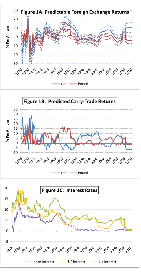
Figure 1A reports the predicted returns for the Yen and Pound against the Dollar based upon this simple regression along with 90% signi…cance bands. The magnitude of the predictable returns is large, sometimes reaching 30% per annum, and changes sign over time.

These two sets of results highlight the challenges for models explaining the foreign-exchange risk premium. First, the model must deliver a negative relationship between the forward premia and future exchange rates, further requiring the variance of the risk premium to exceed the variance of the exchange rate change. In other words, the variance of nominal SDFs in equation (13) must exceed the variance of the ratio of expected nominal SDFs themselves in equation (12). Second, the model must produce the alternating sign pattern of foreign exchange returns found in the data. Therefore, the conditional relationship between SDFs in equation (13) must change signs in a pattern consistent with predictable foreign exchange returns.

For standard consumption-based models to explain the foreign exchange relationship, the con-sumption growth rate must be relatively volatile. However, Panel C of Table 2 shows that the variability of US consumption is only about 1.765% and standard studies …nd this variance is fairly stationary. On the other hand, the variances of foreign exchange returns are typically greater than 20%. The challenge for risk-based models of the foreign exchange risk premium is therefore to generate greater stochastic volatility in the SDFs than readily apparent from casual observation.

3.1.3 The Carry Trade

The negative relationship between the forward premium and the subsequent exchange rate change suggests a simple strategy often called the "carry trade." The forward premium equals the di¤erence between the domestic and foreign interest rate by covered interest parity, i.e,ft st=it it where

it and it are the nominal home and foreign currency risk free rates, respectively.17 Thus, the Fama result says that if the foreign interest rate is higher than the domestic interest rate, the foreign currency is likely to appreciate. The "carry trade" strategy then consists of borrowing in the low-interest rate currencies and investing in the high-interest rate currencies. The carry trade return can therefore be rewritten as: sign(ft st) (st+1 ft).

Table 2 Panel B reports the results from regressing these carry trade returns on the absolute

1 7

These rates are related to the gross returns according to: it it ln(Re rf

t ) ln(Re

rf

(25)

value of the forward premium.18 The coe¢ cients are signi…cant and the mean returns are positive, as reported in the …nal column. Figure 1B illustrates the predicted values of this regression over time for the dollar relative to the Yen and the Pound, while Figure 1C shows the level of interest rates behind this trade. Despite some reversals, the carry trade exhibits prolonged periods of gains. While these …gures report the returns using the dollar interest rate alone, in reality speculators typically use a much wider range of currencies to implement the strategy. Nevertheless, the returns from the strategy are clearly risky.

3.2 Predictable Foreign Exchange Returns Models

Much of the literature has sought to develop models that can generate these relationships between expected returns and interest rate di¤erentials across countries. I begin by describing the mod-els based upon risk-based explanations before considering alternative explanations including rare events, crash risk, and informational asymmetries.

3.2.1 The Foreign Exchange Risk Premium

Any consumption-based model of the foreign exchange risk premium must confront the two chal-lenges I noted above: the higher variance of conditional covariances of SDFs across currencies than the variance of these SDFs themselves; and the changing sign pattern of conditional covariances of SDFs.19 Both of these results require high variability in the marginal utility of consumption. However, early studies beginning with Mark (1985) found that standard consumption volatility is not su¢ cient to generate this foreign exchange risk premium. Backus, Gregory, and Telmer (1993) and Backus, Foresi and Telmer (1993) considered a model with habit persistence that implicitly increased marginal utility variability, but still rejected the model. Bekaert (1996) combined a variety of modi…cations to the standard model including habit persistence and heteroskedasticity, that improved the ability of the model to …t the data. However, the model still could not account for the foreign exchange risk premium. Moreover, as described in Section 2, Euler equation models

1 8_{Similarly, Bansal (1997) found that the coe¢ cient depends on the sign of interest di¤erentials. He also relates} this phenomenon to a term structure model.

1 9

Spot exchange rates provide another problem with these types of models. As a long literature beginning with Meese and Rogo¤ (1983) has shown, exchange rates cannot be explained by standard fundamentals. As labeled by Obstfeld and Rogo¤ (2001), this "exchange rate disconnect problem" continues to plague international macroeconomic models. I do not discuss this literature in the text since exchange rate pricing is inherently a macroeconomic issue and, hence, beyond this review’s scope.

(26)

imply a single latent variable generated by a common SDF, while a large body of research rejects these restrictions.

These early papers focused upon bilateral returns from borrowing in one country and investing in another. However, Lustig and Verdelhan (2007) (LV) formed portfolios of carry trade portfolios according to low relative to high interest rates, rebalanced each year. They found a generally increasing Sharpe ratio in the currencies with higher interest rates. They then used a utility function that nests several di¤erent versions of utility including durables and non-durables and Epstein and Zin (1989) preferences. Based upon this model, they estimated a factor model using US consumption data, …nding that it explains up to 87% of the cross-sectional variation in annual returns on the portfolios. To obtain this result, Lustig, Roussanov, and Verdelhan (2011) showed that the time-varying covariation between the SDF and the global factor is important.

While the LV model focused upon the cross-sectional variation in the predictable excess returns, Lustig, Roussanov, and Verdelhan (2010) examined the time variation in similar portfolios. They found that the predicted foreign currency excess returns are counter-cyclical, using US macro variables. As a result, they demonstrated that the foreign exchange returns portfolios can provide a hedge against cyclical variations so that the predictable returns are, indeed, compensation for risk

Overall, these more recent results suggest that portfolios of foreign exchange returns may have more power to uncover risk-based explanations than the earlier bilateral time series relationships

3.2.2 Rare Events, Crash Premia, and Skewed Returns

Currency markets have a long history of infrequent realignments, as a matter of either explicit or anticipated government reactions. Perhaps not surprisingly, therefore, the impact of rare events on asset prices was …rst noted in foreign exchange markets. According to standard folklore, Milton Friedman coined the term "peso problem" in the early 1970s to describe why Mexican peso interest rates remained substantially higher than the US dollar interest rates even though the exchange rate had been …xed for a decade. The forward rates continued to predict a weaker Mexican peso than was realized until the peso was devalued in the late 1970s.20

2 0_{Empirical analysis of this phenomenon …rst appeared in Rogo¤ (1980) and Krasker (1980).} _{Lizondo (1983)} provided a theoretical model.

(27)

Clearly, the potential for rare devaluations appears most prominent in currencies with …xed exchange rates. However, the term has also been applied when discrete changes are anticipated in asset prices other than currency.21 Moreover, ‡exible exchange rates also appear to experi-ence infrequent shifts. For example, studies such as Engel and Hamilton (1990) and Kaminsky (1993) found that the dollar exchange rate follows persistent regimes of appreciation and deprecia-tion. Therefore, Evans and Lewis (1995) asked whether anticipated discrete shifts in exchange rate regimes could explain the forward discount bias. They found that the anticipated switch from an appreciating to a depreciating regime does, indeed, bias downward the ₁ coe¢ cient in the Fama regression by as much as 1and increases the bias in measured risk premium by3%to20%. Still,

the hypothesis that the true ₁ is equal to1 is strongly rejected.

If investors anticipate an infrequent shift in rates, those with exposure to this event would like to buy insurance against adverse e¤ects on utility. Thus, the price of options against this event would be driven up in equilibrium. This relationship is the insight of Bates (1996a,1996b). He showed that infrequent exchange rate jumps are necessary to explain the higher price of out-of-the money options, the so-called "volatility smile." However, the jumps priced in the options do not appear to predict actual rates, though this …nding may re‡ect the short sample period. A number of studies also found that hedges against jumps appear to be priced in currency and other option prices.22

More recently, Burnside, Eichenbaum, Kleshchelski, and Rebelo (2011) and Jurek (2009) used options data to reexamine the foreign exchange return by combining it with hedged positions. They characterized the position as the combination of a "carry trade", borrowing in the low interest rate and investing in the high interest rate currency, plus an option to hedge against the possible depreciation in the high interest rate currency. Burnside,et al (2011) examined these returns using at-the-money options for a sample ending before the …nancial crisis, …nding signi…cant positive gains. Jurek conducted his analysis over various out-of-the-money strike prices and included a sample extended through the …nancial crisis period of 2008. While the hedged carry trades earned positive Sharpe ratios through 2007, he found that excess returns to crass-neutral carry trades were

2 1

The peso problem has been considered as an explanation of asset pricing behavior ranging from the term premium (Bekaert, Hodrick, and Marshall (2001), Evans and Lewis (1994), to IPO underpricing (Ang, Gu, and Hochberg (2007). For more references see Lewis (2008).

(28)

insigni…cantly di¤erent from zero once the crisis was taken into account. The pattern of positive returns that are eliminated once an infrequent event occurs is consistent with a peso problem explanation.

The original Mexican "peso problem" was envisioned as an e¤ect on the forward premium that would arise even with risk neutral investors. As such, the early literature typically treated the risk premium as an exogenous persistent component to predictable excess returns or as an empirical characterization of the risk-neutral distribution in options. However, risk averse agents would want to hedge against the utility loss from a rare disaster event, thus generating a premium to positions that bear the risk. This observation was made in the context of the equity premium puzzle by Rietz (1988) and more recently restated by Barro (2006). Along these lines, Farhi and Gabaix (2009) proposed a model of a rare global event that a¤ects all countries, but with a di¤ering mean-reverting risk exposure by country.23 They combined these two ingredients to show that those countries more exposed to disaster risk commanded higher risk premia manifested in a depreciated exchange rate and higher interest rate. As the risk premium mean reverts, the exchange rate appreciates so that currencies with higher interest rates appreciate, consistent with the Fama result.

Farhi, Fraiberger, Gabaix, Ranciere and Verdelhan (2009) developed a framework for assessing the importance of disaster risk in currency markets using currency options and foreign exchange returns. They combined both the insights from the cross-sectional behavior of portfolios of carry trades as in Lustig, Roussanov, and Verdelhan (2009) and the disaster risk story in Farhi and Gabaix (2009) to evaluate disaster risk. For this purpose, they used a two country, two period model of disaster risk and considered both hedged and unhedged carry trade returns as in Jurek (2009). They found evidence in favor of the link between exchange rates and asymmetries in the option prices, but more limited evidence of exchange rate predictability, similar to Bates (1996a,b). Brunnermeier, Nagel, and Pedersen (2009) showed that carry trades exhibit negative skewness. That is, most of the time carry trades earn a positive return but infrequently there are large reversals. One interpretation of their results is that carry trade positions are subject to "liquidity spirals" (Brunnermeier and Pedersen (2009)). According to this explanation, speculators invest in these positions because they have positive average return. However, these positions are also

2 3

In the standard model, exchange rates are simply determined by the contemporaneous marginal utility between goods. To generate a forward-looking exchange rate, Farhi and Gabaix (2009) assumed that the exchange rate is a discounted present value of future export productivity.

(29)

subject to "crash risk" captured by negative skewness in these returns. Since these speculators have funding constraints, shocks that lead to losses are ampli…ed as they unwind their positions. The authors indeed found that carry trade positions are positively related with trading volume in futures positions, consistent with their story.

3.2.3 Heterogeneous Investors

The endurance of the forward discount bias and the apparent pro…tability of the carry trade has led some researchers to consider models with heterogeneous investors.

Alvarez, Atkeson, and Kehoe (2008) considered a model that assumes investors di¤er in their …nancial market participation. In their model, households must pay a …xed cost to participate in the …nancial market. Those who pay the cost are active, but the others simply consume current real balances. The model generates a relationship between money growth and the risk premium though it is unclear how much of the forward discount bias can be explained by this relationship.

Osambela (2010) develops a model that allows for domestic and foreign investors to di¤er in their beliefs about the information content of publicly observed signals. He shows that the Fama regression omits one regressor: a heterogeneous beliefs risk premium, which compensates for deviations in beliefs about the expected exchange rate depreciation. He then simulates his model and reruns the Fama regression, …nding that the slope coe¢ cient is biased downward away from one.

3.2.4 Other Low Frequency Movement Explanations

Infrequent crashes in currency markets with or without consumption-based micro-foundations form the basis for the models described above. These stories suggest that a low frequency factor may help explain foreign exchange returns. Similarly, motivations for persistent underlying risk in asset markets have been proposed to help explain well-known domestic market anomalies such as the equity premium puzzle (Mehra and Prescott (1985)) and the risk-free rate puzzle (Weil (1989)). The two main approaches in this line of work are based upon the habit-persistence framework of Campbell and Cochrane (1999) and the long-run risk speci…cation of Bansal and Yaron (2004). While the two approaches di¤er, they both generate low-frequency variability in the stochastic discount factor. Given the importance of low-frequency risk in currency markets, researchers have