Time-Dependent Route Planning
?Daniel Delling and Dorothea Wagner
Universit¨at Karlsruhe (TH), 76128 Karlsruhe, Germany,{delling,wagner}@ira.uka.de
Abstract. In this paper, we present an overview over existing speed-up techniques for time-dependent route planning. Apart from only explaining each technique one by one, we follow a more systematic approach. We identify basic ingredients of these recent techniques and show how they need to be augmented to guarantee correctness in time-dependent networks. With the ingredients adapted, three efficient speed-up techniques can be set up: Core-ALT, SHARC, and Contraction Hierarchies. Experiments on real-world data deriving from road networks and public transportation confirm that these techniques allow the fast computation of time-dependent shortest paths.
1 Introduction
Finding the quickest connection in transportation networks is a problem familiar to anybody who ever travelled. While in former times, route planning was done with maps at the kitchen’s table, nowadays computer based route planning is established: Finding the best train connection is done via the Internet while route planning in road networks is often done using mobile devices. An efficient approach to tackle this problem derives from graph theory. We model the trans-portation network as a graph and apply travel times as a metric on the edges. Computing the shortest path in such a graph then yields the provably quickest route in the corresponding transportation network. In principle, Dijkstra’s classical algorithm [13] can solve this problem. However, for continental-sized transportation networks (consisting of up to 45 million road seg-ments), Dijkstra’s algorithm would take up to 10 seconds for finding a suitable connection, which is way too slow for practical applications. Roughly speaking, Dijkstra computes the distance to all possible locations in the network being closer than the target we are interested in. Clearly, it does not make sense to compute all these distances if we are only interested in the path be-tween two points. Hence, many speed-up techniques have been developed within the last years. Such techniques split the work into two parts. During anoffline phase, called preprocessing, we
compute additional data that accelerates queries during theonline phase. By exploiting several
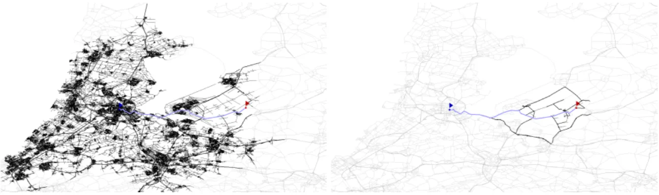
properties of a transportation network, the fastest techniques can obtain the quickest path in road networks within microseconds for the price of few hours of preprocessing. See Fig. 1 for an example of the search space of a speed-up technique compared to Dijkstra’s algorithm.
Up to the year 2008, research on route planning focused either on efficient speed-up tech-niques for time-independent route planning in road networks or on modeling issues (combined
with basic algorithms for determining the best connection) in time-dependent networks deriv-ing from public transportation. For an overview on time-independent route plannderiv-ing, see [10], while [28] presents the work for public transportation. Recently, the focus has shifted to the development of efficient route planning algorithms for time-dependent networks, both road net-works and public transportation. It turned out that switching from a static to a time-dependent scenario is more challenging than one might expect: The input size increases drastically as travel times on time-dependent connections change frequently during the day. Moreover, short-est paths heavily depend on the time of departure, e.g., during rush hours it might pay off to avoid highways. On the technical side, the most efficient time-independent speed-up techniques ?Partially supported by the Future and Emerging Technologies Unit of EC (IST priority – 6th FP), under
Fig. 1.Search space of different algorithms for the same sample query in a road network. The left figure depicts the search space of Dijkstra, the right one for a speed-up technique, i.e., SHARC [2]. Black edges are touched by algorithms, grey ones stay untouched. The shortest path is drawn thicker. We observe that the speed-up technique touches considerably fewer edges than Dijkstra.
rely on bidirectional search, i.e., a second search is started from the target. However, this con-cept is complicated in time-dependent scenarios as the arrival time would have to be known in advance for such a procedure.
Our Contributions. In this work, we recap the recent development on speed-up techniques
for time-dependent route planning covering work from [1, 6–9, 26]. Apart from only explaining the techniques one by one we take a step back and re-analyze them. It turns out that the approach is the same for all time-dependent speed-up techniques: Augment the basic subrou-tines of preprocessing and the query algorithm such that correctness can still be guaranteed in time-dependent networks. Interestingly, all efficient techniques rely on four basic ingredients: Dijkstra’s algorithm [13], landmarks [15, 16], Arc-Flags [21, 22], and contraction [29]. We here explain each ingredient in detail, how they are augmented, and how the recently developed speed-up techniques from combining some of these ingredients are obtained.
Summarizing, in this paper we not only give a survey on time-dependent speed-up techniques but also reinterpret existing results so that the field on the whole becomes clearer to somebody who is new to time-dependent route planning.
Overview. This paper is organized as follows. First, we settle basic definitions in Section 2. In
Section 3, we identify basic concepts for accelerating shortest path queries, show how they can be augmented so that correctness can be guaranteed in time-dependent networks, and analyze their drawbacks. Setting up efficient speed-up techniques from the (augmented) ingredients is done in Section 4. More precisely, we focus on three speed-up techniques: Core-ALT, SHARC, and Contraction Hierarchies. All three approaches are evaluated in Section 5 with real-world transportation networks and Europe. We conclude our work on time-dependent route planning by a summary and a discussion on future work in Section 6.
2 Preliminaries
An (undirected) graphG= (V, E) consists of a finite setV ofnodes and a finite setE of edges.
An edge is an unordered pair {u, v} of nodes u, v ∈ V. If the edges are ordered pairs (u, v), we call the graph directed. In this case, the node u is called the tail of the edge, v the head.
Throughout the whole work we restrict ourselves to directed graphs which are weighted by a length functionlen. The number of nodes|V|is denoted byn, the number of edges|E|bym. We
say a graph issparse ifm∈O(n). Given a set of edgesH,tails(H) /heads(H) denotes the set of all tails / heads inH. With degin(v) / degout(v) we denote the number of edges whose head
/ tail is v. The reverse graph ←G−= (V,←E−) is the graph obtained from G by substituting each (u, v)∈E by (v, u). The 2-core of an undirected graph is the maximal node induced subgraph of minimum node degree 2. The 2-core of a directed graph is the 2-core of the corresponding simple, unweighted, undirected graph. A tree on a graph for which exactly the root lies in the 2-core is called anattached tree. All nodes not being part of the 2-core are called 1-shell nodes. Time-Dependency. We model time-dependency by using functions for specifying edge weights.
Throughout the whole work, we restrict ourselves to a function space F consisting of positive
periodic functionsf :Π →R+, Π = [0, p], p∈Nsuch thatf(0) =f(p) andf(x) +x≤f(y) +y for anyx, y∈Π, x≤y. Note that these functions respect the FIFO property (also called the non-overtaking property) which states that ifAleaves the nodeuof an edge (u, v) beforeB,B cannot
arrive at node v before A. Computation of shortest paths in FIFO networks is polynomially solvable [20]. In non-FIFO networks, complexity depends on the restriction whether waiting at nodes is allowed. If waiting is allowed, the problem stays polynomially solvable; otherwise, the problem is NP-hard [27].
In the following, we call Π theperiod of the input. We restrict ourselves to directed graphs
G= (V, E) with time-dependent length functionslen:E→F. We uselen:E×[0, p]→R+to evaluate an edge for a specific departure time. Note that our networks fullfill the FIFO-property if we interpret the length of an edge as travel times due to our choice of F. The composition of two functions f, g ∈ F is defined by f ⊕g := g◦f. Moreover, we need to merge functions,
which we define by min(f, g) with min(f, g)(x) := min{f(x), g(x)}, x∈Π. The upper bound of f is noted by f = maxx∈Πf(x), the lower by f = minx∈Πf(x). An underapproximation ↓f of
a function f is a function such that ↓f(x) ≤f(x) holds for allx ∈ Π. An overapproximation ↑f is defined analogously. Bounds and approximations of our time-dependent edge functionlen are given by analogous notations. Obviously, one can obtain a time-independent graphG from a time-dependent graph Gby substituting the time-dependent length function by len. We call Gthe lower bound graph ofG.
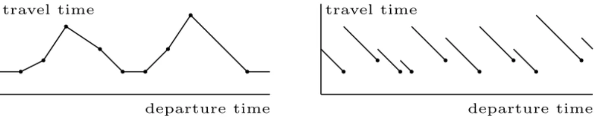
We use piecewise linear functions for modeling time-dependency in transportation networks. Each edge gets a number of interpolation points assigned that depict the travel time on this edge at the specific time. Interestingly, evaluating a function depends on the type of network we use. In road networks, evaluating a function at time τ is done by linear interpolation between the points left and right toτ. In railway networks, we identify the pointpright toτ and return the travel time atp plus the waiting time. Figure 2 gives an example.
Paths. A path P in G is a sequence of nodes (u1, . . . , uk) such that (ui, ui+1) ∈ E for all 1 ≤i < k. In time-independent scenarios, the length of a path is given by Pk−1
i=1 len(ui, ui+1). A path between two nodessandtwith minimum length is called ashortest s–tpath. Byd(s, t)
departure time travel time
departure time travel time
Fig. 2.Examples of piecewise linear travel time functions, the left figure shows a function used for road networks, while the right one is applied to railway networks. Interpolation points are depicted by dots. Note that the evaluation between two points is done in a different manner.
we denote the length of such a path. In time-dependent scenarios, the length γτ(P) of a path
P departing from u1 at timeτ is recursively given by γτ((u1, u2)) =len((u1, u2), τ)
γτ((u1, . . . , uj)) =γτ((u1, . . . , uj−1)) +len
(uj−1, uj), γτ((u1, . . . , uj−1))
In other words, the length of the path depends on the departure time from s. In a time-dependent scenario, we are interested in two types of distances. On the one hand, we want to compute the shortest path between two nodes for a given departure time. On the other hand, we are also interested in retrieving the distance between two nodes for all possible departure
times ∈Π.
By d(s, t, τ) we denote the length of the shortest paths, t∈V if departing from s at time τ. The distance-label, i.e., the distance betweensand tfor all possible departure times∈Π, is given by d∗(s, t). Note that the distance-label is a function ∈F. In this work, we call a query for determining d(s, t, τ) ans-t time-query, while a query for computing d∗(s, t) is denoted by s-tprofile-query.
3 Ingredients and their Augmentation
In this section, we identify basic ingredients all existing high-performance speed-up techniques for time-dependent route planning rely on. These are Dijkstra’s algorithm, landmarks, Arc-Flags, and contraction. In the following, we explain each ingredient separately and show how they are augmented so that correctness can also be guaranteed in time-dependent networks.
3.1 Dijkstra’s Algorithm
The classical algorithm for computing the shortest path from a given source to all other nodes in a directed graph with non-negative edge weights is due to Dijkstra [13]. The algorithm maintains, for each nodeu, a labeldistance[u] with the tentative distance fromstou. A priority queueQ contains all nodes that depict the current search horizon around s. At each step, the algorithm removes (orsettles) the nodeufromQwith minimum distance froms. Then, all outgoing edges
(u, v) ofu are relaxed, i.e., we check whetherd(s, u) +len(u, v)< distance[v] holds. If it holds, a shorter path tovvia uhas been found. Hence,v is either inserted to the priority queue or its priority is decreased.
Augmentation. Computingd(s, t, τ) can be solved by a modified Dijkstra [4]: when relaxing
an edge (u, v) we have to evaluate the weight of it for time τ +d(s, u, τ). In our scenario, the running time for evaluating functions is negligible, hence the additional effort for respecting the departure time is negligible as well.
However, computing d∗(s, t) is more expensive but can be computed by a label-correcting algorithm [5], which can be implemented very similarly to Dijkstra. The source node s is ini-tialized with a constant labeld∗(s, s)≡0, any other nodeuwith a constant label d∗(s, u)≡ ∞. Then, in each iteration step, a node u with minimum d∗(s, u) is removed from the priority queue. Then for all outgoing edges (u, v) a temporary label l(v) = d∗(s, u)⊕len(u, v) is cre-ated. Ifl(v)≥d∗(s, v) doesnot hold,l(v) yields an improvement. Hence,d∗(s, v) is updated to min{l(v), d∗(s, v)}andvis inserted into the queue. We may stop the routine if we remove a node u from the queue with d(s, u) ≥d(s, t). If we want to compute d∗(s, t) for many nodes t∈V, we apply a label-correcting algorithm and stop the routine as soon as our stopping criterion holds for allt. Note that we may reinsert nodes into the queue that have already been removed
by this procedure. Also note that when applied to a graph with constant edge-functions, this algorithm equals a normal Dijkstra. An interesting result from [5] is the fact that the running time of label-correcting algorithms highly depends on the complexity of the edge-functions.
In the following, we construct profile graphs (PG), i.e., compute d∗(s, u) for a given source sand all nodesu∈V, with our label-correcting algorithm. We call an edge (u, v) aPG-edge if
d∗(s, u)⊕len(u, v)> d∗(s, v) doesnot hold. In other words, (u, v) is a PG-edge iff it is part of a shortest path from stov for at least one departure time.
Bidirectional Profile Search. As already mentioned, bidirectional search is prohibited for
time-queries as the arrival time is unknown. However, we can directly apply bidirectional search for profile-queries since we investigate all arrival times. Compared to a time-independent
bidirec-tional Dijkstra, we only need to adjust the stopping criterion. Stop the search if the lower bound of the minimum label in the forward queue added to the lower bound of the minimum label in the backward queue is larger than the upper bound of the tentative distance label.
3.2 A∗ Search Using Landmarks (ALT)
Next, we explain the known technique ofA∗ search [17] in combination with landmarks, called ALT[15, 16]. The search space of Dijkstra’s algorithm can be visualized as a circle around the source. The idea of goal-directed orA∗search is to push the search towards the target. By adding a potential π:V →Rto the priority of each node, the order in which nodes are removed from the priority queue is altered. A ‘good’ potential lowers the priority of nodes that lie on a shortest path to the target. It is easy to see thatA∗is equivalent to Dijkstra’s algorithm on a graph with
reduced costs, formally lenπ(u, v) = len(u, v)−π(u) +π(v). Since Dijkstra’s algorithm works
only on nonnegative edge costs, not all potentials are allowed. We call a potential π feasible
if lenπ(u, v) ≥0 for all (u, v) ∈ E. The distance from each node v of G to the target t is the
distance from v to t in the graph with reduced edge costs minus the potential of t plus the potential of v. So, if the potential π(t) of the target t is zero,π(v) provides alower bound for
the distance from v to the targett.
Preprocessing. There exist several techniques [31, 32] to obtain feasible potentials using the
layout of a graph. TheALTalgorithm however, uses a small number of nodes—so called
land-marks—and the triangle inequality to compute feasible potentials. Given a setL⊆V of land-marks and distancesd(l, v), d(v, l) for all nodesv∈V. For a given landmarkl∈L, the following triangle inequalities hold:
d(l, u) +d(u, v)≥d(l, v) and d(u, v) +d(v, l)≥d(u, l)
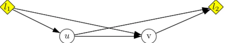
Therefore, d(u, v) := maxl∈Lmax{d(u, l) −d(v, l), d(l, v) −d(l, u)} provides a feasible lower
bound for the distanced(u, v). See Figure 3 for an illustration. The quality of the lower bounds highly depends on the quality of the selected landmarks.
l1 l2
u v
Landmark Selection. A crucial point in the success of a high speed-up when using ALT is the quality of landmarks. Since finding good landmarks is difficult, several heuristics [15, 16] exist. We focus on the best known techniques: avoid andmaxCover.
Avoid [15]. This heuristic tries to identify regions of the graph that are not well covered by the
current landmark setS. Therefore, a shortest-path treeTris grown from a random node r. The weight of each node v is the difference between d(v, r) and the lower bound d(v, r) obtained
by the given landmarks. The size of a node v is defined by the sum of its weight and the size
of its children in Tr. If the subtree of Tr rooted at v contains a landmark, the size of v is set
to zero. Starting from the node with maximum size, Tr is traversed following the child with
highest size. The leaf obtained by this traversal is added toS. In this strategy, the first root is picked uniformly at random. The following roots are picked with a probability proportional to the square of the distance to its nearest landmark.
MaxCover [16]. The main disadvantage of avoid is the starting phase of the heuristic. The first
root is picked at random and the following landmarks are highly dependent on the starting landmark. MaxCover improves on this by first choosing a candidate set of landmarks (using avoid) that is about four times larger than needed. The landmarks actually used are selected from the candidates using several attempts with a local search routine. Each attempt starts with a random initial selection.
Query. The unidirectional ALT-query is a modified Dijkstra operating on the input graph,
the only difference to plain Dijkstra is that the key within the priority queue is not determined only by the distance to sbut also by a lower bound of the distance to the target, given by the landmarks.
It turns out that unidirectional ALT only provides mild speed-ups over Dijkstra’s algo-rithm [11]. The full potential of ALTis unleashed if applied bidirectionally. At a glance, com-bining ALT and bidirectional search seems easy. Simply use a feasible potential πf for the
forward and a feasible potential πb for the backward search. However, such an approach does
not work due to the fact that the searches might work on different reduced costs, so that the shortest path might not have been found when both searches meet. This can only be guaranteed ifπf andπb areconsistent, meaninglenπf(u, v) inGis equal tolenπb(v, u) in the reverse graph. We use the variant of an average potential function [19] defined as pf(v) = (πf(v)−πb(v))/2
for the forward and pb(v) = (πb(v)−πf(v))/2 = −pf(v) for the backward search. By adding
πb(t)/2 to the forward and πf(s)/2 to the backward search,pf and pb provide lower bounds to
the target and source, respectively. Note that these potentials are feasible and consistent but provide worse lower bounds than the original ones.
Augmentation. Based on observation that potentials stay feasible as long as edge weights
only increase and do not drop below their initial values, we can adapt a unidirectional variant of theALTalgorithm to the time-dependent scenario: We perform both landmark selection and distance computation in the lower bound graphG. It is obvious that we obtain a feasible poten-tial. However,ALT implemented as bidirectional search is much faster than the unidirectional variant. As already mentioned, performing a bidirectional search in time-dependent networks is non-trivial. In [26], we showed howbidirectional ALTcan be used in time-dependent networks anyway. The idea is as follows: A backward search is performed inGand is only used to restrict nodes that need to be visited by the forward search.
Bidirectional Query. The query algorithm is based on restricting the scope of a time-dependent
A∗ search from the source using a set of nodes defined by a time-independent A∗ search from the destination, i.e., the backward search is a reverse search in G, which corresponds to the graphGweighted by the lower bounding functionlen. More precisely, it works in three phases: 1. A bidirectional ALTis applied to G, where the forward search is performed on the (time-dependent) graph, and the backward search is run on the lower bound graph G. All nodes settled by the backward search are added to a setM. Phase 1 terminates as soon as the two search scopes meet.
2. Suppose that v ∈ V is a node settled by both searches; then the time dependent cost µ=γτ(pv) of the pathpv going fromstotpassing throughvis an upper bound tod(s, t, τ).
Letβ be the key of the minimum element of the backward search queue; phase 2 terminates as soon asβ > µ. Again, all nodes settled by the backward search are added toM.
3. In the third phase, only the forward search continues, with the additional constraint that only nodes inM can be explored. The forward search terminates whent is settled.
Note that the time-dependent ALT algorithm also works in a dynamic time-dependent scenario: The algorithm still performs accurate queries as long as edge weights do not drop below their lower bound. Moreover, the bidirectional query algorithm can also be used to find a K approximation of the shortest path. Therefore, the second phase is already stopped as soon asβ > Kµ(cf. [26] for details).
3.3 Arc-Flags
The classic Arc-Flag approach, introduced in [21, 22], first computes a partitionC of the graph and then attaches a label to each edge e. A label contains, for each cell C ∈ C, a flag AFC(e)
which is true if a shortest path to at least one node in C starts with e. A modified Dijkstra—
from now on called Arc-Flags Dijkstra—then only considers those edges for which the flag of the target node’s cell is true. The big advantage of this approach is its easy query algorithm.
Furthermore, we observed that for long-range queries in road networks, an Arc-Flags Dijkstra often is optimal in the sense that itonlyvisits those edges that are on the shortest path. However,
preprocessing is very extensive, either regarding preprocessing time or memory consumption.
Preprocessing. Preprocessing of Arc-Flags is divided into two parts. First, the graph is
par-titioned intok cells. The second step then computeskflags for each edge.
Partition. The first approach for obtaining a partition is based on a grid partition [22]. It turns
out that the performance of an Arc-Flags query heavily depends on the partition used. In order to achieve good speed-ups, several requirements have to be fulfilled: cells should be connected, the size of the cells should be balanced, and the number of boundary nodes has to be low. A systematical experimental study of the impact of partitions on Arc-Flags has been published in [25].
Setting Arc-Flags. The second step of preprocessing is the computation of arc-flags. Throughout
the years, several approaches have been introduced (see e.g. [18, 21–24]). We here concentrate on two approaches which turned out to be the most efficient. For both approaches, we have to perform an initialization step, which sets the so-called own-cell flags of all edges not crossing
borders totrue. Note that the own-cell flag of an edge (u, v) in cellC, i.e.,uandvboth are in cell
C, isAFC((u, v)). If uand v are in different cells, no flag is set totrueduring the initialization
Boundary Shortest Path Trees. A true arc-flagAFC(e) denotes whether e has to be
con-sidered for a shortest-path query targeting a node within C. The key observation of this approach is that all shortest paths ending in the cell C must pass any of the boundary nodesBC of cellC. More precisely, a nodeb∈Cis called a boundary node of cellC if there
exists an edge (v, b) ∈ E with node v being part of a cell C0 6=C. With this observation, arc-flags can be computed as follows: Grow a shortest path tree in ←G− from all boundary nodes b∈BC of all cells C. Then set AFC((u, v)) =true if (u, v) is a tree edge for at least
one tree grown from all boundary nodes b∈BC.
Centralized Approach. The drawback of the first approach is that we have to grow |B| shortest path trees yielding long preprocessing times for large transportation networks. [18] introduces a new approach to computing flags. A label-correcting algorithm (also called centralized tree) is performed for each cell C. The algorithm propagates labels of size |BC|
through the network depicting the distances to all boundary nodes of the cell. The algorithm terminates if no label can be improved any more. Then,AFC((u, v)) is set totrueiflen(u, v)+
d(v, b) =d(u, b) holds for at least oneb∈BC.
Query. A unidirectional Arc-Flags query is a modified Dijkstra operating on the input graph.
For anys–tquery, it first determines the target cellT, and then relaxes only those edgesewith
AFT(e) = true. Note that compared to plain Dijkstra, an Arc-Flags query performs only one
additional check.
Note that AFC(e) is true for almost all edges e∈ C due to the own-cell-flag. Due to these
own-cell-flags an Arc-Flags Dijkstra yields no speed-up for queries within the same cell. Even worse, more and more edges become important when approaching the target cell (called the
coning effect) and finally, all edges are considered as soon as the search enters the target cell.
Multi-Level Arc-Flags. While the coning effect can be weakened by a bidirectional approach,
the problem of inner-cell queries persists also for bidirectional search. An approach to remedy this drawback is introduced in [25]: A second layer of arc-flags is computed for each cell. There-fore, each cell is again partitioned into several subcells and arc-flags are computed for each. A multi-level arc-flags query then first uses the flags on the topmost level and as soon as the query enters the target’s cell on the topmost level, the low-level arc-flags are used for pruning.
Preprocessing in a time-independent scenario is done as follows. Arc-flags on the upper level are computed as described above. For the lower flags, grow a shortest path for all boundary nodesbon the lower level. Stop the growth as soon as all nodes in the supercell ofC are settled. Then, we set a low-level arc-flag to true if the edge is a tree edge of at least one shortest path
tree. Note that this approach can be extended to a multi-level approach in a straightforward manner. Also note that multi-level Arc-Flags can be applied bidirectionally as well.
Discusssion. The advantages of Arc-Flags is the easy concept combined with exceptional query
performance: Preprocessing is based on Dijkstra-searches and the query algorithm performs only one additional check (per edge) compared to plain Dijkstra. Stunningly, bidirectional Arc-Flags long-range queries are often optimal—at least in road networks—in that sense thatonly
shortest path edges are relaxed. However, the most crucial drawback of Arc-Flags is its time consuming preprocessing effort. Even the most advanced technique, i.e., the centralized ap-proach, needs more than 17 hours to preprocess a continental-sized road network. Still, due to its superior undirectional query performance, Arc-Flags seemed to be a good starting point for time-dependent shortest path computations.
Augmentation. In time-independent scenarios, a set arc-flag AFC(e) denotes whether ehas
to be considered for a shortest-path query targeting a node within C. In other words, the flag is set ifeis important for (at least one target node) in C. In a time-dependent scenario, we use the following intuition to set arc-flags: an arc-flagAFC(e) is set totrue, if eis important forC
at least once duringΠ. A straightforward adaption of computing arc-flags in a time-dependent graph is to construct a profile graph in←G−for all boundary nodesb∈BC of all cellsC. Then we
setAFC((u, v)) =trueif (u, v) is a PG-edge for at least one PG built from all boundary nodes
b∈BC. In addition, we also set all own-cell flags totrue as well. The time-dependent query is
a normal time-dependent Dijkstra only relaxing edges with set flag for the target’s cell.
Approximation. Computing arc-flags as described above requires to build a complete profile
graph on the backward graph from each boundary node yielding too long preprocessing times for large networks. Recall that the running time of building PGs is dominated by the complexity of the function (cf. Section 3.1). Hence, we may construct two PGs for each boundary node, the first uses↑lenas length functions, the second↓len. Since we use approximations, we may use less interpolations points per label. By this, constructing two such PGs may be faster than building one exact one. We end up in two distance labels per node u, one being an overapproximation, the other being an underapproximation of the correct label. Then, for each (u, v) ∈ E, we set
AFC(u, v) =true iflen(u, v)⊕ ↑d∗(v, bC)>↓d∗(u, bC) does not hold.
If networks get so big that even setting approximate labels is prohibited due to running times, one can even use upper and lower bounds for the labels. This has the advantage that building two shortest-path trees per boundary node is sufficient for setting correct arc-flags. The first uses lenas length function, the other len. Note that by approximating arc-flags (denoted by AF), their quality may decrease but correctness is untouched. Thus, queries remain correct
but may become slower.
Heuristic Arc-Flags. In [8], we proposed a third approach for computing flags. The preprocessing
is as follows: We grow k+ 2 shortest-path trees from each boundary node. The first uses len as metric, the second one len, and the remaining k trees are time-queries in ←G− using a fixed arrival time at the boundary node. We set a flag of an edge for a cellC if the edge is part of at least one shortest path tree grown from the boundary nodes ofC.
Unfortunately, this approach may yield incorrect queries as a shortest path for a specific departure time may have been missed. However, it is obvious that a path is found since at least for one departure time, flags are set totrue for a shortest path to the target’s cell. Experiments
on the eventual error-rate can be found in Section 5.
3.4 Contraction
One reason for the success of hierarchical speed-up techniques is the iterativecontractionof the
input: Unimportant nodes are removed from the graph and additionalshortcuts are inserted to
preserve distances between non-removed nodes.
Node-Reduction. The number of nodes is reduced by iteratively bypassing nodes until no node
is bypassable any more. To bypass a node v we first remove v, its incoming edges I and its
outgoing edges O from the graph. Then, for eachu∈tails(I) and for eachw∈heads(O)\ {u} we introduce a new edge of the lengthlen(u, v)+len(v, w). If there already is an edge connecting u andw in the graph, we only keep the one with smaller length. All nodes not removed by the node-reduction are part of the so calledcore of the input.
1 2 4 3 5 4 2 2 1 4 3 2 2 9 1 4 3 2 2
Fig. 4.Example of contraction. The figure on the left depicts the input, edge labels indicate the weight of the edge. We contract, i.e., remove, node 2 and add an shortcut from node 1 to 4 with weight 9 (middle). However, the shortest path from 1 to 4 is via node 3 with length 4. Hence, we can safely remove the shortcut (1,4) from the core in order to preserve distances between core nodes. The resulting graph is shown on the right.
Edge-Reduction. Note that this node-reduction routine potentially adds shortcuts not needed
for keeping the distances in the core correct. See Figure 4 for an example. Hence, an edge-reduction is performed directly after node-edge-reduction, similar to [30]. We grow a shortest-path tree from each nodeuof the core. We stop the growth as soon as all neighborswofuhave been settled. Then we check for all neighborswwhetheruis the predecessor ofwin the grown partial shortest path tree. Ifu is not the predecessor, we can remove (u, w) from the graph because the shortest path fromutowdoes not include (u, w). In order to remove as many edges as possible we favor paths with more hops over those with few hops.
Augmentation. Time-dependent contraction is very similar to a time-independent one.
Dur-ing node-reduction, new shortcuts (u, w), depictDur-ing the path from u via v tow, get the func-tion len(u, v)⊕len(v, w) assigned. While this is straightforward in principle, one problem of node-reduction in time-dependent road networks is the following: Let P(f) be the number of interpolation points of the functionf ∈F. Then the composed function oflen(u, v)⊕len(v, w), may have up to P(len(u, v)) +P(len(v, w)) number of interpolation points in the worst case. The main problem is that the interpolation points needed for evaluating len(v, w) may change between two interpolation points oflen(u, v). Figure 5 gives an example, for details we refer the interested reader to [7]. This is one of the main problems when routing in time-dependent graphs: Almost all speed-up techniques developed for static scenarios rely on adding long shortcuts to the graph. While this is cheap for static scenarios, the insertion of time-dependent shortcuts yields a high amount of preprocessed data.
For edge-reduction, we build a PG (instead of a shortest path tree) from each node uof the core. We stop the growth as soon as all neighborsvofuhave their final label assigned. Then we check for all neighbors whetherd∗(u, v)< len(u, v) holds. If it holds, we can remove (u, v) from the graph because for all possible departure times, the path fromutov does not include (u, v).
u
v
w
7:00 - 12 min 8:00 - 16 min . . . 7:00 - 11 min 8:00 - 16 min 8:30 - 16 min . . . 7:00 - 24 min 7:45 - 31 min 8:00 - 32 min . . .u
v
w
7:00 - 12 min 8:00 - 16 min . . . 7:00 - 11 min 8:00 - 16 min 8:30 - 16 min . . . 7:00 - 24 min 7:45 - 31 min 8:00 - 32 min . . .Fig. 5.Time-dependent contraction in road networks. Recall that we interpolatelinearly between interpolation points, i.e., the travel time on edge (u, v) at 7:45 is 15 minutes. It is obvious that we have to add interpolation points at 7:00 and 8:00 to the function assigned to the shortcut (u, w). This would result in a travel time from
uto w of 30 minutes when departing at 7:45. However, we arrive atv at 8:00 when departing fromu at 7:45 and arrive at 8:16 at w. So, the travel time fromu tow is 31 minutes instead of 30. Hence, we need to insert an additional interpolation point at 7:45. The reason for this is that the responsible interpolation points for evaluatinglen(v, w) changes when departing fromuat 7:45.
4 Speed-Up Techniques
In this section, we show how to assemble efficient speed-up techniques from the basic ingredients presented in Section 3. More precisely, we explain Core-ALT, SHARC, and Contraction Hier-archies. Due to their clear foundation on basic ingredients, the augmentation of these speed-up techniques is easier than for other approaches.
4.1 Core-ALT
Core-ALT was introduced in [3] and augmented to the time-dependent scenario in [9]. It is a combination of landmarks, bidirectional search, and contraction. As already discussed in Section 3, pureALTsuffers from two major drawbacks. Space consumption is rather high and— even more important—ALT cannot compete with hierarchical approaches—concerning query performance—in transportation networks. In [3], we showed how to remedy both drawbacks without violating the advantages of pure ALT, i.e., easy adaption to dynamic scenarios and robustness to the input. The key idea is to perform an initial contraction step prior to ALT preprocessing. Landmarks are then chosen from the core and landmark distances are also only stored for core nodes. This yields a 2-phase query. During the first phase, a plain bidirectional Dijkstra is performed until the core is reached. Within the core, bidirectionalALTis applied.
Preprocessing. At first, the input graph G= (V, E) is contracted to a graphGC = (VC, EC),
called the core. Then, we compute landmarks on the core and store the distances to and from
the landmarks for all core nodes. After preprocessing the core, we store the preprocessed data and merge the core and the normal graph to a full graph GF = (V, EF =E∪EC). Moreover,
we mark the core-nodes with a flag.
Query. The s-t query is a modified bidirectional Dijkstra, consisting of two phases, both
performed onGF. During phase 1, we run a bidirectional Dijkstra rooted atsandtnot relaxing
edges belonging to the core. We add each core node, calledentrance point, settled by the forward
search to a setS (T for the backward search). The first phase terminates if one of the following two conditions hold: (1) either both priority queues are empty or (2) the sum of the distances to the closest entry points of sandt is larger than the length of the tentative shortest path. If case (2) holds, the whole query terminates. The second phase is an ALT-query, initialized by refilling the queues with the nodes belonging toS andT.
Augmentation. In [9], we augmented Core-ALT to time-dependent networks. The
prepro-cessing is very similar to the time-independent variant. First, we extract a core GC = (VC, EC)
with a time-dependent contraction routine. Then, we merge the core with the original graph to obtain GF = GC ∪G = (V, E∪EC) since VC ⊂ V. Finally, we select landmarks from GC
and compute landmark distances in GC. The query algorithm again consists of two phases,
performed on GF. Due to the fact that the arrival time is unknown, the query algorithm is
slightly more complicated than in the time-independent case.
1. Initialization phase: start a Dijkstra search from both the source and the destination node on GF, using the time-dependent costs for the forward search and the time-independent
costs lenfor the backward search, pruning the search (i.e., not relaxing outgoing edges) at nodes∈VC. Add each node settled by the forward search to a set S, and each node settled by the backward search to a set T. Iterate between the two searches until: (i) S∩T 6=∅or (ii) the priority queues are empty.
2. Main phase: (i) If S ∩T 6= ∅, then start a unidirectional Dijkstra search from the source on GF until the target is settled. (ii) If the priority queues are empty and we still have
S∩T =∅, then start a bidirectional time-dependent ALT (cf. Section 3) on the graph GC,
initializing the forward search queue with all leaves of S and the backward search queue with all leaves ofT, using the distance labels computed during the initialization phase. The forward search is also allowed to explore any node v ∈ T, throughout the 3 phases of the algorithm. Stop whent is settled by the forward search.
In other words, the forward search “hops on” the core when it reaches a node u ∈S∩VC, and “hops off” at all nodes v ∈T ∩VC. Moreover, we use time-dependent bidirectional ALT in case (ii) during the main phase. With the same arguments from Section 3.2, we can use Core-ALT to compute a K-approximation of the shortest path.
4.2 SHARC
SHARC Routing was introduced in [2] and augmented in [8]. It is based on contraction and Arc-Flags combined with a unidirectional query algorithm.
--0-1111 1111 0010 1111 0010 1 2 3 4 5
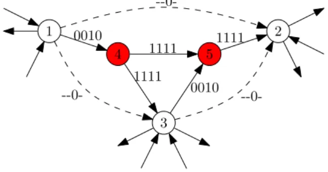
Fig. 6. Example for assigning arc-flags to removed edges during contraction for a partition having four cells. All nodes are in cell 3. The red nodes (4 and 5) are removed, the dashed shortcuts are added by the contraction. Arc-flags (edge labels) are indicated by a 1 for true and 0 for false. The edges heading a node removed by the contraction routine get only their own-cell flag set true. Any other removed edge gets all flags set totrue. The added shortcuts get their own-cell flags fixed tofalse.
Preprocessing of static SHARC is divided into three sections. During the initialization
phase, we extract the 2-core of the graph and perform amulti-levelpartition ofG. Then, an it-erativeprocess starts. At each stepiwe first con-tract the graph bybypassing unimportant nodes
and set the arc-flags automatically for each
re-moved edge, depending on the tail u of the re-moved edge. Ifu is a core node, we only set the own-cell flag totrue(and others tofalse) because
this edge can only be relevant for a query tar-geting a node in this cell. Otherwise, all arc-flags are set totrueas a query has to enter the core in
order to reach a node outside this cell. See Fig. 6 for an example. For the remaining edges of the contracted graph we compute the arc-flags ac-cording to Section 3. In the finalization phase,
we assemble the output-graph, refine arc-flags of
edges removed during contraction, and finally reattach the 1-shell nodes removed at the begin-ning.
Basically, the SHARC query is a modified Dijkstra that operates on the output graph. The modifications are the same as for a multi-level Arc-Flags query (cf. Section 3): When settling a nodeu, we compute the lowest levelion whichuand the target nodetare in the same supercell. When relaxing the edges outgoing fromu, we consider only those edges having a set arc-flag on levelifor the corresponding cell oft. Note that the SHARC query, compared to plain Dijkstra, only needs to perform two additional operations: computing the common level of the current node and the target and the arc-flags evaluation.
Augmentation. The adaption of SHARC [8] is done in a straightforward fashion. We use
time-dependent contraction and time-time-dependent arc-flags computation during preprocessing instead of their time-independent counterparts.
Variants. In Section 3.3, we presented several ways of computing time-dependent arc-flags.
The aggressive variant of SHARC uses exact flags during preprocessing, the economical version uses approximate flags, while heuristic SHARC uses heuristic flags. Hence, aggressive SHARC tends to have long preprocessing times combined with a better quality of flags, while economical SHARC has shorter preprocessing times for the price of worse flags. Heuristic SHARC however cannot guarantee correctness of the queries.
Landmarks. Approximate arc-flags yield worse results than exact ones. In order to partly remedy
this loss in performance, we can add landmarks to SHARC. We can combineALTwith SHARC easily. We run a time-dependent ALT preprocessing consisting of selecting landmarks L ⊆ V and computing d(l, v), d(v, l) for all v ∈V, l∈ L. Then, we apply a normal SHARC-query but used(s, u, τ) +π(u) (cf. Section 3) instead ofd(s, u, τ) as priority key. We call this combination L-SHARC (Landmarks and SHARC).
4.3 Contraction Hierarchies
Contraction Hierarchies (abbreviated by CH) were introduced in [14] and augmented to the time-dependent scenario in [1]. This approach is solely based on contraction combined with a bidirectional query algorithm. Preprocessing is divided into two parts: node-ordering and contraction. Node-ordering assigns a priority to each node depicting its importance in an n-level hierarchy. Then, during contraction, the input graphGis transferred to two search graphs G↑ and G↓, which are called upward and downward graph, respectively. G↑ only stores edges directing from unimportant to important nodes, while G↓ contains only edges directing from important to unimportant nodes. These graphs can be constructed by running n node- and edge-reduction steps similarly to how it is explained in Section 3. However, each node-reduction step contracts exactly one nodeu, resulting in a very limited edge-reduction routine as unneeded shortcuts may only be added between neighbors of u. The query algorithm is conducted of two Dijkstra searches, a forward search (from s) operating on G↑ and a backward search (from t) on G↓.
Augmentation. Contraction Hierarchies is adapted by augmenting the contraction process
with the process of node-ordering untouched. So, time-dependent preprocessing is straightfor-ward; the main challenge is the adaption of the query algorithm.
The basic static query algorithm for CHs consists of a forward search in an upward graph G↑ = (V, E↑) and a backward search in a downward graph G↓. Wherever these searches meet, we have a candidate for a shortest path. The shortest such candidate is a shortest path. Since the departure time is known, the forward search is easy to generalize. The easiest way to adapt the backward search is to explore all nodes that can reach t in G↓. During this exploration all edges connecting nodes that can reach tare marked. Let Emarked denote the set of marked edges. Then, ans–t-query can be performed by a forward search fromsin (V, E↑∪Emarked).
5 Experiments
In this section, we recap experimental results on the performance of time-dependentALT, Core-ALT, SHARC, and Contraction Hierarchies for road and railway networks. The experimental results are taken from [1, 7].
All tests were executed on one core of two similar (with respect to performance) machines, both running SUSE Linux 10.3. The first machine is an AMD Opteron 2218 clocked at 2.6 GHz, has 16 GB of RAM and 2 x 1 MB of L2 cache. The second machine has a Xeon 5345 processors
clocked at 2.33 GHz with 16 GByte of RAM and 2 x 4 MB of L2 cache. All programs were compiled with GCC 4.2.1 or 4.3.2, using optimization level 3.
Inputs. Two types of inputs are applied: Road and railway networks. For the former, we have
ac-cess to a real-world time-dependent road network of Germany. It has approximately 4.7 million nodes and 10.8 million edges. In order to analyze the scalability of our approaches, we addition-ally use the available real-worldtime-independent network of Western Europe (18 million nodes
and 42.6 million edges) and generate synthetic rush hours. All data has been provided by PTV
AG for scientific use. The German data contains five different traffic scenarios, collected from historical data: Monday, midweek (Tuesday till Thursday), Friday, Saturday, and Sunday. As expected, congestion of roads is higher during the week than on the weekend:≈8% of edges are time-dependent for Monday, midweek, and Friday. The corresponding figures for Saturday and Sunday are ≈ 5% and ≈ 3%, respectively. Our railways timetable data—provided by HaCon for scientific use—of Europe consists of 30 516 stations and 179 985 trains. The period is 24 hours. The resulting realistic, i.e., including transfer times, time-dependent network has about 0.5 million nodes and 1.4 million edges, and is fulfilling the FIFO-property.
Setup. In the following, we report preprocessing times and the overhead of the preprocessed
data in terms of additional bytes per node. Moreover, we report two types of queries: time-queries, i.e., queries for a specific departure time, andprofile-queries, i.e., queries for computing
d∗(s, t). For each type we provide the average number of settled nodes, i.e., the number of nodes taken from the priority queue, and the average query time. For s-t profile-queries, the nodes s and t are picked uniformly at random. Time-queries additionally need a departure time τ as well, which we pick uniformly at random as well. As all methods introduced in this chapter have approximate variants, we record four different statistics to characterize the solution quality: error rate, average relative error, maximum relative error, maximum absolute error. By
error rate we denote the percentage of computed suboptimal paths over the total number of
queries. By relative error on a particular query we denote the relative percentage increase of
the approximated solution over the optimum, computed asω/ω∗−1, whereω is the cost of the approximated solution andω∗ is the cost of the optimum computed by Dijkstra’s algorithm. We report average and maximum values of this quantity over the set of all queries. The maximum
absolute error is given by ω−ω∗. All figures in this chapter are based on 100 000 random s-t queries and refer to the scenario that only the lengths of the shortest paths have to be determined, without outputting a complete description of the paths.
5.1 Road Networks
First, we compare all time-dependent algorithms discussed in this paper among each other. We hereby split our comparison in two parts. Exact queries and approximation. Table 1 reports query performance of time-dependent Dijkstra, uni-directionalALT, bidirectional ALT, Core-ALT (CALT), SHARC, and Contraction Hierarchies (CH) for our exact setup, while Tab. 2 depicts performance if suboptimal paths are allowed. As input we use our time-dependent road networks of Europe (high traffic) and Germany (midweek and Sunday). Note that no approximate variant of Contraction Hierarchies exists yet and that no results for Europe (high traffic) have been published. The reason for the latter is the high memory consumption making Contraction Hierarchies impractical for this input.
Exact Setup. Depending on the scenario, different algorithms perform best. While CALT
Table 1.Performance of Dijkstra, uni- and bidirectionalALT, Core-ALT, SHARC, and Contraction Hierarchies (CH) in an exact setup. Note that no figures on the number of relaxed edges are given in [1].
Prepro Queries
time space #delete speed #relaxed speed time speed input algorithm [h:m] [B/n] mins up edges up [ms] up Dijkstra 0:00 0 2 305 440 1 5 311 600 1 1 502.88 1 uni-ALT 0:23 128 200 236 12 239 112 22 148.36 10 ALT 0:23 128 110 134 21 131 090 41 94.26 16 Ger midweek CALT 0:09 50 3 190 723 12 255 433 5.36 280 eco SHARC 1:16 155 19 425 119 104 947 51 25.06 60 eco L-SHARC 1:18 219 2 776 831 19 005 279 6.31 238 CH 0:25 1 019 528 4 366 – – 1.22 1231 Dijkstra 0:00 0 2 348 470 1 5 410 600 1 1 464.41 1 uni-ALT 0:23 128 142 631 16 170 670 32 92.79 16 ALT 0:23 128 58 956 40 70 333 77 42.96 34 CALT 0:05 19 1 773 1 325 6 712 806 2.13 688 Ger Sunday eco SHARC 0:30 65 2 142 1 097 6 549 826 1.86 787 eco L-SHARC 0:32 129 576 4 076 2 460 2 200 0.73 2 011 agg SHARC 27:20 61 670 3 504 1 439 3 759 0.50 2 904 agg L-SHARC 27:22 125 283 8 300 978 5 535 0.29 5 045 CH 0:11 248 407 5 770 – – 0.71 2 061 Dijkstra 0:00 0 8 877 158 1 21 006 800 1 5 757.45 1 uni-ALT 1:15 128 2 143 160 4 2 613 994 8 1 520.83 4 Europe ALT 1:15 128 3 009 320 3 3 799 112 6 1 379.21 4 high traffic CALT 1:00 61 60 961 146 356 527 59 121.47 47 eco SHARC 6:44 134 66 908 133 480 768 44 82.12 70 eco L-SHARC 6:49 198 18 289 485 165 382 127 38.29 150
win with respect to query performance. While CH tend to have fast query times, the space consumption is up to 1 000 bytes per node. For this reason, CH cannot be used for Europe (high traffic). Aggressive SHARC however, has the lowest query times but for the price of high preprocessing times. In fact, preprocessing times for aggressive SHARC are only practical for Germany on Sunday. As soon as the graph gets bigger or more edges are time-dependent, preprocessing takes more than 2 days. So, it seems as if economical L-SHARC and CALT are the techniques most robust to the input. Summarizing, depending on the size of the graph and degree of perturbation, our presented speed-up techniques are 150 to 5 000 times faster than plain Dijkstra. For all evaluated networks, the query performance is sufficient for most real-world environments.
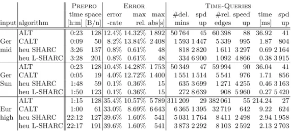
Table 2. Performance of Dijkstra, uni- and bidirectional ALT, Core-ALT, and SHARC in an approximation setup.
Prepro Error Time-Queries
time space error max max #del. spd #rel. speed time spd input algorithm [h:m] [B/n] -rate rel. abs[s] mins up edges up [ms] up ALT 0:23 128 12.4% 14.32% 1 892 50 764 45 60 398 88 36.92 41 Ger CALT 0:09 50 8.2% 13.84% 2 408 1 593 1 447 5 339 995 1.87 804 mid heu SHARC 3:26 137 0.8% 0.61% 48 818 2 820 1 611 3 297 0.69 2 164 heu L-SHARC 3:28 201 0.8% 0.61% 48 334 6 900 1 092 4 866 0.38 3 915 ALT 0:23 128 10.4% 14.28% 1 753 50 349 47 59 994 90 36.04 41 Ger CALT 0:05 19 4.0% 12.72% 1 400 1 551 1 514 5 541 976 1.71 856 Sun heu SHARC 1:48 59 0.1% 0.36% 15 635 3 699 1 271 4 255 0.46 3 163 heu L-SHARC 1:50 123 0.1% 0.36% 15 272 8 639 908 5 960 0.27 5 420 ALT 1:15 128 35.4% 10.57% 5 789 311 209 29 382 061 55 214.24 27 Eur CALT 1:00 61 33.0% 8.69% 6 643 6 365 1 395 32 719 642 9.22 624 high heu SHARC 22:12 127 39.6% 1.60% 541 5 031 1 764 8 411 2 498 2.94 1 958 heu L-SHARC 22:17 191 39.6% 1.60% 541 3 873 2 292 8 103 2 592 2.13 2 703
Approximation. In an approximate scenario, things are clearer. Performance of SHARC is
boosted by more than an order of magnitude if we drop correctness combined with a reasonable preprocessing effort. This very good performance comes together with a very good quality of paths. AlthoughALTand Core-ALTalso gain from allowing suboptimal paths, both query per-formance and quality of paths is (much) worse than for approximate SHARC. We conclude that SHARC is superior if we allow slightly suboptimal paths. Summarizing, approximate SHARC yields speed-ups between 2 700 to 5 420 over Dijkstra’s algorithm combined with very low errors.
5.2 Timetable Information
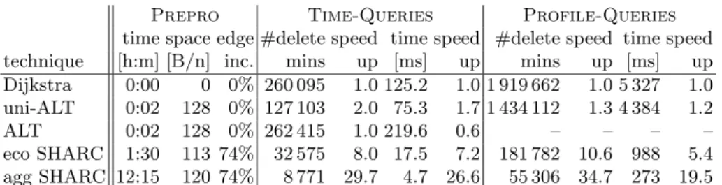
Up to now, Contraction Hierarchies have not been evaluated on graphs deriving from public transportation. Hence, Table 3 shows the results of Dijkstra, uni- and bidirectional ALT, and SHARC for this input.
Table 3.Performance of time-dependent Dijkstra, uni- and bi-directionalALTand SHARC using our timetable data as input. Moreover, we report the increase in edge count over the input.#delete mins denotes the number of nodes removed from the priority queue, querytimes are given in milliseconds.Speed-up reports the speed-up over the corresponding value for plain Dijkstra.
Prepro Time-Queries Profile-Queries time space edge #delete speed time speed #delete speed time speed technique [h:m] [B/n] inc. mins up [ms] up mins up [ms] up Dijkstra 0:00 0 0% 260 095 1.0 125.2 1.0 1 919 662 1.0 5 327 1.0 uni-ALT 0:02 128 0% 127 103 2.0 75.3 1.7 1 434 112 1.3 4 384 1.2 ALT 0:02 128 0% 262 415 1.0 219.6 0.6 – – – – eco SHARC 1:30 113 74% 32 575 8.0 17.5 7.2 181 782 10.6 988 5.4 agg SHARC 12:15 120 74% 8 771 29.7 4.7 26.6 55 306 34.7 273 19.5
We observe lower speed-ups for timetable information than for road networks in general. Unidirectional ALT is about 66% faster than plain Dijkstra. Even worse, switching from uni-to bidirectionalALTdoes not pay off. The bad performance of bidirectionalALTderives from the fact that the second phase of the algorithm is long. Hence, we have to explore a great part of the graph after the first path has been found. That is why speed-up over a unidirectional variant is—compared to road networks—rather low. We conclude thatALTworks well for road networks but fails on graphs deriving from timetable information for railways.
For SHARC however, we observe a good performance in general. Queries for a specific departure times are up to 29.7 times faster than plain Dijkstra in terms of search space. This lower search space yields a speed-up of a factor of 26.6. This gap originates from the fact that SHARC operates on a graph enriched by shortcuts. As shortcuts tend to have many interpolation points, evaluating them is more expensive than original edges. As expected, our economical variant is slower than the generous version but preprocessing is almost 8 times faster. Recall that the only difference between both version is the way arc-flags are computed during the last iteration step. Although the number of heap operations is nearly the same for running one label-correcting algorithm per boundary node as for growing two Dijkstra-trees, the former has to use functions as labels. As composing and merging functions is more expensive than adding and comparing integers, preprocessing times increase significantely.
Comparing time- and profile-queries, we observe that computing d∗(s, t) instead ofd(s, t, τ) yields an increase of about factor 4−7 in terms of heap operations. Again, as composing and merging functions is more expensive than adding and comparing integers, the loss in terms of running times is much higher. Still, both our SHARC-variants are capable of computingd∗ for two random stations in less than 1 second.
6 Conclusion
In this paper, we have given an overview over existing speed-up techniques for time-dependent route planning. We identified the basic ingredients these techniques are founded on. Since the speed-up techniques are based on basic ingredients, augmenting the ingredients yields time-dependent speed-up techniques. More precisely, three efficient speed-up techniques can be set up: Core-ALT, SHARC, and Contraction Hierarchies. Experiments on real-world data deriving from road networks and timetable information confirm that these techniques allow the fast computation of time-dependent shortest paths.
Regarding future work, one could think of faster ways of composing, merging, and approx-imating piece-wise linear functions as this would directly accelerate preprocessing. Aggressive SHARC is the superior technique with respect to query performance. Unfortunately, prepro-cessing times are impractical in high perturbation scenarios. Since preproprepro-cessing is based on building profile graphs being independent of each other, massive parallelization might be an option to preprocess aggressive SHARC in reasonable time for such networks. Another chal-lenging task for the future is to reduce the space consumption of time-dependent Contraction Hierarchies.
Another open problem for route planning is that the quickest route is often not the best one. We might be willing to accept slightly longer travel times if the cost of the journey is less. Such better routes can be computed by running multi-criteria queries which take more than
one metric into account. While SHARC works in such a scenario [12], it remains to be shown that other approaches can be augmented to such a scenario as well.
Acknowledgments. We would like to thank our coauthors on time-dependent route planning,
G. Veit Batz, Leo Liberti, Giacomo Nannicini, Peter Sanders, Dominik Schultes, and Christian Vetter for their valuable contributions. We also had many interesting discussions with Andrew Goldberg, Riko Jacob, Matthias M¨uller-Hannemann, and Renato Werneck. Finally, we thank PTV AG and HaCon for providing us with real-world data for scientific use.
References
1. V. Batz, D. Delling, P. Sanders, and C. Vetter. Time-Dependent Contraction Hierarchies. InProceedings of the 11th Workshop on Algorithm Engineering and Experiments (ALENEX’09), pages 97–105. SIAM, April 2009.
2. R. Bauer and D. Delling. SHARC: Fast and Robust Unidirectional Routing. ACM Journal of Experimental Algorithmics, 2009. Special Section devoted to selected best papers presented at ALENEX’08. To appear. 3. R. Bauer, D. Delling, P. Sanders, D. Schieferdecker, D. Schultes, and D. Wagner. Combining Hierarchical and
Goal-Directed Speed-Up Techniques for Dijkstra’s Algorithm. In C. C. McGeoch, editor,Proceedings of the 7th Workshop on Experimental Algorithms (WEA’08), volume 5038 ofLecture Notes in Computer Science, pages 303–318. Springer, June 2008.
4. K. Cooke and E. Halsey. The Shortest Route Through a Network with Time-Dependent Intermodal Transit Times. Journal of Mathematical Analysis and Applications, (14):493–498, 1966.
5. B. C. Dean. Continuous-Time Dynamic Shortest Path Algorithms. Master’s thesis, Massachusetts Institute of Technology, 1999.
6. D. Delling. Time-Dependent SHARC-Routing. InProceedings of the 16th Annual European Symposium on Algorithms (ESA’08), volume 5193 ofLecture Notes in Computer Science, pages 332–343. Springer, Septem-ber 2008. Best Student Paper Award - ESA Track B.
7. D. Delling. Engineering and Augmenting Route Planning Algorithms. PhD thesis, Universit¨at Karlsruhe (TH), Fakult¨at f¨ur Informatik, 2009.
8. D. Delling. Time-Dependent SHARC-Routing. Algorithmica, 2009. Special section devoted to selected best papers of ESA’08. to appear.
9. D. Delling and G. Nannicini. Bidirectional Core-Based Routing in Dynamic Time-Dependent Road Networks. In S.-H. Hong, H. Nagamochi, and T. Fukunaga, editors,Proceedings of the 19th International Symposium on Algorithms and Computation (ISAAC’08), volume 5369 of Lecture Notes in Computer Science, pages 813–824. Springer, December 2008.
10. D. Delling, P. Sanders, D. Schultes, and D. Wagner. Engineering Route Planning Algorithms. In J. Lerner, D. Wagner, and K. A. Zweig, editors,Algorithmics of Large and Complex Networks, volume 5515 ofLecture Notes in Computer Science, pages 117–139. Springer, 2009.
11. D. Delling and D. Wagner. Landmark-Based Routing in Dynamic Graphs. In C. Demetrescu, editor, Proceed-ings of the 6th Workshop on Experimental Algorithms (WEA’07), volume 4525 ofLecture Notes in Computer Science, pages 52–65. Springer, June 2007.
12. D. Delling and D. Wagner. Pareto Paths with SHARC. In J. Vahrenhold, editor, Proceedings of the 8th International Symposium on Experimental Algorithms (SEA’09), volume 5526 ofLecture Notes in Computer Science, pages 125–136. Springer, June 2009.
13. E. W. Dijkstra. A Note on Two Problems in Connexion with Graphs. Numerische Mathematik, 1:269–271, 1959.
14. R. Geisberger, P. Sanders, D. Schultes, and D. Delling. Contraction Hierarchies: Faster and Simpler Hierarchi-cal Routing in Road Networks. In C. C. McGeoch, editor,Proceedings of the 7th Workshop on Experimental Algorithms (WEA’08), volume 5038 ofLecture Notes in Computer Science, pages 319–333. Springer, June 2008.
15. A. V. Goldberg and C. Harrelson. Computing the Shortest Path: A* Search Meets Graph Theory. In Proceedings of the 16th Annual ACM–SIAM Symposium on Discrete Algorithms (SODA’05), pages 156–165, 2005.
16. A. V. Goldberg and R. F. Werneck. Computing Point-to-Point Shortest Paths from External Memory. In Proceedings of the 7th Workshop on Algorithm Engineering and Experiments (ALENEX’05), pages 26–40. SIAM, 2005.
17. P. E. Hart, N. Nilsson, and B. Raphael. A Formal Basis for the Heuristic Determination of Minimum Cost Paths. IEEE Transactions on Systems Science and Cybernetics, 4:100–107, 1968.
18. M. Hilger, E. K¨ohler, R. H. M¨ohring, and H. Schilling. Fast Point-to-Point Shortest Path Computations with Arc-Flags. In C. Demetrescu, A. V. Goldberg, and D. S. Johnson, editors,Shortest Paths: Ninth DIMACS Implementation Challenge, DIMACS Book. American Mathematical Society, 2009. To appear.
19. T. Ikeda, M.-Y. Hsu, H. Imai, S. Nishimura, H. Shimoura, T. Hashimoto, K. Tenmoku, and K. Mitoh. A fast algorithm for finding better routes by AI search techniques. InProceedings of the Vehicle Navigation and Information Systems Conference (VNSI’94), pages 291–296. ACM Press, 1994.
20. D. E. Kaufman and R. L. Smith. Fastest Paths in Time-Dependent Networks for Intelligent Vehicle-Highway Systems Application. Journal of Intelligent Transportation Systems, 1(1):1–11, 1993.
21. E. K¨ohler, R. H. M¨ohring, and H. Schilling. Acceleration of Shortest Path and Constrained Shortest Path Computation. InProceedings of the 4th Workshop on Experimental Algorithms (WEA’05), Lecture Notes in Computer Science, pages 126–138. Springer, 2005.
22. U. Lauther. An Extremely Fast, Exact Algorithm for Finding Shortest Paths in Static Networks with Geographical Background. InGeoinformation und Mobilit¨at - von der Forschung zur praktischen Anwendung, volume 22, pages 219–230. IfGI prints, 2004.
23. U. Lauther. An Experimental Evaluation of Point-To-Point Shortest Path Calculation on Roadnetworks with Precalculated Edge-Flags. In C. Demetrescu, A. V. Goldberg, and D. S. Johnson, editors, Shortest Paths: Ninth DIMACS Implementation Challenge, DIMACS Book. American Mathematical Society, 2009. To appear.
24. R. H. M¨ohring, H. Schilling, B. Sch¨utz, D. Wagner, and T. Willhalm. Partitioning Graphs to Speed Up Dijkstra’s Algorithm. InProceedings of the 4th Workshop on Experimental Algorithms (WEA’05), Lecture Notes in Computer Science, pages 189–202. Springer, 2005.
25. R. H. M¨ohring, H. Schilling, B. Sch¨utz, D. Wagner, and T. Willhalm. Partitioning Graphs to Speedup Dijkstra’s Algorithm. ACM Journal of Experimental Algorithmics, 11:2.8, 2006.
26. G. Nannicini, D. Delling, L. Liberti, and D. Schultes. Bidirectional A* Search for Time-Dependent Fast Paths. In C. C. McGeoch, editor,Proceedings of the 7th Workshop on Experimental Algorithms (WEA’08), volume 5038 ofLecture Notes in Computer Science, pages 334–346. Springer, June 2008.
27. A. Orda and R. Rom. Shortest-Path and Minimum Delay Algorithms in Networks with Time-Dependent Edge-Length. Journal of the ACM, 37(3):607–625, 1990.
28. E. Pyrga, F. Schulz, D. Wagner, and C. Zaroliagis. Efficient Models for Timetable Information in Public Transportation Systems. ACM Journal of Experimental Algorithmics, 12:Article 2.4, 2007.
29. P. Sanders and D. Schultes. Highway Hierarchies Hasten Exact Shortest Path Queries. In Proceedings of the 13th Annual European Symposium on Algorithms (ESA’05), volume 3669 ofLecture Notes in Computer Science, pages 568–579. Springer, 2005.
30. F. Schulz, D. Wagner, and K. Weihe. Dijkstra’s Algorithm On-Line: An Empirical Case Study from Public Railroad Transport. InProceedings of the 3rd International Workshop on Algorithm Engineering (WAE’99), volume 1668 ofLecture Notes in Computer Science, pages 110–123. Springer, 1999.
31. R. Sedgewick and J. S. Vitter. Shortest Paths in Euclidean Graphs. Algorithmica, 1(1):31–48, 1986. 32. D. Wagner and T. Willhalm. Drawing Graphs to Speed Up Shortest-Path Computations. InProceedings of