Working paper research
n° 77
November
2005
Income uncertainty and aggregate
consumption
NATIONAL BANK OF BELGIUM
WORKING P APER S - RESE ARCH SE RIES
Income uncer tainty and ag gregate c onsumptio n
___________________
Lorenzo Pozzi (*)
This paper was written while the author was visiting the National Bank of Belgium. I am grateful to Raf Wouters for many useful comments and suggestions. Thanks also to conference participants (in particular José-Victor Rios-Rull) at the Interuniversity Attraction Pole (Belgian Science Policy) Conference on Economic Policy, Growth and Business Cycles, June 20-21, 2005, Ghent University, Belgium. I wish to acknowledge support from the Interuniversity Attraction Pole Program (Belgian Science Policy), contract no P5/21.
The views expressed in this paper are those of the author and do not necessarily reflect the views of the National Bank of Belgium.
__________________________________
(*) SHERPA (Ghent University), Fund for Scientific Research (FWO, Flanders, Belgium), National Bank of [email protected], http://www.sherpa.be
Editorial Director
Jan Smets, Member of the Board of Directors of the National Bank of Belgium
Statement of purpose:
The purpose of these working papers is to promote the circulation of research results (Research Series) and analytical studies (Documents Series) made within the National Bank of Belgium or presented by external economists in seminars, conferences and conventions organised by the Bank. The aim is therefore to provide a platform for discussion. The opinions expressed are strictly those of the authors and do not necessarily reflect the views of the National Bank of Belgium.
The Working Papers are available on the website of the Bank: http://www.nbb.be
Individual copies are also available on request to: NATIONAL BANK OF BELGIUM
Documentation Service boulevard de Berlaimont 14 BE - 1000 Brussels
Imprint: Responsibility according to the Belgian law: Jean Hilgers, Member of the Board of Directors, National Bank of Belgium. Copyright © fotostockdirect - goodshoot
gettyimages - digitalvision gettyimages - photodisc National Bank of Belgium
Reproduction for educational and non-commercial purposes is permitted provided that the source is acknowledged. ISSN: 1375-680X
Abstract
We investigate the relevance of aggregate and consumer-specific income uncertainty for aggregate consumption changes in the US over the period 1952-2001. Theoretically, the effect of income risk on consumption changes is decomposed into an aggregate and into a consumer-specific part. Empirically, aggregate risk is modelled through a GARCH process on aggregate income shocks and individual risk is modelled as an unobserved component and obtained through Kalman filtering. Our results suggest that aggregate income risk explains a negligible fraction of the variance of aggregate consumption changes. A more important part of aggregate consumption changes is explained by the unobserved component. The interpretation of this component as reflecting consumer-specific income risk is supported by the finding that it is negatively affected by received consumer transfers.
Keywords: income uncertainty, consumption, precaution, state space models, GARCH errors, unobserved component, Bayesian.
TABLE OF CONTENTS
1. Introduction ... 1
2. Income risk and consumption: context and relevance ... 3
3. A consumption model with time-varying aggregate and time-varying idiosyncratic income risk... 6
4. Methodology ... 13
4.1 Empirical specification and state space representation ... 13
4.2 Parameter estimation ... 17
4.3 Importance sampling ... 18
5. Results... 20
6. Extension: rule-of-thumb consumption ... 23
6.1 Extended specification ... 23
6.2 Results ... 25
7. Limitations of the approach and concluding remarks ... 26
References ... 29
Appendices ... 32
Tables ... 39
Figures... 44
1
Introduction.
In this paper we investigate the effects of income uncertainty on aggregate consumption changes using quarterly data for the US over the period 1952-2001. The approach un-dertaken differs from the existing literature in three respects. First, using the theoretical results of Caballero (1990) as a starting point, we present a theoretical framework in which the effect of income risk on the change in aggregate consumption is decomposed into two parts: the impact of aggregate income risk and the impact of consumer-specific income risk (see for instance Banks et al. (2001) for a comparable idea but a different set-up). This decomposition is useful because limiting income risk to aggregate income risk is too restrictive. The reason is that the variance of aggregate labour income is low. As a result, in permanent income models with no habit formation nor rule-of-thumb consumption, the magnitude of the average growth in consumption (which in part can be expected to reflect the postponement of consumption to the future due to uncertainty) can only be explained by values of risk aversion that are much higher than what is widely believed. Another reason is that there is no theoretical a priori justification (see e.g. Deaton 1992, p.37) or empirical evidence (see e.g. Banks et al. 2001) to suggest that risk pooling mechanisms that effectively eliminate individual-specific income risk actually do exist. Second, instead of estimating the resulting consumption function using a micro-based income uncertainty proxy1we follow a pure aggregate time series approach. Aggregate income risk is modelled through a GARCH process on aggregate labour income shocks. While some previous stud-ies have investigated the impact of aggregate income uncertainty on aggregate consumption with ARCH models (see e.g. Wilson 1998), these studies have not simultaneously taken into account the effects on private consumption of individual-specific income risk. Individ-ual income risk is modelled as an unobserved component and identified through Kalman
filtering techniques. To facilitate the identification of the unobserved component we
inves-1
The use of micro-based uncertainty measures is limited because of the small length of the available time series. Also, decomposing these measures into an aggregate and an idiosyncratic part is not straightforward. Further, the use of these measures can be problematic in the presence of measurement errors or "self-selection" problems (see Attanasio 1999 for a discussion).
tigate a number of determinants of income risk suggested in the literature. First, Carroll (1992) notes that "the most drasticfluctuations in household income are those associated with spells of unemployment". We investigate whether increases in the unemployment rate lead to a postponement of consumption to the future. Second, from the papers by Hubbard et al. (1995) and Engen and Gruber (2001), we know that transfers provided by the social security system (i.e. pensions, health and unemployment insurance) may reduce individual income risk by providing insurance against bad draws of labour income in certain periods. We therefore also investigate whether transfers received by consumers cause a shift from current consumption to future consumption. Note, however, that in the presence of rule-of-thumb consumers who base their consumption decisions on current income instead of permanent income consumption is excessively sensitive to total cur-rent after-tax income and transfers may affect consumption through this channel as well. The existence of rule-of-thumb consumers may be due to liquidity constraints (see e.g. Campbell and Mankiw 1990) or myopia (see e.g. Flavin 1985). We therefore check the sensitivity of our basic model to a specification where total after-tax income is added as an additional regressor in the consumption function. Third, we use a Bayesian approach to parameter estimation. A Bayesian approach allows us to incorporate prior knowledge into our estimation. Priors are particularly useful in this paper to estimate GARCH effects in state space systems in the presence of outliers in the data.
Our results suggest that aggregate income risk explains only a negligible fraction of the variance of aggregate consumption changes. The unobserved component explains a more important part of consumption changes. The interpretation of this component as (at least partially) reflecting consumer-specific income risk is supported by the finding that it is negatively affected by the trend in transfers received by consumers. We argue that, from the eighties onward, the trend change in transfers received by consumers can (partially) explain low frequency movements in consumption changes. Our extended model, which allows for a fraction of consumers that follow current income instead of permanent income, provides evidence that our results are robust when "excess sensitivity" of consumption to anticipated disposable income is taken into account.
The paper is structured as follows. In section 2 we discuss, in a non-exhaustive way, the more recent research on income risk and consumption and we discuss the relevance of the topic. In section 3 we present a consumption model with time-varying aggregate and time-varying idiosyncratic or consumer-specific income risk. In section 4 we present our basic empirical specification and we put it into state space form (which allows us to deal with the unobserved component). We discuss how to tackle GARCH errors in state space models. We also discuss Bayesian estimation of the unknown parameters in the model (with the use of importance sampling to obtain posterior parameter distributions). In section 5 we present the estimation results for our basic model. In section 6 we investigate whether our conclusions are affected by the introduction of rule-of-thumb consumers in the model. Section 7 discusses some limitations of our approach and provides concluding remarks.
2
Income risk and consumption: context and relevance.
Until recently most work on consumption and saving, both at the aggregate and at the household level, has been based on the life cycle/permanent income models. These models state that consumers base their current consumption decisions on the sum of current and discounted future income (i.e permanent or life cycle income) and smooth consumption over time and over the life cycle. The empirical evidence however has failed to support these models. More specifically, Zeldes (1989) mentions three empirical puzzles that the permanent income/life cycle models have not explained. First, consumption tracks current income too closely, i.e the excess sensitivity puzzle. Second, consumption growth in the US has been positive in periods where the interest rates were close to zero and lower than the rate of time preference. Three, the elderly fail to run down their assets after retirement as predicted by the life cycle model. As a result of these puzzles the theoretical foundations of these models have been put to the test.
One of these foundations is that only the mean of future income affects current con-sumption. It is now generally acknowledged that also the variance of future income may
influence consumption, savings and wealth accumulation. Precautionary savings, i.e. sav-ings against uninsurable income risks, occur once the assumption of certainty equivalence is omitted from the original permanent income/life cycle models. This assumption usually takes the form of linear marginal utility for consumers. Once it is assumed that mar-ginal utility is nonlinear, an increase in uncertainty about future income or consumption lowers current consumption and raises savings (see e.g. Deaton 1992, p.178). Dreze and Modigliani (1972) consider explicitly the effects of nonlinear marginal utility. Kimball (1990) proves that precautionary savings occur when the utility function exhibits "pru-dence", i.e when the third derivative of the utility function is positive. Examples of utility functions that satisfy this requirement are the constant absolute risk aversion (CARA) and the constant relative risk aversion (CRRA) utility functions. Caballero (1990) shows that a closed form solution for consumption can be obtained with CARA utility where consumption depends positively on permanent income (as with quadratic utility) and neg-atively on a term that captures precaution. With CRRA utility, on the other hand, a closed form for consumption cannot be obtained. Much research has therefore been based on simulation (see e.g. Skinner 1988, Zeldes 1989, Deaton 1991 and Carroll 1992, 1994). Apart from this type of research there is also a large literature that uses micro data to test the relevance of the precautionary motive for saving (see Browning and Lusardi (1996) and Kennickell and Lusardi 2001 for an overview). In this literature individual savings are usually related to some objective or subjective measure of income uncertainty (see e.g. Guiso et al. 1992). Other studies investigate the impact of these micro-based uncertainty measures on aggregate savings and consumption (Carroll 1992, 1994; Dardanoni 1991; Hahm and Steigerwald 1999; Banks et al. 2001...).
The empirical evidence provided by these different studies on precaution so far is mixed. On the one hand, Skinner (1988), Caballero (1990) and Carroll and Samwick (1998), for instance, argue that precaution could be responsible for up to 50 percent of total wealth in the US. Dynan (1993) and Guiso et al. (1992), on the other hand, find only modest precaution effects. Browning and Lusardi (1996) argue that the finding of modest precaution effects is not surprising given that, for the US, most of the saving is
done by the wealthy and elderly for whom future income shocks may not be that relevant.
The determination of the true relevance of precautionary savings is important because it bears on a large number of economic issues. First, given the importance of aggregate con-sumption for aggregate demand, the relevance of precautionary saving for understanding economicfluctuations must not be understated. For instance, to the extent that monetary and fiscal policy shocks affect consumers’ uncertainty about their future income and con-sumption, the presence of precaution implies an additional channel through which policy can stabilize GDP. Second, it can explain, why the elderly and the young save more than what is predicted by the life cycle hypothesis and why saving rates differ across occupa-tions. Third, it can explain why consumption tracks current income. This issue is tackled in the buffer-stock model of saving which has been advocated strongly by Carroll (1992, 1994). Buffer-stock consumers are impatient and want to consume now. At the same time they are uncertain about future employment and income prospects. So they hold assets as a buffer against income shocks but only in small amounts. As a result, consumption and income never drift apart for very long. Fourth, precautionary savings are one of the reasons why the Ricardian Equivalence hypothesis may fail. Barsky, Mankiw and Zeldes (1986) point out that, if consumers have a precautionary savings motive, and if taxes are an increasing function of income, then lowering taxes today and increasing them tomor-row may increase consumption. The reason is that the current tax cut provides certain wealth while the future tax increase depends on future income which is uncertain. The intertemporal transfer provided by the government lowers the uncertainty about future income and thus precautionary savings. Finally, since precautionary savings are basically a self-insurance mechanism, they may be a substitute for other types of insurance, like unemployment and health insurance. A literature spawned by Feldstein (1974) has at-tributed the decline in the personal saving rate in the US in the eighties to the more generous social security system. Hubbard et al. (1995) for instance argue that some social security programs discourage saving and wealth accumulation by low-income households. Engen and Gruber (2001) find, using a panel of households, that households tend to save less when the publicly provided unemployment insurance is more generous.
3
A consumption model with time-varying aggregate and
time-varying idiosyncratic income risk.
In this section we derive an expression for the change in aggregate private consumption that takes into account uncertainty with respect to aggregate labour income and uncertainty with respect to the consumer-specific component of labour income. The latter type of risk is present because insurance markets are assumed to be incomplete (i.e there is no risk pooling across consumers). The model uses the results of Caballero (1990) in a setting where consumers are heterogeneous in the sense that they experience different income draws. As a result, given the absence of insurance mechanisms, consumption trajectories and wealth levels may diverge considerably over consumers.
The economy consists ofnconsumers, each having an infinite planning horizon. Each consumer i(wherei= 1, ..., n) has a utility function of the constant absolute risk aversion (CARA) type, namelyu(cit) = (−1/γ)e−γcit where cit is real consumption of consumeri
in periodtand whereγis the coefficient of absolute risk aversion (γ >0) which also equals the coefficient of absolute prudence. We use this type of utility function instead of the more usual utility function of the constant relative risk aversion (CRRA) type because of its analytical convenience (i.e. it facilitates aggregation2, see below). We further assume that all consumers can freely lend and borrow, i.e. capital markets are perfect. We assume that all consumers face the same constant real interest rate r which equals their rate of time preference. Unlike capital markets, insurance markets are incomplete. That is, consumers cannot insure themselves through the use of so-called Arrow securities (see Deaton 1992 p.35-36) that could be traded among them to smooth consumption across different states of the world.3 In section 7 we discuss the implications for the empirical results of the
2
More specifically, under CRRA preferences, a specification can be obtained that gives the impact of income risk on consumption growth rather than on thefirst difference of consumption as is the case with CARA utility. Since the impact of income risk on consumption growth varies inversely with the wealth level (see e.g. Banks et al. 2001) the consumption growth equation has a multiplicative structure which makes aggregation over consumers difficult.
somewhat restrictive assumptions that utility is of the CARA type and that the interest rate is constant.
Given the stated assumptions, thefirst-order condition in period t+ 1for consumer i
is,
Eit(e−γ∆cit+1) = 1 (1)
Using a second-order Taylor expansion ofe−γ∆cit+1 aroundE
it∆cit+1 we rewrite eq.(1)
as, ∆cit+1 = γ 2Eitε 2 cit+1+εcit+1 (2)
whereεcit+1 =cit+1−Eitcit+1 (see appendix A).
The period t+ 1 budget constraint under which the optimization takes place is given by,
wfit+1= (1 +r)wfit+yit+1−cit+1 (3)
where the variable wfit is consumer i’s financial wealth at the end of period t and where yit+1 is consumer i’s after-tax labour income. Following Demery and Duck (2000)
we model yit+1, which is the exogenous process driving the model, as consisting of an
aggregate component and an individual-specific component. Both components are mod-elled as ARIM A processes. Aggregate after-tax labour income yt+1 is modelled as an
ARIM A(p1,1, q1)process giving,
π(L)(∆yt+1−µ) =π∗(L)εyt+1 (4)
whereπ(L) and π∗(L) are polynomials in the lag operator L of respectively order p1 and q1, where µis the mean andεyt+1 is the income shock which is assumed to be white
noise. It follows a GARCH(1,1)process,
ε2yt+1=δ1+δ2ε2yt+δ3Eit−1ε2yt+ωεt+1 (5)
whereEit is the expectations operator conditional on information setΩit available to
consumer i in period t, where δ1, δ2, δ3 > 0 and where δ2 +δ3 < 1. The term ωεt+1 =
ε2yt+1−Eitε2yt+1is white noise (bounded from below) with varianceσ2ωε. Individual income
is given by an ARIM A(p2,1, q2) process,
φ(L)(∆yit+1−∆yt+1) =φ∗(L)ηit+1 (6)
whereφ(L) and φ∗(L) are polynomials in the lag operator L of respectively order p2 andq2and whereηit+1is an individual-specific income shock that is white noise. It further has a constant unconditional variance across consumers. Also, it is uncorrelated across individuals, so that it disappears on aggregation over consumers, i.e. n−1Pni=1ηit+1 = 0. The term ηit+1 further follows a GARCH(1,1)process,
η2it+1 =ξ1+ξ2η2it+ξ3Eit−1η2it+ω η
it+1 (7)
whereξ1, ξ2, ξ3 >0and whereξ2+ξ3 <1. The termωηit+1 =ωηit+1−Eitωηit+1 is white
that n−1Pni=1ωηit+1 =ωηt+1. Notefinally that the errors εyt+1, ηit+1, ωεt+1 and ω η it+1 are
assumed to be mutually uncorrelated. Combining eqs.(4) and (6) we obtain,
∆yit+1 =µ+A(L)εyt+1+B(L)ηit+1 (8)
whereA(L)andB(L)are infinite order lag polynomials given byA(L) =π∗(L)π(L)−1=
A0+A1L+A2L2+...withP∞j=0|Aj|<∞andB(L) =φ∗(L)φ(L)−1 =B0+B1L+B2L2+...
with P∞j=0|Bj|<∞ (see e.g. Hamilton 1994, chapter 2).
After solving eq.(3) forward and imposing a transversality condition we write the intertemporal budget constraint as,
wfit= ∞ X j=1 αjcit+j− ∞ X j=1 αjyit+j (9)
where α= (1 +r)−1 (see e.g. Deaton 1992, p.81). After adding and subtracting the termP∞j=1αjEityit+j to the RHS of eq.(9) we obtain,
wfit= ∞ X j=1 αjcit+j − ∞ X j=1 αj(yit+j−Eityit+j)− ∞ X j=1 αjEityit+j (10)
With the use of eq.(8) it is straightforward to show that,
yit+j−Eityit+j = j X k=1 A∗j−kεyt+k+ j X k=1 B∗j−kηit+k (11)
with partial sumsA∗0=A0,A∗1 =A0+A1,...,A∗j−1=A0+A1+...+Aj−1andB0∗ =B0,
B∗1 =B0+B1, ..., Bj∗−1=B0+B1+...+Bj−1. In appendix B we show that from eq.(2)
cit+j =cit+ j X k=1 γ 2Eitε 2 cit+k+ j X k=1 εcit+k+ j X k=1 γ 2(Eit+k−1ε 2 cit+k−Eitε2cit+k) (12)
After substituting eqs.(11) and (12) into eq.(10) we obtain,
wfit = ∞ X j=1 αj{cit+ j X k=1 γ 2(Eit+k−1ε 2 cit+k−Eitε2cit+k) (13) + j X k=1 γ 2Eitε 2 cit+k+ j X k=1 εcit+k − j X k=1 A∗j−kεyt+k− j X k=1 Bj∗−kηit+k −Eityit+j}
Taking expectations conditional on information setΩitof the LHS and RHS of eq.(13)
we obtain, after some rearrangements,
cit = 1−α α ⎡ ⎣witf + ∞ X j=1 αjEityit+j ⎤ ⎦ (14) −1−α α ⎡ ⎣X∞ j=1 αj j X k=1 γ 2Eitε 2 cit+k ⎤ ⎦
Thefirst term is permanent income. The second term is the contribution of precaution which decreases consumption relative to the certainty equivalence result. Substituting eq.(14) back into eq.(13) gives,
∞ X j=1 αj{ j X k=1 γ 2(Eit+k−1ε 2 cit+k−Eitε2cit+k) + j X k=1 εcit+k− j X k=1 A∗j−kεyt+k− j X k=1 Bj∗−kηit+k}= 0 (15)
The aim is now tofind an expression for εcit+k in terms of the 4 shocks εyt+k,ηit+k,
ωεt+k and ωηit+k. To this end we use the method of undetermined coefficients. We guess that
εcit+k =π1εyt+k+π2ηit+k+π3ωεt+k+π4ωηit+k (16)
and wefind expressions for π1,π2, π3 and π4. In appendix C we show that for period
t+ 1this leads to the following expression,
εcit+1=Aεyt+1+Bηit+1−
γ 2A 2 δ2 1−δ2−δ3 ωεt+1−γ 2B 2 ξ2 1−ξ2−ξ3ω η it+1 (17)
where A =P∞j=0Ajαj and B = P∞j=0Bjαj with Aj and Bj (∀j) as defined above.4
From confronting eq.(16) and eq. (17) we thus find π1 =A,π2 =B,π3 =−γ2A21−δδ22−δ3
and π4 =−γ2B21−ξξ2 2−ξ3.
By substituting this result into eq.(2) we obtain,
∆cit+1 = κ+ γ 2A 2E itε2yt+1+ γ 2B 2E
itη2it+1+Aεyt+1+Bηit+1 (18) −γ2A2 δ2 1−δ2−δ3 ωεt+1−γ 2B 2 ξ2 1−ξ2−ξ3ω η it+1 where κ = γ2³γ2A2 δ2 1−δ2−δ3 ´2 σ2ωε+ γ2 ³γ2B2 ξ2 1−ξ2−ξ3 ´2
σ2ωη. After aggregation (see ap-pendix D) we obtain,
4It is easy to show that AandB arefinite. For instance, forA, note that given thatS∞
j=0|Aj|<∞ the theory on convergence of series implies limj→∞
Aj+1 Aj
≤ 1 . Since 0 < α < 1 this implies that limj→∞ αAj+1 Aj
<1. Multiplying numerator and denominator byαj giveslimj
→∞ Aj+1αj+1 Ajαj <1. This condition implies that the seriesA0+A1α+A2α2+....converges.
∆ct+1 = κ+ γ 2A 2E tε2yt+1+ γ 2B 2E tη2t+1+Aεyt+1 (19) −γ2A2 δ2 1−δ2−δ3 ωεt+1−γ 2B 2 ξ2 1−ξ2−ξ3ω η t+1
where ∆ct+1 = n−1Pni=1 ∆cit+1 , Etε2yt+1 = E £ ε2yt+1|Ωt ¤ , Etη2t+1 = E £ η2t+1|Ωt ¤ with η2t+1 = n−1Pni=1η2it+1, and where ωηt+1 = n−1Pni=1ωηit+1. Note that Ωt is the
aggregate information set for which we have Ωt ⊂Ωit (∀i). From eq. (19) we note that
the change in aggregate consumption from period t to t+ 1 is determined by the shock in aggregate labour income εyt+1 (as in the standard certainty equivalence case). Then,
it is also determined by two income uncertainty terms. Aggregate income uncertainty is captured by the conditional variance of aggregate labour income shocks Etε2yt+1. Its
effect on consumption depends on the degree of risk aversionγ and on the parameters of the aggregate income process. The effect on aggregate consumption of individual-specific income uncertainty is captured by the termEtη2t+1. Its effect also depends on the degree of
risk aversionγand on the characteristics of the individual-specific part of income. Finally, the shocksωε
t+1andω η
t+1 capture the revisions in variance forecasts of both labour income
shocks and enter the equation with a negative sign. Suppose for instance ωεt+1 >0, then the change in consumption from t+ 2 on will be higher because consumers update their expected variance Et+1ε2yt+2. To accommodate the larger slope of the consumption path
without violating the budget constraint, period t+ 1 consumption must fall. The more persistent the effect of the shocksωεt+1, that is the closerδ2+δ3 approaches1, the longer
it will take before the consumption slope returns to its original level and the stronger is the necessary adjustment in periodt+ 1consumption.
Preliminary estimations suggest that over the sample period aggregate labour income follows a random walk (with drift), namely yt+1 = µ+yt+εyt+1. This implies that, in
eq.(4), we haveπ(L) =π∗(L) = 1leading to A= 1so that eq.(19) now becomes,
∆ct+1=κ+ 1 2γEtε 2 yt+1+ 1 2γB 2E tη2t+1+εyt+1+ωt+1 (20)
where ωt+1 = −γ21−δδ22−δ3ωεt+1 − γ 2B 2 ξ2 1−ξ2−ξ3ω η
t+1. Thus, given the random walk
as-sumption for aggregate labour income, an income shockεyt+1leads to a one-for-one change
in permanent income and thus in consumption.
4
Methodology.
4.1
Empirical speci
fi
cation and state space representation.
In this section we present our empirical specification. While aggregate income risk is mod-elled through aGARCH(1,1)process on aggregate labour income shocks, the contribution to aggregate consumption of consumer-specific income risk is modelled as an unobserved component. We estimate the following system,
∆ct+1= 1 2γht+1+ψt+1+εyt+1+εct+1 (21) ∆yt+1 =µ+εyt+1 (22) ht+1 ≡Etε2yt+1=δ1+δ2ε2yt+δ3ht (23) ψt+1 ≡κ+1 2γB 2E tη2t+1=ϕ1+ϕ2ψt+ϕ3xt (24) εct+1 =εct+1+θεct (25)
The consumption equation is given in eq.(21). First, the change in aggregate con-sumption depends positively on aggregate income risk, namely ht+1 = Etε2yt+1. Second,
the change in consumption also depends on an unobserved componentψt+1 which encom-passes consumer-specific income uncertainty Etη2t+1.5 It also encompasses the constant
κ which cannot be identified since it cannot be distinguished from the constant that is potentially present in the term Etη2t+1. Third, given the random walk assumption for
aggregate labour income given in eq.(22), the theoretical model derived in section 3 (see eq.(20)) predicts that every shock in labour income is permanent and leads to a one for one change in consumption. Therefore the error term εyt+1 enters the consumption equation
with coefficient equal to1. Fourth, as far as the error termεct+1 is concerned, we note that
it contains revisions in income variance forecasts ωt+1 but that it may also contain
tran-sitory consumption and measurement error. As can be seen in eq.(25) εct+1 is assumed to
follow an MA(1) process whereεct+1 is white noise and where−1< θ <1 (i.e. if a white
noise term is added to consumption in levels to capture measurement error or transitory consumption, an MA(1) term is found in the first difference of consumption, see Deaton 1992, p.97).
Eq.(23) is theGARCH(1,1)specification for labour income shocks.6 The conditional variance of the income shocksεyt+1is given byht+1and is a function of a constant, its past
value ht and the past income shock squared ε2yt. Note that for the positivity restriction
ht+1 >0 to hold (for all t) sufficient conditions areδ1 >0,δ2 >0 and δ3 >0. Moreover
to assure that ht+1 is stationary, the restrictionδ2+δ3 <1 must hold.
As can be seen in eq.(24) the unobserved component ψt+1 is assumed to depend on a constant ϕ1, on its own past ψt where −1 < ϕ2 < 1 and on a predetermined variable
xt. Note that theory suggests thatψt+1 >0 for all t. As is the case forEtε2yt+1 the term
Etη2t+1 is in fact deterministic since the variance is modelled conditionally on information
up to and including time t. No error term enters the conditional variance term. While
Etε2yt+1 is observed however, Etη2t+1 is unobserved because, contrary to Etε2yt+1, it has
no link to an (aggregate) observable process. Note that if ϕ3 = 0 the estimated state
5
Note that whileγis identified as the coefficient onEtε2yt+1,Bis unidentified.
6
It follows in a straightforward fashion from eq.(5) in the theoretical model. To see this note that a GARCH(1,1)model can be written as an ARCH(∞) model. Eq.(5) can be written asε2
yt+1 =δ1(1− δ3)−1+δ2(1−δ3L)−1ε2yt+ωεt+1. From this we note thatEitε2yt+1=Etε2yt+1given thatΩt⊂Ωit(∀i).
ψt+1 is time-invariant.7 To identify time variation inψt+1 we use previous results in the literature to choose variables to include in xt. We include in xt both the change in the
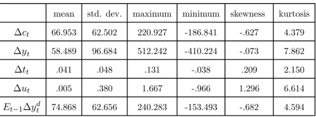
unemployment rate (see e.g. Carroll 1992) and the change in the trend of the personal transfers to GDP ratio (see e.g. Hubbard et al. 1995 and Engen and Gruber 2001). We use the trend change in the transfer rate to reduce the effect of the cyclical component of transfers since this component is strongly correlated with the unemployment rate. For descriptive statistics, a description and the sources of all variables used we refer to table 1 and appendix E.
We write eqs.(21)-(25) as a Gaussian linear state space system with GARCH effects (see Harvey et al. (1992) and Kim and Nelson 1999, chapter 6) where the state vector is
St+1, mt+1=Zt+1St+1+εt+1 (26) St+1 =Tt+1St+πt+1 (27) with εt+1|Ωt ∼N(0, Ht+1) (28) πt+1|Ωt ∼N(0, Qt+1) (29) S0∼N(E(St+1), V(St+1)) (30) where mt+1= h ∆ct+1 ∆yt+1 i0 ,St+1 = h 1 εyt+1 εct+1 εct ψt+1 i0 ,εt+1= h 0 0 i0 , Ht+1= ⎡ ⎣0 0 0 0 ⎤ ⎦,Zt+1= ⎡ ⎣ 1 2γht+1 1 1 θ 1 µ 1 0 0 0 ⎤ ⎦,πt+1 = h 0 εyt+1 εct+1 0 0 i0 ,
Tt+1= ⎡ ⎢ ⎢ ⎢ ⎢ ⎢ ⎢ ⎢ ⎢ ⎢ ⎣ 1 0 0 0 0 0 0 0 0 0 0 0 0 0 0 0 0 1 0 0 (ϕ1+ϕ3xt) 0 0 0 ϕ2 ⎤ ⎥ ⎥ ⎥ ⎥ ⎥ ⎥ ⎥ ⎥ ⎥ ⎦ ,Qt+1= ⎡ ⎢ ⎢ ⎢ ⎢ ⎢ ⎢ ⎢ ⎢ ⎢ ⎣ 0 0 0 0 0 0 ht+1 0 0 0 0 0 σ2c 0 0 0 0 0 0 0 0 0 0 0 0 ⎤ ⎥ ⎥ ⎥ ⎥ ⎥ ⎥ ⎥ ⎥ ⎥ ⎦ ,E(St+1) = ⎡ ⎢ ⎢ ⎢ ⎢ ⎢ ⎢ ⎢ ⎢ ⎢ ⎣ 1 0 0 0 ³ϕ 1+ϕ3x 1−ϕ2 ´ ⎤ ⎥ ⎥ ⎥ ⎥ ⎥ ⎥ ⎥ ⎥ ⎥ ⎦ , diag(V(St+1)) = h 0 ³ δ1 1−δ2−δ3 ´ σ2c σ2c ³σ2xϕ23 1−ϕ2 2 ´i0 , where σ2
c is the variance of εct+1, where x is the sample mean and σ2x is the sample
variance ofxt. Since all states inSt+1are covariance-stationary the initial conditions given
by eq.(30) are non-diffuse. The unconditional means and variances of the states, E(St+1)
and V(St+1), initialize the system.8
The GARCH effects ht+1 complicate the otherwise standard state space framework
sinceht+1 and thusQt+1 is a function of the unobserved stateεyt+1. Harvey et al. (1992)
suggest to replace ht+1 in the system by h∗t+1 =δ1+δ2ε∗yt2+δ3h∗t where the unobserved
ε2yt is replaced by its conditional expectation ε∗yt2=Etε2yt. Note that we can writeEtε2yt=
(Etεyt)2 +Et £
(εyt−Etεyt)2 ¤
.9 From the period t Kalman filter recursions10 we obtain
Etεyt =EtSt[2,1]and Et£(εyt−Etεyt)2¤=VtSt[2,1]. Thus, for given parameter values,
givenh∗
t (which is initialized by the unconditional variance ofεyt+1) and given the Kalman filter output from period t, namely Et(St) and Vt(St), we can calculate h∗t+1 and the
8Note that to apply the method proposed by Harvey et al. (1992) the conditional distributions of the
errors in the state space model are assumed to be Gaussian. Given thatεyt+1 follows a GARCH process, its unconditional distribution is of course not normal (see Hamilton 1994, p.662).
9
Note that the variance of a stochastic variable z can be written as V(z) = E(z2)−(E(z))2. Thus E(z2) =V(z) + (E(z))2.
1 0The Kalmanfilter recursions are (for periodt):
Et(St) =Et−1(St) +Vt−1(St)Zt0F− 1 t (mt−ZtEt−1(St)) Vt(St) =Vt−1(St)−(Vt−1(St)Zt)0 Ft−1(Vt−1(St)Zt)0 0 Et(St+1) =Tt+1Et(St) Vt(St+1) =Tt+1Vt(St)Tt0+1+Qt+1 whereFt=ZtVt−1(St)Zt0+Ht
system matrices Qt+1 and Zt+1. These make it possible to calculate Et(St+1), Vt(St+1)
and Et+1(St+1),Vt+1(St+1), and so on... .
When reporting our results we present graphs of the unobserved component series and of the GARCH series.
4.2
Parameter estimation.
As noted by Harvey et al. (1992) the Kalman filter discussed in the previous section allows us to construct an approximate likelihood function. We use a Bayesian approach to parameter estimation by combining this likelihood with prior parameter information. By maximizing the sum of the sample log likelihood and the log of the prior parame-ter distributions we obtain the mode of the posparame-terior parameparame-ter distribution. More formally, suppose that m = hm0
1 ... m0T i0
(with mt+1 as defined in section 4.1) and
Φ=hθ γ µ δ1 δ2 δ3 ϕ1 ϕ2 ϕ3 σ2c i0
is the parameter vector. Denote the prior parameter density byp(Φ), the (sample) likelihood byp(m|Φ)and the posterior parameter distribution by p(Φ|m). Then the mode of the posterior parameter distribution is given by Φbo = arg max [lnp(Φ|m)] = arg max [lnp(Φ) + lnp(m|Φ)]. The corresponding Hessian-based parameter covariance matrix is obtained asVbo=³h−∂2∂lnΦ∂p(ΦΦ0) −∂2lnp(m∂Φ∂Φ0|Φ)i
Φ=Φeo ´−1
. The mode and Hessian form the basis of the importance sampling approach which is used to obtain (means, variances and percentiles of) posterior parameter distributions. Impor-tance sampling is discussed in the next section.
As far as the priors are concerned we impose priors on the drift parameter µ, on the coefficient of absolute risk aversion γ and on the GARCH parametersδ2 and δ3. A prior
forµ(mean and standard error) is obtained from a preliminary estimation of eq.(22) which gives mean 58 and standard deviation 7. Given the unrestricted range of values µ could take in theory, the prior distribution ofµ is assumed to be normal.
A plausible range of values for the coefficient ofrelativerisk aversion is(0.5,10). Given that the variablect(as defined in appendix F) varies over the sample period from 7500to
21000with a mean of13600a plausible prior forγ(>0) is given by a gamma distribution with mean .0003and standard error.0001.
We also use priors for the parametersδ2 and δ3 because the estimation of a GARCH
model for labour income shocks may be affected by the presence of two outliers in the series for labour income changes. These outliers considerably affect the tails (kurtosis) of the distribution of this series (see figure 1 and table 1). The quadratic form of the GARCH specification tends to extremely magnify outliers in the estimated conditional variance series for income shocks. One way of dealing with this problem is to decrease the weight of the most recent shock ε2yt (i.e. impose a "low" prior on δ2 in the estimation)
and increase the weight of ht (i.e. impose a "high" prior on δ3 in the estimation). We
therefore proceed as follows. Prior estimation of eqs.(22)-(23) separately by maximum likelihood gives a significant estimate for δ2 of about 0.5 and a value for δ3 of almost0.
We therefore first estimate the state space system with a prior for δ2 with mean 0.5(and
standard deviation 0.2) and a prior for δ3 with mean 0.1 (and standard deviation 0.05).
Note that since 0 < δ2, δ3 <1 we use beta distributions as prior distributions. Second,
we check the robustness of our results if we reduce the weight of ε2
yt inht+1 by imposing
a prior for δ2 with mean0.1 (and standard deviation 0.05) and a prior for δ3 with mean
0.5 (and standard deviation0.2).
For the remaining parameters we have no useful prior knowledge so we impose diffuse priors. Note that besides these priors we do not impose parameter restrictions when estimating the mode. Given an appropriate choice of starting values no numerical problems are encountered. Parameter restrictions (e.g stationarity restrictions on the parameters of
theGARCH process) are imposed for importance sampling however. This is discussed in
the next section.
4.3
Importance sampling.
We use importance sampling with sequential updating to obtain posterior parameter distri-butions and posterior states (see Bauwens et al 1999 chapter 3). For givenmthe posterior
state distribution is determined by knowledge of the posterior parameter distribution, so that we can restrict interest to quantities X of the form,
X =
Z Φ
X(Φ)p(Φ|m)dΦ (31)
whereX(Φ)is some function of the parameter vectorΦ. Since the posterior parameter distribution p(Φ|m) is unknown, we useg(Φ|m) as an importance density. Now we write eq.(31) as, X = Z Φ X(Φ)p(Φ|m) g(Φ|m)g(Φ|m)dΦ (32)
which, by using Bayes’ law, can be rewritten as,
X = R ΦX(Φ)z g(Φ, m)g(Φ |m)dΦ R Φzg(Φ, m)g(Φ|m)dΦ = Eg[X(Φ)z g(Φ, m)] Eg[zg(Φ, m)] (33)
where Eg denotes the expectations operator with respect to g(Φ|m) and zg(Φ, m) = p(Φ)p(m|Φ)
g(Φ|m) .
We setg(Φ|m) = N(Φbs, ξVbs) as an importance density where Φbs and Vbs are sequen-tially updated matrices and whereξ is a tuning constant (see Bauwens et al 1999). At the start of the sampling process we set Φbs = Φbo and Vbs =Vbo where Φbo is the mode of the posterior parameter distribution and Vbo is the corresponding Hessian-based covariance
matrix (see section 4.2). By taking draws Φi fori= 1, ..., n from g(Φ|m) we estimateX
by, b X = Pn i=1PX(Φi)zi n i=1zi (34)
wherezi = p(Φg(i)p(mΦi|m)|Φi). Parameter draws fromg(Φ|m) that violate parameter
restric-tions imposed by the model are discarded.11 Posterior parameter means are calculated
from eq.(34) asΦb =
Sn i=1Φizi
Sn
i=1zi . Posterior parameter covariance matrices are then calculated as Vb(Φ|m) = Sn i=1S(Φi)(Φi)0zi n i=1zi − b
ΦΦb0. We then set Φbs = Φb and Vbs = Vb and the sampling
process is repeated. We repeat this sequential sampling process until the coefficient of variation of the weights zi is sufficiently reduced (see Bauwens et al. 1999, chapter 3). Further, the error bounds of the parameter means (see Bauwens et al. 1999 chapter 3, p78) indicate that the approximations of the parameter means obtained through the sampling process are of good quality (only for one parameter is the error bound somewhat high yet it is still below the "critical" threshold reported in Bauwens et al.). Note that in all cases convergence is achieved with 3 or4 updates of the importance density when setting n= 20 000and ξ= 1.2. Thefinal coefficients of variation of the weights and the error bounds of the parameter means are not reported but the results are available from the author upon request.
We further report the means, the variances and percentiles of the final posterior pa-rameter distributions. Note that the 100k% percentile of the posterior parameter distri-bution is Φ[m] taken from the ordered sequence Φ[i] of Φi for which
Sm i=1z[i]
Sn
i=1z[i] ≈
k where
z[i] is the sequence of zi associated to Φ[i]. Note, finally, that the distributions of the posterior states (in particular, state means and state variances) are calculated by running the Kalmanfilter (as described in section 4.1) using the posterior parameter means.
5
Results.
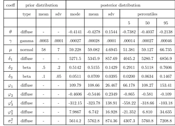
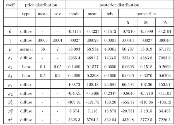
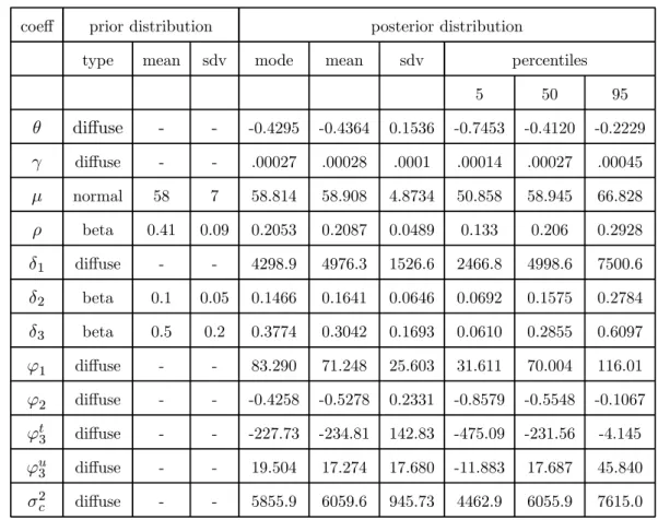
In tables 2 and 3 the estimation results are presented for different priors for δ2 and δ3.
More specifically, we have (δ2, δ3) = (0.5,0.1)in table 2 and (δ2, δ3) = (0.1,0.5) in table
3. Note that for all casesxt contains the first difference in the trend of personal personal
current transfers to GDP ∆tt as well as the change in the unemployment rate ∆ut. The
1 1
We reject draws that violateγ >0,σ2c>0,−0.9< ϕ2<0.9,−0.9< θ <0.9,δ1 >0,δ2>0,δ3>0 andδ2+δ3<1
corresponding parameter vector is ϕ3 =hϕt3 ϕu3
i
. For descriptive statistics, description and sources of these variables we refer to table 1 and appendix E.
From both tables we note first that the modes, means and medians of the posterior distributions of all parameters are of equal magnitude. This is an indication that the distributions are rather symmetric. Note that there is negative autocorrelation in the error term of the consumption function which can be indicative of "noise" in the level of consumption. If we look at the GARCH part of the system we note from table 2 that the posterior means of the parameters δ2and δ3are close to the prior means while the
posterior standard errors are considerably smaller. The data thus puts much weight on the ARCH term. To control whether this is due only to the outliers in labour income we also estimate the system with a high prior forδ3 (table 3). From the estimated conditional
variance series presented in figure 2 we note that the peaks are flattened considerably in the case presented in table 3 where priors are used to shift the weight from the ARCH term to the GARCH term. From a comparison of tables 2 and 3 we note however that that this has little effect on the parameters other than δ1, δ2 and δ3. The reason for
this is that the variation in the conditional variance series is insufficient to explain much of the variation in consumption changes given the estimated values of the risk aversion parameter γ. Aggregate income risk explains not even 1% of the variance of changes in aggregate consumption. Also, given the magnitude of the estimates for γ, the average conditional variance of aggregate income is much too small to be in accordance with the average change in consumption over the sample period. While somewhat disappointing these results are entirely in line with the general presumption that aggregate consumption and income growth are not volatile enough to cause consumption growth under plausible values for risk aversion (see Deaton, 1992 and Gourinchas and Parker, 2001).
Based on our theoretical model, the unobserved component is expected to reflect, at least partially, consumer-specific income uncertainty at the aggregate level. We note,
first, that the constant ϕ1 is positive. Second, the posterior estimates for ϕ2 suggest that there is negative autocorrelation in this component justifying ex post our unobserved components approach. The mean of the posterior distribution of ϕu3 is positive (which is
in accordance with what we expect on a theoretical basis) but its standard error is rather large so that zero values are present between the percentiles 5 and 95 of the distribution. The change in the trend of the personal transfers to GDP ratio, on the other hand, has a negative effect on the change in consumption. From table 2 we can derive that if ∆tt
rises with 25% of its average value then ∆ct+1 decreases with almost 5% of its average
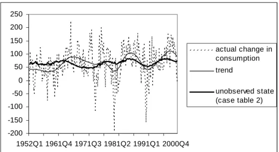
value (see table 1 for descriptive statistics of all variables). In terms of our model this effect seems to indicate that transfers received by consumers diminish consumer-specific uncertainty. This is in line with the literature (see sections 1 and 2). In figure 3 we present the estimated unobserved state ψt with 90% confidence bands. The unobserved component largely follows the change in the trend of the personal transfers to GDP ratio. In figure 4 this component is compared to the trend in the change of consumption. Both trends move together rather closely from the eighties onward suggesting that the trend in the transfers received by consumers may be a good candidate to (partially) explain lower frequency movements in the change in consumption in the US in the second part of the sample. Does our estimated unobserved component coincide with existing results on idiosyncratic income risk ? Storesletten et al. (2004) use both panel and macro data to calculate idiosyncratic risk andfind evidence that it is strongly countercyclical, i.e. higher in recessions. This result is also reported in Parker and Preston (2002). Given the small effect of the change in the unemployment rate (i.e. a proxy for the business cycle) in our results we do not confirm this finding. In the next section we investigate whether this conclusion changes when we extend our model to allow for an effect of income changes on consumption changes.
So, while in the next section we tackle "excess sensitivity" of consumption to current income, in the remainder of this section we discuss "excess smoothness" (see Deaton 1992 for an extensive discussion of both puzzles). From table 1 it is clear that changes in consumption are less volatile than changes in labour income. Yet the finding that labour income is well described by a random walk process suggests that consumption should respond fully to every income shock (i.e our model suggests that consumption changes one-for-one in response to shocks in labour income). This implies that, in theory, consumption
changes should be as volatile as income changes. As this is not the case, the variances of both sides of eq.(21) can only be reconciled if there is negative correlation between some of the variables included as regressors in this equation. We find that there is in fact a significant negative correlation (unreported) between the estimated statesεct+1 andεyt+1.
Since εct+1 contains the period t+ 1shocks in the variance of labour income shocks (ωεt+1
and ωηt+1) and since these shocks enter the consumption equation with a negative sign, a positive correlation between these variance shocks andεyt+1could result in thefinding of
a negative correlation between εct+1 and εyt+1. We can therefore interpret the finding of
negative correlation between the estimated statesεct+1 andεyt+1 as empirical support for
Caballero’s theoretical claim that "excess smoothness" is explainable when income shocks and income variance shocks are positively correlated.
6
Extension: rule-of-thumb consumption.
6.1
Extended speci
fi
cation.
Due to liquidity constraints (see Campbell and Mankiw 1990) or myopia (see Flavin 1985) some consumers may not consume according to the model derived in section 3. We assume that a fractionρ(with0≤ρ≤1) of consumers simply consume their disposable income in each period. To make the extension of our basic model analytically tractable we make the assumption that per capita labour income is identical for both consumer types. Consider the following expression for aggregate (per capita) consumption changes,
∆ct+1=ρ∆ydt+1+ (1−ρ) ∙ κ+1 2γEtε 2 yt+1+ 1 2γB 2E tη2t+1+εyt+1+ωt+1 ¸ (35)
whereyt+1d is aggregate disposable income and whereωt+1= −γ21−δδ22−δ3ωεt+1
−γ2B2 ξ2 1−ξ2−ξ3ω
η
t+1. This equation reduces to eq.(20) if ρ = 0. Consistent with the
model of section 3 the variableyt+1d can be written as the sum of aggregate labour income and aggregate capital income in the economy (i.e aggregate disposable income),
ydt+1 =yt+1+rwtf (36)
wherewft =n−1Pni=1wfitand wherenis the total number of consumers in the economy. From this and given the random walk assumption for yt+1, note that∆yt+1d =Et∆ydt+1+
εyt+1. Therefore we can write,
∆ct+1=ρEt∆yt+1d +εyt+1+ (1−ρ) ∙ κ+1 2γEtε 2 yt+1+ 1 2γB 2E tη2t+1+ωt+1 ¸ (37)
Empirically, eqs.(22), (23), (24) and (25) do not change while eq.(21) is replaced by,
∆ct+1 =
1
2γ(1−ρ)ht+1+ρEt∆y
d
t+1+ψt+1+εyt+1+εct+1 (21’)
where the unobserved component is now defined asψt+1≡(1−ρ)κ+21γ(1−ρ)B2Etη2t+1.
The variable Et∆yt+1d is obtained as the fitted value from a preliminary regression of
per capita disposable income changes on a number of variables that are suggested by Campbell and Mankiw (1990). We refer to appendix E for details. The changes to the state space system are minimal. Only the matrix Zt+1 is different. It is now given by
Zt+1 = ⎡ ⎣ 1 2γ(1−ρ)ht+1+ρEt∆y d t+1 1 1 θ 1 µ 1 0 0 0 ⎤
⎦. There is one additional parameter to be estimated, namely ρ. A Bayesian prior forρ is obtained from Campbell and Mankiw (1990, table 2 row 9). The mean of ρis 0.41 with standard error0.09. The prior distrib-ution is assumed to be a beta distribdistrib-ution.
6.2
Results.
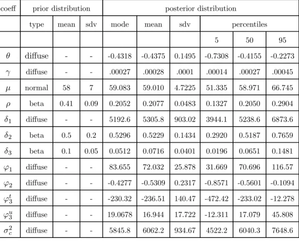
In tables 3 and 4 the results are presented for the estimation of eqs.(21’) and (22)-(25) for different priors for δ2 and δ3. The conclusions drawn for the basic model remain valid
for the extended model. The main difference compared to the results reported for the basic model is that the impact of the trend change of the transfers to GDP ratio, while still negative, is now smaller. Structural increases in the transfer to GDP rate seem to decrease the slope of the consumption path. Based on the model, the channel through which this occurs is through a reduction in consumer-specific income risk. Note again that the unobserved component seems to capture long-run movements of the change in consumption rather than high frequency movements. From looking at the point estimates we note that, compared to the basic case discussed in the previous section, it seems that the change in the unemployment rate now has a larger impact on the unobserved component. Thus it seems that our results are not completely in disagreement with the results of Storesletten et al.(2004) and Parker and Preston (2002). The higher frequency movements in the change of consumption are also explained by the income shock and by the anticipated changes in disposable income. Indeed, note that for the latter regressor the posterior mean ofρis positive with a value of0.2which is lower than what is usually found for this excess sensitivity parameter in the literature. There are a number of potential reasons that can explain why the posterior mean is only half the prior mean. First, the sample period we consider is longer than the one considered by Campbell and Mankiw (1990) since it also contains the nineties. During this period furtherfinancial liberalization may have reduced the number of liquidity constrained consumers leading to lower excess sensitivity (see e.g. Bacchetta and Gerlach 1997). Peersman and Pozzi (2004)find that the excess sensitivity of consumption to anticipated disposable income is0.27in the US for the period 1969-1999. Second, most studies estimate the excess sensitivity parameter whilst improperly omitting income uncertainty terms. As noted also by Hahm and Steigerwald (1999) this produces an upward bias in the excess sensitivity parameter if the income uncertainty term and anticipated disposable income are positively correlated. Hahm and Steigerwald use survey responses to construct a proxy for income uncertainty andfind, for
the US over the period 1981-1994, that income uncertainty increases consumption growth while the excess sensitivity of consumption growth to anticipated disposable income takes on a value of "only" 0.2.
7
Limitations of the approach and concluding remarks.
In the theoretical section of this paper the effect of income risk on consumption changes is decomposed into an aggregate and into a consumer-specific part. Analytical results are obtained under general ARIM A processes for income and GARCH(1,1) processes for income shocks. To obtain these results, like Caballero (1990), we assume that utility is of the CARA type. In Caballero’s paper this type of utility is necessary to obtain a closed form solution for the level of consumption. Since, in this paper, we are mainly interested in consumption changes (that is, in the Euler equation) the use ofCARAutility cannot be justified along these lines. However, it is easy to show thatCARA utility is necessary to make aggregation across consumers possible. Under CARA utility consumption changes at the individual level are linear in the conditional variance of income shocks. Under
CRRA utility individual consumption growth is non-linear in the conditional variance of income shocks (see e.g. Banks et al. 2001). More specifically, under CRRA utility the impact of the conditional variance of income shocks on individual consumption growth varies inversely with the individual-specific wealth level. This multiplicative structure makes aggregation difficult. Avoiding these problems by using CARA utility instead of
CRRA utility comes at a price however. The fact that under CARA utility the wealth level does not enter the Euler equation contradicts Carroll’s (1992) model of buffer-stock savers. In Carroll’s model (which uses CRRA preferences) consumption growth is faster for households with low wealth (all other things equal) because they are building up a buffer against income shocks. An important implication of Carroll’s model is that this mechanism gives a "precaution-based" explanation for the observed "excess sensitivity" of consumption to lagged / predicted income. He argues that when wealth is left out of the Euler equation the finding that lagged or predicted income growth positively affects
consumption growth can be explained by noting that low-wealth periods may coincide with rapid income growth periods (e.g. the periods of fastest income growth might be the early stages of a recovery when wealth is low because buffer stocks have been depleted during the downturn). The implication for our results is then that by using CARAutility wealth is omitted from the Euler equation and observed "excess sensitivity" (as discussed in section 6) can partially12 be caused by this omission. Basically the use ofCARAutility thus implies that the "excess sensitivity" parameterρneed not be unrelated to precaution. While the estimates wefind forρare lower than those found in cases where no time-varying income uncertainty terms enter the Euler equation (see section 6) they may still be too high because of the fact that, under CARA utility, income uncertainty is not interacted with wealth.
Another assumption imposed to derive the theoretical results is the constancy of the real interest rate and its equality to the rate of time preference (contrary to the CARA
utility assumption this assumption is not strictly necessary to derive the model) . This implies that intertemporal substitution effects caused by the (anticipated) interest rate are ruled out. While there is plenty of evidence that the ex ante real interest rate has no impact on consumption growth (see Hall 1988, Campbell and Mankiw 1990 or Ludvigson 1999 for more recent evidence) it is not clear whether this also holds when time-varying income uncertainty is taken into account. Parker and Preston (2002) shed some light on this issue by decomposing the predictable part of consumption growth into a part related to intertemporal substitution, a part reflecting preferences and a part due to incomplete markets (i.e. precaution and liquidity constraints). Theyfind that there is a strong positive correlation between the incomplete markets component and the interest rate component. An implication of their finding is that adding a precautionary component to a regression of consumption growth on the anticipated real interest rate will tend to reduce rather than augment the effect of the real interest rate. Since the existing evidence suggests that this
1 2
We say "partially" because there is no evidence that the "buffer stock" model can by itself explain the magnitude of the observed "excess sensitivity" of aggregate consumption to income (see Ludvigson and Michaelides 2001)
effect is already small when precaution is not taken into account the restriction of zero intertemporal substitution in the presence of incomplete markets seems reasonable.
Empirically, the results of the GARCH estimation seem to confirm the general pre-sumption (see e.g. Gourinchas and Parker 2001) that aggregate income growth is not volatile enough to have a significant impact on consumption growth given realistic esti-mates for the coefficient of risk aversion. While aggregate income risk seems to have no impact on changes in consumption this is not so for the unobserved component which, according to the model, should reflect idiosyncratic risk at the aggregate level. The main problem here is of course that the unobserved component is a catch-all component. It may reflect idiosyncratic income uncertainty but it can also capture other components not in-cluded in the regression. First, the estimated constant in the unobserved component gives no information on the magnitude of idiosyncratic risk since it cannot be distinguished from the average change in consumption which may reflect components not related to risk. Sec-ond, the (negative) autocorrelation found in the unobserved component in our regression results may be due to idiosyncratic risk (i.e. idiosyncratic risk not driven by transfers and unemployment) but could as well reflect omitted variables that are unrelated to idiosyn-cratic risk. Besides the factors included in our estimations and besides the real interest rate we note that predictable consumption changes could be driven by nonseparabilities in the utility function. Examples are situations in which the marginal utility of consumption of non-durables and services is driven by durable consumption, by lagged consumption (habit formation) or by government consumption. While there is little evidence that these factors have an impact on consumption growth when income growth is added as a regressor (see e.g Campbell and Mankiw 1990), as in the case of the real interest rate, it is not clear whether this conclusion remains valid when time-varying income uncertainty is taken into account. The decomposition of Parker and Preston suggests that there is negative correla-tion between the component of predictable consumpcorrela-tion growth related to precaucorrela-tion and the component related to preference shifts (which captures nonseparabilities in the utility function). An implication is then that the relevance of nonseparabilities (which are not taken into account in this paper) to explain consumption growth may be larger when a
precautionary term is added to the regression. When interpreting the results of this paper it is important to keep this caveat in mind.
References
Attanasio, O.(1999): “Consumption,” inHandbook of Macroeconomics, ed. by J. Taylor,
andM. Woodford, vol. 1, chap. 11. Elsevier Science.
Bacchetta, P., andS. Gerlach(1997): “Consumption and Credit Constraints:
Inter-national Evidence,”Journal of Monetary Economics, 40, 207—238.
Banks, J., R. Blundell, and A. Brugiavini (2001): “Risk pooling, Precautionary
saving and Consumption growth,”Review of Economic Studies, 68, 757—779.
Barsky, R., N. Mankiw,andS. Zeldes(1986): “Ricardian consumers with Keynesian
propensities,”American Economic Review, 76(4), 676—691.
Bauwens, L., M. Lubrano, and J. Richard (1999): Bayesian inference in dynamic
econometric models. Oxford University Press.
Browning, M., and A. Lusardi(1996): “Household saving: micro theories and micro
facts,”Journal of Economic Literature, 34, 1797—1855.
Caballero, R. (1990): “Consumption puzzles and Precautionary savings,” Journal of
Monetary Economics, 25, 113—136.
Campbell, J., andN. Mankiw(1990): “Permanent Income, Current Income and
Con-sumption,”Journal of Business and Economic Statistics, 8, 265—279.
Carroll, C.(1992): “The buffer-stock theory of saving: some macroeconomic evidence,”
Brookings Papers on Economic Activity, 2, 61—156.
(1994): “How does future income affect current consumption ?,”Quarterly Jour-nal of Economics, pp. 111—147.
Carroll, C., and A. Samwick (1998): “How important is precautionary saving ?,” Review of Economics and Statistics, 80(3), 410—19.
Dardanoni, V. (1991): “Precautionary savings under income uncertainty: a
cross-sectional analysis,”Applied Economics, 23, 153—160.
Deaton, A. (1991): “Savings and liquidity constraints,” Econometrica, 59, 1221—1248.
(1992): Understanding Consumption. Oxford University Press.
Demery, D., and N. Duck(2000): “Incomplete Information and the time series
behav-iour of Consumption,”Journal of Applied Econometrics, 15, 355—366.
Dreze, J., and F. Modigliani (1972): “Consumption decisions under uncertainty,”
Journal of Economics Theory, 5, 308—335.
Dynan, K. (1993): “How prudent are consumers ?,” Journal of Political Economy, 101,
1104—1113.
Engen, E., and J. Gruber (2001): “Unemployment insurance and precautionary
sav-ing,”Journal of Monetary Economics, 47, 545—579.
Feldstein, M. (1972): “Social security, induced retirement and aggregate capital
accu-mulation,”Journal of Political Economy, 82, 905—926.
Flavin, M. (1985): “Excess Sensitivity of Consumption to Current Income: Liquidity
Constraints or Myopia?,”Canadian Journal of Economics, 38, 117—136.
Gourinchas, P., and J. Parker (2001): “The empirical importance of precautionary
saving,”American Economic Review, 91(2), 406—12.
Guiso, L., T. Jappelli, and D. Terlizzese (1992): “Earnings uncertainty and
pre-cautionary savings,”Journal of Monetary Economics, 30, 307—337.
Hahm, J., and D. Steigerwald(1999): “Consumption adjustment under time-varying
Hall, R. (1988): “Intertemporal Substitution in Consumption,” Journal of Political Economy, 96.
Hamilton, J.(1994): Time Series Analysis. Princeton University Press.
Harvey, A., E. Ruiz, and E. Sentana (1992): “Unobserved component time series
models with ARCH disturbances,”Journal of Econometrics, 52, 129—157.
Hubbard, R. G., J. Skinner, andS. Zeldes(1995): “Precautionary saving and social
insurance,”Journal of Political Economy, 103, 360—399.
Kennickell, A., and A. Lusardi (2001): “Is the Precautionary Saving Motive really
important ?,” .
Kim, C., andC. Nelson(1999): State-space models with regime switching: classical and
Gibbs-sampling approaches with applications. MIT Press.
Kimball, M.(1990): “Precautionary saving in the small and in the large,”Econometrica,
58, 53—73.
Lettau, M., and S. Ludvigson(2001): “Consumption, aggregate wealth and expected
stock returns,”Journal of Finance, 56, 815—849.
Ludvigson, S. (1999): “Consumption and Credit: A Model of Time-Varying Liquidity
Constraints,”Review of Economics and Statistics, 81(3), 434—447.
Ludvigson, S., and A. Michaelides (2001): “Does Buffer-Stock Saving Explain the
Smoothness and Excess Sensitivity of Consumption,” American Economic Review, 91(3), 631—647.
Parker, J., and B. Preston(2002): “Precautionary Savings and Consumption
Fluc-tuations,”NBER Working Paper, (9196).
Peersman, G., and L.Pozzi(2004): “Determinants of consumption smoothing,”
Skinner, J. (1988): “Risky income, life cycle consumption and precautionary savings,” Journal of Monetary Economics, 22, 237—255.
Storesletten, K., C. Telmer, and A. Yaron (2004): “Cyclical Dynamics in
Idio-syncratic Labor Market Risk,”Journal of Political Economy, 112(3), 695—717.
Wilson, B. (1998): “The aggregate existence of precautionary savings: time series
ev-idence from expenditures on nondurable and durable goods,” Journal of Macroeco-nomics, 20, 309—323.
Zeldes, S. (1989): “Optimal consumption with stochastic income: deviations from
cer-tainty equivalence,”Quarterly Journal of Economics, 104, 275—298.
Appendix A: derivation of eq.(2).
We take a second-order Taylor expansion of e−γ∆cit+1 around E
it∆cit+1 which gives the
result (after taking expectations),
Eite−γ∆cit+1 =e−γEit∆cit+1
∙ 1 +γ 2 2 Eit(cit+1−Eitcit+1) 2 ¸ (A1)
Substituting this into eq.(1) and then taking logs gives, after some rearrangements, eq.(2) in the text.
Appendix B: derivation of eq.(12).
We write eq.(2) for period t+j as,
cit+j =cit+j−1+
1
2γEit+j−1ε
2
Writing eq.(B1) for periodt+j−1, substituting this into eq.(B1) and re-iterating until periodt gives, cit+j =cit+ j X k=1 εcit+k+ j X k=1 γ 2Eit+k−1ε 2 cit+k (B2)
Eq.(12) is obtained by adding to and subtracting from the RHS of eq.(B2) the term Pj k=1 γ 2Eitε 2 cit+k.
Appendix C: derivation of eq.(17).
First, using the assumption that the errors εyt+1, ηit+1, ωεt+1 and ω η
it+1 are mutually
uncorrelated and that ωεt+1 and ωηit+1 have variances σ2
ωε and σ2ωη respectively we can,
using eq.(16), writeEit+k−1ε2cit+k=Eit+k−1 ¡
π1εyt+k+π2ηit+k+π3ωεt+k+π4ωηit+k ¢2
=
π21Eit+k−1ε2yt+k+π22Eit+k−1η2it+k+π23σ2ωε+π24σ2ωη. Similarly we can writeEitε2cit+k=
π21Eitε2yt+k+π22Eitηit+k2 +π23σ2ωε+π24σ2ωη. After subtracting the second result from the first we obtain
Eit+k−1ε2cit+k−Eitε2cit+k =π21 ¡
Eit+k−1ε2yt+k−Eitε2yt+k ¢
+π22¡Eit+k−1η2it+k−Eitη2it+k ¢ (C1)
Second, wefind expressions forEit+k−1ε2yt+k−Eitε2yt+kandEit+k−1η2it+k−Eitη2it+k. We
only present the derivation of Eit+k−1ε2yt+k−Eitε2yt+k as the derivation ofEit+k−1η2it+k−
Eitη2it+kis completely identical. Note that we can write eq.(5) asε2yt+1=δ1+(δ2+δ3)ε2yt−
δ3ωεt+ωεt+1 and for periodt+kasε2yt+k =δ1+ (δ2+δ3)ε2yt+k−1−δ3ωεt+k−1+ωεt+k. After
ε2yt+k = δ1 ³ 1 + (δ2+δ3) + (δ2+δ3)2+...+ (δ2+δ3)k−1 ´ (C2) +ωεt+k+ωεt+k−1(δ2+δ3)0δ2+ωεt+k−2(δ2+δ3)1δ2 +ωεt+k−3(δ2+δ3)2δ2+...+ωεt+1(δ2+δ3)k−2δ2 −ωεt(δ2+δ3)k−1δ3+ (δ2+δ3)kε2yt
Taking expectations of eq.(38) with respect to info set Ωit+k−1 and info set Ωit and
subtracting the last result from thefirst we obtain,
Eit+k−1ε2yt+k−Eitε2yt+k= k−1 X h=1
δ2(δ2+δ3)k−1−hωεt+h (C3)
Similarly we can write
Eit+k−1η2it+k−Eitη2it+k= k−1 X h=1
ξ2(ξ2+ξ3)k−1−hωηit+h (C4)
Using eqs.(C3) and (C4) into eq.(C1) and the result into eq.(15) we can write,
∞ X j=1 αj{(j >2) j X k=2 γ 2π 2 1 k−1 X h=1 δ2(δ2+δ3)k−1−hωεt+h+(j >2) j X k=2 γ 2π 2 2 k−1 X h=1 ξ2(ξ2+ξ3)k−1−hωηit+h + j X k=1 εcit+k− j X k=1 A∗j−kεyt+k− j X k=1 Bj∗−kηit+k}= 0 (C5)
This condition should be satisfied period-by-period since εyt+1, ηit+1, ωεt+1, ω η it+1and