Facultad de Ciencias Económicas y Empresariales
TRABAJO FIN DE GRADO EN
PROGRAMA INTERNACIONAL DE ADMINISTRACIÓN Y DIRECCIÓN DE EMPRESAS
THE EFFECTS OF THE ECB’S QUANTITATIVE EASING ON LENDING, DEPOSITS, AND FINANCIAL STABILITY.
Ane Bakiakoa Pedrosa
Pamplona-Iruña 16 de mayo de 2019
DIRECTOR: José Manuel Mansilla Fernández Módulo: Finanzas
2
INDEX
1. INTRODUCTION………5
2. LITERATURE REVIEW……….7
2.1. The transmission channels of the Monetary Policy……….9
3. MONETARY POLICY IN EUROPE: OVERVIEW………...13
3.1 Monetary decisions in a nutshell………....16
4 MONETARY AGGREGATES AND ITS COUNTERPARTS……….……...18
5 WHAT HAS ECB DONE COMPARED TO ENGLAND AND USA……....21
6 DATA AND EMPIRICAL APPROACH………25
6.1 Data……….….….25
6.2 Empirical approach………....26
6.3 Hypothesis……….…27
7. EMPIRICAL RESULTS………..27
7.1 The baseline regression………...31
7.1.1 The effects of QE on credit supply………...….31
7.1.2 The effects of QE on bank market concentration (lending and deposits).…..33
7.1.3 The effects of QE on financial stability………...37
8 CONCLUSIONS………..….39
9 REFERENCES……….………...41
3
INDEX OF DIAGRAM
Diagram 1: Timeline of Central Bank’s Unconventional Monetary Policy decisions ... 21 INDEX OF FIGURES
Figure 1: ECB decisions regarding QE ... 17 Figure 2: Monetary aggregates (annual growth, seasonally adjusted) ... 20 INDEX OF TABLES
Table 1: Shortage of the consolidated balance sheet of Monetary Financial Institutions elaborated with M3 and its counterparts... 19 Table 2: First round of bond purchases under the QE program by the Bank of England.. 22 Table 3: Decisions taken by the FED regarding QE programme. ... 24 Table 4: Descriptive Statistics ... 28 Table 5: Parametric tests for the comparison of means for the pre-crisis (2002Q1-2007Q2), crisis period (2007Q3-2015Q1), and the QE period (2015Q2-2016Q4). ... 29 Table 6: The effects of the crisis and the unconventional monetary policy on lending supply from 2002Q1 to 2016Q4. ... 32 Table 7: The effects of the crisis and the unconventional monetary policy on
HHI_LOANSit from 2002Q1 to 2016Q4. ... 34 Table 8: The effects of the crisis and the unconventional monetary policy on HHI_DEPO from 2002Q1 to 2016Q4 ... 35 Table 9: The effects of the crisis and the unconventional monetary policy on financial stability from 2002Q1 to 2016Q4. ... 38
4
The Effects of the ECB’s Quantitative Easing on
Lending, Deposits, and Financial Stability
Ane Bakaikoa Pedrosa
Abstract
This article analyses the effect of the ECB s Quantitative Easing (QE hereafter) programme on lending supply, collection of deposits and financial stability in the Euro Area banking markets. For this purpose, a panel data regression is used covering the time span between 2002 and 2016. The results suggest that although the QE did not help to increase lending supply, it contributed to concentrate the Euro Area lending and deposits markets. Furthermore, the results of this study also suggest that the QE, which implies negative interest rates, contributed to the reduction of financial stability through a reduction in bank's profitability.
Keywords: Quantitative Easing, bank lending, deposits, financial stability, monetary policy. JEL Classification: E52 G01 G21 G28
Resumen
Este artículo analiza los efectos del programa de expansión cuantitativa (QE por sus siglas en inglés) implementado por el Banco Central Europeo desde marzo de 2015 hasta la actualidad. Para ello, se ha hecho uso de una regresión con datos de panel que cubre el periodo entre 2002 y 2016. Los resultados de este estudio sugieren que, aunque el programa de QE no ha impactado sobre la oferta de crédito, ha contribuido a concentrar los mercados de crédito y de depósitos. Además, los resultados de este estudio sugieren que la QE, que implica tipos de interés negativos, ha contribuido a reducir la estabilidad del sistema bancario debido a la reducción de rentabilidad de los bancos.
Palabras clave: Expansión cuantitativa Crédito bancario, depósitos bancarios, estabilidad financiera, política monetaria.
Clasificación JEL: E52 G01 G21 G28
Advisor: José Manuel Mansilla Fernández Departamento de Gestión de Empresas
5 “The problem with Quantitative Easing is that it works in practice, but it doesn’t work in theory.” –Ben Bernanke, January 2014.
1. INTRODUCTION
The financial crisis of 2007-2008 has introduced new monetary policy measures leading to debates among economists regarding their macroeconomic effects. The market fragmented due to the Sovereign Debt Crisis and the interbank lending stopped. These circumstances broke the price stability that the European Central Bank (ECB hereafter) has the mandate to maintain after the Treaty of Maastricht in 1992. (Treaty on European Union. The Official Journal of the European Community, page 68). Central banks started reducing policy interest rates sharply to provide further stimulus, including large-scale purchases to raise public and private asset prices, and forward guidance to communicate about future directions of monetary policy (Molyneux et al., 2019). The effectiveness of these unconventional measures of monetary policy is currently under a lively debate without a clear consensus. However, since 2012, six European economies and Japan introduced negative interest rates policies. Central banks use these unconventional measures when traditional monetary policy instruments cannot longer be applied (Smaghi B., 2009). Therefore, unconventional monetary policies are aimed at addressing weak macroeconomic performances and supporting financial intermediaries. Nonetheless, there could exist problems with these measures when the interest rates remain low for too long.1 Accurately, the first question posed by this paper is: Can it be proven that unconventional monetary policy may increase banks’ lending supply? And what is more: Can unconventional monetary policy affect concentration in banking markets? This paper focuses on the Asset Purchase Programme (APP hereafter) implemented by the ECB from March 2015 onwards which was aimed at unfreeze the Euro Area financial markets. With this program, the central bank buys assets with long maturities to public and private sectors in order to provide the banking system with a provision of liquidity. By means of the purchases, the price of these assets increase and the interest rates decrease, facilitating the borrowing and the repayment of them by investors and firms. As a consequence, consumption and investment increase pushing up employment and economic growth. When
1 Beaupain and Durré (2015) conducted a study regarding the excess liquidity and the money market and concluded, on the one hand, that the relation between the excess liquidity and the dynamics of the interbank market started with the implementation of the FRFA; on the other hand, they stated that the FRFA had hoard the market. In the second phase of the crisis, the Sovereign Debt Crisis took place so the duty of the ECB was focused on addressing the market and reducing differences in the financial conditions of businesses and households.
6 the process ends, the Central Bank’s objective of maintaining an inflation rate below, but close to 2%, over the medium term is met (ECB, 2018). In specific terms, the third research question could be formulated as follows: Can the unvencional monetary policy increase financial stability? In other words, the effectiveness of the European Quantitative Easing (QE hereafter) is analyzed in order to shed a light to the unconventional measures and their subsequent international spillovers and side effects.
The empirical analysis uses a panel data from Bankscope and Orbis Bank Focus (Bureau van Dijk) containing 191 Eurozone banks for the period 2002 to 2016. The panel is completed with macroeconomic data obtained from Thomson Reuters Datastream. As for the variables used in this study, lending supply is calculated as the loans to customers to total assets ratio (e.g., Chiesa and Mansilla-Fernández, 2018a, b). We proxy for banking concentration by using the Herfindahl-Hirschman Index for lending and deposit markets (Carbó and Rodríguez, 2007; Carbó et al., 2009). Lastly, financial stability is calculated using the Z-score indicator as employed in the financial literature to assess the inverse probability of banks’ default (Laeven and Levine, 2009; Schaeck et al., 2012; Liu et al., 2013; Köhler, 2015).
I implement these indicators by using the difference-in-differences (DID hereafter) method to assess whether the QE contributed to the recovery of lending supply and financial stability. This study contributes to the current literature by shedding a light to the effects of unconventional monetary policy measures on the performance of banking markets. In line with recent studies (Molyneux et al., 2019), I find that the ECB’s QE did not help to increase lending supply. This result might be driven by reductions in the demand for loans due to the deleveraging of the real sector and adverse macroeconomic conditions. However, we find that lending and deposits markets become relatively more concentrated after the implementation of the QE. Contrary to our expectations, financial stability diminished following the QE due to reductions in banks’ interest margins as a consequence of negative interest rates.
The remainder of the paper is organized in eight sections. Section two discusses the related literature. Section three summarizes the monetary decisions taken by the ECB. Section four explains the monetary aggregates and its counterparts. Section five relates the ECB with the Central Banks of United Kingdom and United States. Section six presents the hypotheses, defines the database and describes the empirical model along with the variables employed. Section seven provides a discussion of the results, and section eight closes the paper with a concluding remark.
7
2. LITERATURE REVIEW
Keyne’s (1936) seminar paper advocates that the expansionary monetary policy ceases to be effective in a liquidity trap; argument that has been proved to be misled with the QE adopted by the Japanese monetary authorities in March 2001.
The 2008 financial crisis changed the role of central banks due to the dependency of financial stability on market behavior. According to Giménez Roche and Janson (2019), central banks switched from acting as lenders of last resort, to market-makers of last resort. The impact of this change resulted in the application of unconventional monetary policies, also known as QE, as a consequence of open market operations beyond the interbank money market. Under the lenders of last resort role, the central bank offers loans to banks that are in a risky situation and guarantees a safety degree to the customers who want to withdraw their funds. As a result of the crisis, the central bank’s role went beyond the interbank money market and had to intervene in other markets assuming its role of market-makers of last resort (Mehrling, 2011).
In this paper, I run a placebo test by applying unconventional monetary policy measures before the crisis to prove the robustness of my results. Although the QE can prevent a collapse, it is not designed to promote long-term growth (Lombardi et al., 2018). Besides, unconventional measures are considered a treatment for the financial break that the world economy was living, so it makes no sense to use QE in times when conventional monetary policy can be applied.
Unconventional monetary policies differ across countries and each central bank takes its own decisions on how to maintain prices stable and boost economic growth. First, the ECB generated electronic funds to increase bank lending and consumer spending, and afterwards, it introduced inflation targets and variables that contributed to the stimulation of the economy. Likewise, the Federal Reserve (FED hereafter) employed three Large Scale Asset Purchase (LSAPs) programs, i.e. QE1, QE2 and QE3, with different efficiency levels. Fratzscher (2018) examined the effects of the QE on global portfolio flows and stated that QE12 increased the procyclicality of flows to the non-US nations resulting in a portfolio rebalancing towards the assets of US. He added that instead, the QE2 and the QE33 resulted in a portfolio rebalancing towards the assets of non-US nations. To the best of my
2 QE1 was launched by the FED on October 2008 and ended on March 2010.
8 knowledge, economic literature has search for the relationship between US and Euro area’s interest rates. In this sense, Meegan, Corbet and Larkin (2018) used a market model framework, with a nested EGARCH specification, to test for spillover effects and volatility contagion.
Although the European crisis resulted in a structural break in interest rates, sovereign bonds and lending, there is no evidence that the FED’s asset purchases did have a significant impact on the trans-Atlantic interest rate relationship with Europe (Belke et al., 2017). Indeed, the QE2 matches in the time period line, but it has been the less effective QE program by the FED, so there is little evidence that it has any impact on the structural break between US and European long-term interest rates.
As for the ECB’s decisions, the QE1 was implemented in the middle of the crisis having large effects on providing liquidity. However, the QE2 was relatively more anticipated by market participants than the QE1. In sum, I base my analysis on the idea that the QE1 was successful in UK and USA; but also, on the idea that that taking into account the cost-benefit analysis, it cannot be assure that QE2 was successful too. However, recent studies differs in the effectiveness of the QE, comparing the Euro Area and the UK and USA, due to the configuration of their financial systems. On the one hand, the Euro Area financial system is bank based, which relies more on banks to transmit changes in macroeconomic interest rates to the real economy. On the other hand, the UK and USA financial systems are market based, which smooths the access to markets to borrowers to obtain funds. These differences in financial architecture between the continental and the Anglo-Saxon financial systems make us think that the QE could be comparatively less effective in the Euro Area than in the UK and USA. In this regard, Gern et al. (2015) identify two main problematic approaches evaluating QE effects: The time series analysis and the announcement model. They assumed that markets were efficient in the sense that all the effects on yields occurred when market participants updated their expectations and not when actual purchases took place.
I took into account the existing heterogeneity within the Euro Area, which explains why the effects on bank lending are not the same in Germany and in Spain (or similarly, in periphery and core countries). This heterogeneity is reflected in the banking system in terms of agency costs, expected investment and net worth. Before 1999, the transmission of monetary policy did not seem highly heterogeneous across Germany and Spain (Ehrmann et al., 2003), so I will deepen in this matter to explain which variables are the one that has changed.
9 In this line, I attempt to analyze the existence of financial spillovers. Indeed, Hanisch (2019) has empirically proved that contractionary US monetary policy may have generated short-term expansionary spillover effects via trade and financial channels. The spillovers were bigger before the adoption of the euro due to the lack of homogeneity between Euro Area members. As global markets became more integrated, the role of credit market increased and the sensitivity to foreign monetary policy shocks decreased. Note that not every country within the Euro Area responded in the same way. In Germany, the convergence process entailed lower output responses, while in Spain it entailed higher output responses. At any rate, the integration has led to an increased in the confidence showed by investors resulting in a decreased in the risk premia.
2.1. The transmission channels of the Monetary Policy
Previous studies analyzed the transmission channels of the QE with a common and shared objective: to explain the different effects of the central bank`s APP. The studies agree that the aim of the policy is to restore financial stability to levels prior to the crisis. The number of existing channels have been an issue since some authors talked only about two: portfolio-rebalancing channel and signaling channel (Cecioni M. et al., 2011), while others, preferred to talked about several more, even if the most widely analyzed is the portfolio-rebalancing channel (see Altavilla et al., 2015, for the Euro Area; Joyce et al., 2011 for the UK; and D’Amico et al., 2012, for the US).
However, the nexus between asset purchases and their prices and yields, leads to an open debate between economists. They agree on the issue that asset prices and yields were mainly affected by the reduction of risk premia through portfolio rebalancing effect. Joyce and Tong (2012) studied the impact of BoE’s APP and concluded that it affects via local supply effects, since the yields purchased fell by a higher amount, and via the duration risk effects, since longer maturity bonds were the ones that suffered larger yield falls.
In the case of USA, D’Amico et. al (2013) found that the first two rounds of QE impacted through the scarcity and duration channels. Contrary to this view, Krishnamurthy and Vissing-Jorgensen (2011) did not find empirical evidence regarding the duration channel. They argued that the QE applied by the FED had an impact through the safety channel. This channel predicts that QE lowers the yields on very safe assets relative to less safe assets, increasing safety premium. It reflects a deviation of safety spread between assets depending on the market demand. They made a regression to test whether there was any impact through
10 the liquidity channel and found positive results. Indeed, this channel predicts a benefit for investors to sell their assets in regards to the increase in yields that the most liquid assets (treasury bonds) experienced in relation to the less liquid ones (agency bonds) after the QE. The prepayment risk premium channel appeared in the first phase of the QE of the United States but there is no evidence about its presence on the second phase. Mortage-Backed securities carried heavy prepayment risk. When the government buys these securities, it reduces the prepayment risk. (Gabaix et al., 2007).
Importantly, Altavilla et al. (2015) show that the policy asset is not limited to times of financial market stress, but the strength of the channels of transmission might have differed across risk and liquidity regimes. Accurately, the bank-lending channel suggests that when the ECB buys private sector assets, their prices are driven up and consequently, it encourages banks to make more loans as they lowered bank lending rates for firms and households. Furthermore, when banks are not able to substitute liabilities with funds, either because they are in a personal risky situation or because a global crisis, the effect is turned into the asset side of their balance sheet. The bank lending channel is, thus, the consequence of bank’s funding shocks.
Before listing the channels through with monetary policy achieves its results, I will define a channel that breaks in times of QE: The interest rate channel. Regarding the negative deposit facility rate, banks find it difficult to mitigate the adverse effects that negative interest rates have on their net interest margins, and consequently, on their profitability (Bernoth and De Haas, 2018). Brunnermeier and Koby (2017) argued that if interest rates fell below reversal rates levels, bank’s capital and profitability could be negatively affected and eventually, restrict credit supply.
The foremost financial literature is growing towards the analysis of the portfolio rebalancing channel following the sovereign debt crisis and the ECB’s APP. In this regard, when the ECB buys private and public sector assets, investors change their portfolio holdings by investing in other assets. Such action, lowers funding costs, and stimulates investment and consumption. European banks substituted risky assets investments for excess liquidity (from liquid assets to credit supply) when the ECB set negative interest rates. In other words, they change the composition of their portfolios turning from lower yield assets to higher yield assets, thus, flattening the yield curve (Bottero et. al, 2019).
11 In the case of investors, they rebalance their portfolio buying similar assets, inducing trading, since the existing base money and the assets purchased through QE are not perfect substitutes.
Through the signaling channel, asset purchases signal to the market that the central bank will keep key interest rates low for an extended period of time. This, in turn, modifies market participants future expectations. The fact that increasing interest rates would mostly harm the Central Bank`s purchased assets increases the credibility of their actions. Eggertson and Woodford (2003) argue that if such policy remains even after the economy recovers, the QE will be beneficial, since volatility and uncertainty in the market regarding future interest rates is reduced.
The duration risk channel which appeared in studies for the USA and UK, is reflected by a premium in bond yields due to the impact that a change in the interest policy may have in long-term bonds. It also appeared in the Euro Area when the forward guidance and the QE announcement reduced rates reaching in March 2015 to a historical low, increasing the average maturity of issued government debt securities (Valiante D., 2017).
In this regard, the important role of foreign banks should be highlighted since they have expanded to emerging markets reaching for higher yields, and thus, creating a credit boom. It is, therefore, possible to identify two more transmission channels: the international credit channel and the risk-taking channel. Borio and Zhu (2012) used the term “risk-taking channel” to refer to the willingness of market participants to take risks and influence real economy decisions. Internationally, there are evidence about financial spillovers in cross-borders capital flows through the banking sector. Cetorelli and Goldberg (2012a, 2012b) provided direct evidence that global banks managed liquidity on a global scale, actively using cross‐ border internal funding in response to local shocks. Morais et al., (2019) add that local credit supply, was affected by foreign monetary policy shocks through foreign banks.
The Single Supervisory Mechanism and the Single Resolution Mechanism are the responsible for the EU banks supervision. While US banks quickly cleaned up their balance sheets and built up capital after the 2008 financial shock, EU banks are still recovering due to the macroeconomic environment of low interest rate that they are into.
In fact, in September 2018, EU has an excess liquidity of 17% of its GDP held in three different accounts: The current account, the deposit facility for banks account and its fixed-term deposit instrument for certain monetary purposes. In this sense, the most liquid assets
12 that commercial banks can hold are their reserves held at the Central Banks, which can be used to satisfy minimum reserves requirements converted to cash if customers wished to take out their bank deposits, and transferred to other banks to settle payments. In terms of converting banks’ reserves to cash, one might expect that as a result of low and even negative deposit rates, cash holdings can go up. Nevertheless, according to Darvas and Pichler (2018) when interest rates are low globally, people and companies outside the Euro Area might also hold more euro cash.
The sensitivity that the banking sector has demonstrated until now has been the aim of study of various authors. Different ideas have arisen complicating the research, so I take out some controversial facts to ease the understanding. The effects that monetary policy has on banks will, ultimately, determinate the influence of the sovereign debt.
Bank capital and credit supply are affected by the regulatory framework. If the economy experiences an expansionary phase, banks take more credit risk improving their liquidity and net wealth. Indeed, by making risk-free assets less attractive, low interest rates may lead financial intermediaries to make riskier investments. On the contrary, if the economy is in a contractionary phase, banks have to bear more costs, thus, bank lending decrease and so does the risk-taking (Popov and Van Horen, 2013). The econometric analysis by Demiralp et al., (2017) concluded that the negative ECB deposit interest rate led to more lending by banks. The negative ECB deposit rate along with asset purchases might compensate for each other in the banks’ profits (Blot and Hubert, 2016).
Other studies have focused on analyzing how the UMP has affected the bank credit and concluded that in general they have a positive impact on credit that takes place 1 or 3 months after its implementation. Money and credit are the two sides of the Central Bank balance sheet in conventional times and are highly correlated. In crisis times, these are no longer correlated and so, this weak link (and the zero lower bound issue) explains the ineffectiveness of the monetary policy after 2008 (Stiglitz, 2016).
Regarding capital flows, it is necessary to associated each phase of the QE with an increase or decrease in net bond and equity inflows. As for European Union countries, the episodes of QE were marked by a relative surge in equity inflows rather than bond inflows (Khatiwada, 2017). Monetary policy, thus, can affect economic activity in the short run, as well as the rate of inflation in the long run.
13 In this paper, I will use these ideas as a base to construct an econometric regression which show the impact of the QE in variables relevant at the banking level with the aim to contribute to the literature that examines the evolution of the financial crisis and the European Sovereign Debt. In this period, starting in 2008, European businesses and economies have suffered a great loss of confidence among the investors due to the liquidity premia. The collapse of financial institutions and the high government debt created the need of a new policy to reach the financial stability that was already lost.
3. MONETARY POLICY IN EUROPE: OVERVIEW
This paper analyses how the unconventional monetary policy applied by the European Central Bank affected lending supply and financial stability of the Euro Area banking sector. In particular, I examine the evolution of the monetary policy starting before the crisis and highlighting the important decisions that the ECB has made through the journey. These decisions brought with them financial spillovers that have allowed us to make comparisons between the US, Japan’s and UK’s QE.
Before the crisis, the ECB provided the banking system with the estimated liquidity needs in a weekly basis via open market operations, the monetary base was exogenously determined by the central bank, and EONIA was set at a positive amount.
In 2007-2008, the advanced economies suffered the biggest financial crisis since the 1930s, followed by a severe post-crisis recession, questioning the adequacy of traditional tools. In January 2009, the former president Jean-Claude Trichet was asked about the liquidity trap, and the measures implemented after this date were called non-standard actions but considered temporary in nature. It was in 2013 when the president Mario Draghi, announced that the policy will remain accommodative for as long as needed. In 2014, the ECB talked for the first time about “unconventional measures” since Zero Lower Bound was making conventional monetary policy ineffective.
After the collapse of the Lehman Brothers, the actions of the ECB were enhanced to provide credit support until it became insufficient and the liquidity demanded was unstable.
14 At that point, in 2008, the ECB decided to establish FRFA4 system to allow the banks to have access to liquidity offsetting any related risk.
In 2008-2009, the real sector decided to turn into cash for safety reasons. The need for liquidity increased the capital flows among countries leading to negative financial spillovers between the advanced countries. Several authors studied the policies and its spillover effects across countries (see Meegan et al., 2018). Excess liquidity started in these years and experienced an annual increased since banks demanded to ease the risks. It reached its maximum in 2012 and went down to almost zero in 2014. Indeed, the cost for holding that liquidity, was higher than the negative interest rate to be paid. Finally, in 2015, regarding the expansion of APP, inflation increased and so did the excess liquidity. As a result of the negative rates, and considering that direct costs are associated to the liquidity that Central Banks held, banks created a strategy to avoid holders to turn massively into cash (Jobst and Lin, 2016).
The ECB announced Long Term Repurchase operations (LTROs), “Main refinancing operations (MRO)” and “Outright Monetary Transactions (OMT) in September 2008, in order to support bank lending and money market activity. The programs were phased out in 2010, but reintroduced later. In May 2009 the ECB announced a Covered Bond Purchase Program under which they purchased €60 billion of private sector bonds. In May 2010 a Securities Market Program was introduced, and later in 2011 until October 2012, a second covered bond purchase program, CBPP2, was launched (ECB, 2011).
Nonetheless, these programs are classified as “Terminated Programs” by the ECB as they were not able to convince the market that there was not risk of default. These policies are not completely similar to the pure the QE since their main target is to restore the banking sector and not the economy as a whole. In this sense, the QE applied by ECB is distinguished from that applied by the Central Bank of Japan, UK, and USA. To face this problem, they introduced alternative measures.
Ben Bernanke, distinguished the unconventional measures applied by the FED from the one applied by the Bank of Japan. He described the approach implemented in the USA as credit easing since it was focused on the mix of loans and securities that it held and on how this composition of assets affected credit conditions for households and businesses, instead
4 Fixed Rate Full Allotment was introduced in every refinancing operations at different maturities. The ECB’s monetary policy during the crisis.
15 of focusing just on the quantity of bank reserves. In this vein, Rodríguez and Carrasco (2016) put in doubt whether ECB measures were a type of QE, and stated that they are not QE in the traditional sense since the expansion in the ECB balance sheet came primarily from increases in the extraordinary longer maturity loans.
The asset purchasing programs were introduced in 2009 as a consequence of the difficult evolution the European financial crisis was experiencing. The ECB had to focus in restoring the whole stability that was being lost in markets other than the banking sector.
When in 2014 ECB introduced a negative deposit interest rate, the banking system was negatively affected throughout the net interest income and the negative profitability (Darvas and Pichler, 2018). Empirical results of Arce et al., (2018) suggested that the affected banks showed lower capital ratios than the no affected banks, making them to assume lower risks. As a result, their net interest income decreased graying them out from the possibility of compensating their losses increasing credit supply.
Finally, in 2015, the Extended Asset Purchase Program was introduced, resembling the purest part that the QE has ever taken in Europe. The program added the purchase of bonds to the ECB’s existing asset purchases portfolio in light of the prolonged low inflation period that Euro Area was living. This fact also facilitated policy makers and economist to make comparisons across borders between the QE applied by USA, UK and Japan, and the one applied by the ECB.
Currently, after almost 4 years of quantitative easing, the ECB has decided to establish an ending point to the net purchases under APP as stated by the president Mario Draghi. However, the ECB will continue reinvesting in full, the principal payments from maturing securities purchased under APP. In order to ensure financial stability and a sustained inflation rate, they will maintain the current level of rates until at least the summer of 2019. In March, the president announced on the one hand, a third TLTRO that will start in September 2019 and end in March 2021, each with a maturity of two years5. The main objective of the operation is to maintain favorable bank lending conditions. On the other hand, the continuity of lending operations at FRFA was announced for as long as necessary. The steps that ECB are making after the end of net purchases and regarding the intention of decreasing the
5 Is not the first time that a speech by the president causes a big commotion, in fact, in July of 2012, when the Euro Area was emerged in the middle of the crisis, Mario Draghi made the famous remark: “Within our mandate, the ECB is ready to do whatever it takes to preserve the euro. And believe me, it will be enough”.
16 reinvestments after the increase of interest rates to positive levels are similar to those made by the FED after the end of their asset purchases under APP (Arce et. al., 2018).
One week later, as I mentioned, the Outright Monetary Transactions were announced aimed at making sure the singleness of the monetary policy. Although it ended up being terminated, it served to decrease the bond yields and preserve investor’s confidence in the market (Altavilla, Giannone, Lenza, 2014)
All in all, the unconventional monetary policy decreased the sovereign credit risk but there is still the need of strong institutions to coordinate economic policy, guarantee competitiveness and encourage sustainable growth as stated by the former Vice president of the ECB, Vítor Constâncio (speech at the FT Banking Summit "Ensuring Future Growth", 2014).
3.1. Monetary policy decisions in a nutshell
The ECB announced the QE in the Euro Area in January 2015 and asset purchases began in March 2015. The plan announced was to buy at least €1.1 trillion of public sector debt and private sector assets between the start of 2015 and September 2016. Now, after almost 4 years of quantitative easing, the ECB has decided to establish an ending point as stated by Mario Draghi in a press-conference following the meeting of the Governing Council of the European Central Bank on 13 December 2018 in Frankfurt: ¨Based on our regular economic and monetary analyses, we decided to keep the key ECB interest rates unchanged. We continue to expect them to remain at their present levels at least through the summer of 2019, and in any case for as long as necessary to ensure the continued sustained convergence of inflation to levels that are below, but close to, 2% over the medium term. Regarding non-standard monetary policy measures, our net purchases under the asset purchase program (APP) will end in December 2018¨.
Figure 1 describes the decisions taken by the ECB regarding asset purchases from March 2015 till December 2018.
17
Figure 1: ECB decisions regarding QE
Source: Author’s own elaboration based on the information retrieve from the European Central Bank.
After the first year of the QE, in March 2016, the ECB lowered the interest on the main refinancing operations and on the marginal lending facility, increased monthly bond purchases (from €60bn to €80bn), include corporate bonds into the list of assets eligible for regular purchases, targeted new long-term loans (TLTRO II), and reiterates forward guidance on borrowing costs.
The ECB decided to reduce purchases to €60 billion in April of 2017. The president of ECB, Mario Draghi, announced in a press conference that the economy was recovering but that a substantial degree of monetary accommodation was needed to get a headline inflation in the medium term.
In June of 2017, regarding the information that has become available since late April, it was confirmed a stronger momentum in the euro area economy, which is projected to expand at a somewhat faster pace than previously expected. It was considered that the risks to the growth outlook were broadly balanced.
In October of 2017, Mario Draghi announced in a press conference held in Frankfurt, that from January 2018 net asset purchases are intended to continue at a monthly pace of €30 billion until the end of September 2018. Also, that the Eurosystem will reinvest the principal payments from maturing securities purchased under the APP for an extended period of time after the end of its net asset purchases to contribute both to favorable liquidity conditions and to an appropriate monetary policy stance. They also decided to continue to
€0 €10.000.000.000 €20.000.000.000 €30.000.000.000 €40.000.000.000 €50.000.000.000 €60.000.000.000 €70.000.000.000 €80.000.000.000 €90.000.000.000 M ar -1 5 Ju n -1 5 Se p -1 5 D ec-1 5 M ar -1 6 Ju n -1 6 Se p -1 6 D ec-1 6 M ar -1 7 Ju n -1 7 Se p -1 7 D ec-1 7 M ar -1 8 Ju n -1 8 Se p -1 8 D ec-1 8
18 conduct the main refinancing operations and three-month longer-term refinancing operations as fixed rate tender procedures with full allotment at least until 2019.
In January 2018, the ECB reduces the monthly pace of its asset purchases to €30 billion euros, and stresses the importance of its reinvestments as a way to support a monetary stimulus. Since the economic expansion has accelerated more than expected and there has been a reduction of economic slack, meaning a balanced equilibrium of the demand relative to what the economy is capable of producing, it has strengthened further the confidence that inflation will converge towards 2%.
In March 2018, the ECB quit from their monetary statement the part where they commit to increase the size of quantitative easing. In front of this, the president of the ECB was questioned in the press conference about this issue and he answered the following: ¨it was a sentence introduced in 2016, when we cut our monthly purchases from €80 to €60 billion. Thinking about that, you can just figure out, how different the situation was at that time. The sentence says: if the outlook becomes less favorable or if financial conditions become inconsistent with further progress towards a sustained adjustment in the path of inflation, we stand ready to increase the asset purchase program in terms of size and/or duration. So, what we did was to remove the explicit reference to the likelihood of an increase in the pace of purchases in the near future¨.
In June 2018, the ECB says in a press conference held in Riga, that monthly QE purchases of €30 billion euros will continue until September, and then will be phased out with €15 billion euros in each of October, November and December. Moreover, they intend to maintain their policy of reinvesting for an extended period of time after the end of our net asset purchases. Finally, the ECB decided to keep interest rates at lows records at least through the summer of 2019.
4. MONETARY AGGREGATES AND ITS COUNTERPARTS
The ECB conducts a series of statistical studies collected in the Statistical Data Warehouse. In order to analyze the monetary development of the economy, it calculates the monetary aggregates (and counterpart) of the economy taking out data from the liabilities side of the consolidated balance sheet of the Monetary Financial Institutions (MFI).
The following distinction is made depending on the “moneyness” of the transactions (Manual on MFI balance sheet statistic, 2019):
19 M1= Currency in circulation + Overnight deposits.
M2= M1+ Deposits with agreed maturity up to 2 years + Deposits redeemable at notice up to 3 months.
M3= M2+Repurchase agreements + Money market fund shares/units + Debt securities issued with maturity up to 2 years.
The Eurosystem defines M1 as narrow money and involves assets with highly liquidity which can immediately be converted into cash. M2 is defined as the intermediate money and depending on its liquidity it needs to overcome some restrictions to be converted into cash. Finally, the Eurosystem defines M3 as broad money and includes all financial instruments valid as a medium of exchange or close substitutes for deposits. The latter argument explains the reason why it is the most stable from all.
Table 1 shows the consolidated balance sheet of Monetary Financial Institution making a distinction between M3 and its counterparts to clearly see how it is constructed.
Table 1: Shortage of the consolidated balance sheet of Monetary Financial Institutions elaborated with M3 and its counterparts.
ASSETS LIABILITIES
Credit to Euro Arearesidents Credit to General Government Credit to the Private Sector
M3*(**)
Longer-term financial liabilities
External Assets External liabilities
Other assets (Including non-financial assets) Other liabilities (Including MFI deposits placed by Central Government)
*See the definition of monetary aggregates above the table
** Including central government deposit liabilities of a monetary nature held by the money holding sector.
20 From the consolidated balance sheet, the ECB also analyzes the counterparts of M3 that consist on all the elements of the asset and liabilities side except the proper M3. The main objective is to explain the changes that occur in broad money in an analytical way.
Monetary Financial Institutions are residents including: Central Banks, credit institutions, money market funds, and other deposit-taking institutions.
Figure 2: Monetary aggregates (annual growth, seasonally adjusted)
Source: Own elaboration based on the ECB Statistical Warehouse database.
Figure 2 shows the components of monetary aggregates and its annual growth rate calculated by the ECB. It can be observed that M1 and M3 moves inversely, meaning that ECB transforms long term deposits into short term in order to get higher liquidity of their assets. The time series shows that the demand for M1 increased in the year 1999 reaching to its highest levels in that period due to the adoption of the euro. Similarly, the evolution of M3 showed that before the financial crisis of 2008 the annual growth rate reached to 12%. Narrow money demand followed an increasing trend after the crisis which shows that due to the instability of the economy and the uncertainty feeling of investors, individuals preferred to switch into more liquid assets.
Latest data reflects a decrease in the annual growth rate of M1 and M3 in the beginning of 2019, to 3.8% and 6,2% respectively. Even if the euro area bank lending survey show positive results in the first quarter of 2019, the European economy is still in a recovery phase and the ECB should keep working on that.
Euro Area’s inflation target is around 2%, which precisely establishes the relationship between money and prices. This approach has been used in many studies. Pateiro-Rodriguez et al. (2016) study the relationship between each of the components of M3 and variables that
21 are considered stable by the literature. Nonetheless, the evolution of M3 has not experienced the desired results. Indeed, before the financial crisis of 2008 the annual growth rate reached to 12%. To make sure that money can still be used as a mean of obtaining economic information regarding prices and inflation, Nuno et. al (2007) tested for the correlation of M3 with price stability. Their results showed signs of instability at least up to 2006.
However, Setzer and Wolff (2009), focus on national data to estimate the elasticities of the money demand equation (M3) developments and suggest that “there is no evidence that the strong money growth in the euro area in recent years has altered the long-run relationship between money and its traditional long-term determinants income and interest rates”.
5. WHAT HAS ECB DONE COMPARED TO THE UK AND USA?
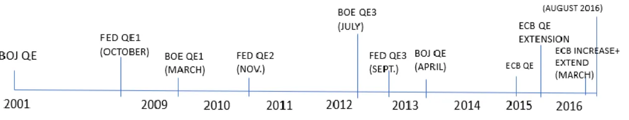
The US Federal Reserve started the quantitative easing in late November 2008 and the Bank of England in early 2009. Even if the Bank of Japan resumed QE in 2012, they made earlier interventions such as the one in March of 2001.
Diagram 1: Timeline of Central Bank’s Unconventional Monetary Policy decisions
Source: Author’s own elaboration.
Although the operational framework has not changed in a fundamental way, the ECB continues to lend whereas the FED, BoE and other Central Banks continue to buy and sell securities in their open market operations. This reflects, respectively, the bank-based financial system of the Euro Area and the capital market-based financial system of the US. In addition, the effectiveness of ECB measures in comparison with those of the FED and BoE is also related to the absence of banking and fiscal union, market fragmentation and heterogeneities within the Eurozone (Pisani-Ferry and Wolff, 2012).
22 The Bank of England Asset Purchase Facility was announced on 19 January 2009, as it can be seen in the graph below. However, the BoE announced in March 2009 a new policy of asset purchases to break with the past policies, and reduced bank rate to 0,5%. In total, from March 2009 to January 2010, £200 billion of assets were purchased. The bank rate is the interest that commercial banks received for holding Central Bank money as reserves. These injections facilitated UK banks to finance higher levels of liquid asset and to extend new loans. Consequently, household’s consumption and investment are supported and the Central Bank succeed when influencing asset prices through the bank lending channel.
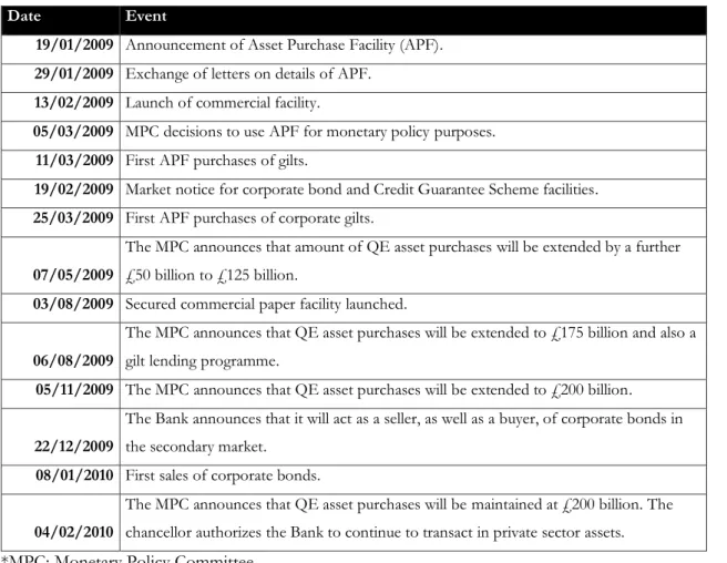
Table 2: First round of bond purchases under the QE program by the Bank of England.
Date Event
19/01/2009 Announcement of Asset Purchase Facility (APF). 29/01/2009 Exchange of letters on details of APF.
13/02/2009 Launch of commercial facility.
05/03/2009 MPC decisions to use APF for monetary policy purposes. 11/03/2009 First APF purchases of gilts.
19/02/2009 Market notice for corporate bond and Credit Guarantee Scheme facilities. 25/03/2009 First APF purchases of corporate gilts.
07/05/2009
The MPC announces that amount of QE asset purchases will be extended by a further £50 billion to £125 billion.
03/08/2009 Secured commercial paper facility launched. 06/08/2009
The MPC announces that QE asset purchases will be extended to £175 billion and also a gilt lending programme.
05/11/2009 The MPC announces that QE asset purchases will be extended to £200 billion. 22/12/2009
The Bank announces that it will act as a seller, as well as a buyer, of corporate bonds in the secondary market.
08/01/2010 First sales of corporate bonds. 04/02/2010
The MPC announces that QE asset purchases will be maintained at £200 billion. The chancellor authorizes the Bank to continue to transact in private sector assets.
*MPC: Monetary Policy Committee
Source: Own elaboration based on the information retrieved from the Bank of England.
Empirically, Lyonnet and Werner (2012) proved that BOE’s QE of 2009 did not have the desired results, since total assets were not positively correlated with nominal GDP and interest rates were not negatively correlated. On the contrary, the study conducted by Kapetanios et. al (2012) estimating three different time-series models showed that QE was crucial for real GDP and inflation not to fall. Nonetheless, the econometrics applied on QE
23 studies are subject, on the one hand, to endogeneity problems due to the change in macroeconomic variables, and on the other hand, to short period-time analysis, which complicates the application of estimators, and thus, influences the results.
Between September 2016 and April 2017, BoE purchased corporate bonds up to £10 billion through auctions, with the aim of stimulating both bond issuance and portfolio rebalancing (Bank of England, 2016). The economic literature focused on an unintended impact on liquidity, in fact, I stated that it improved the liquidity of corporate bond market (Boneva et al., (2019).
Belke et al. (2017) estimated the relationship between US and euro-area interest rates and found little evidence between the relationship of the FED’s asset purchases and the trans-Atlantic interest rate. In this case it is possible to talk about a “perfect interest rate spill-over” even if it is not compatible with the portfolio rebalance approach. The biggest institutional investors are usually required to invest in their home currency; thus, it is difficult to rationalize from a portfolio-balance point of view that bond-buying by the FED should have exactly the same impact on safe euro area long-term interest rates as in the US.
To measure the effects of the Unconventional Monetary Policy on asset prices most authors use event-study methodologies but Rogers et al., (2014), made an emphasis on inter-daily data since most monetary policy announcements have been coming out gradually prior to the announcement. They found out that cross-country spillovers are greater from the US to non-US yields than the other way around, and also that the UMP effects are larger in stock prices rather than in government bonds.
Table 3 displays the actions taken by the FED in order to show an overlook regarding the three issuance of asset purchases that they have conducted until the moment of writing this article.
24
Table 3: Decisions taken by the FED regarding QE programme.
Date Events
25/11/2008 Announce plan to purchase $100B in direct debt and $500B in MBS*
16/12/2008 Evaluation of the benefits of purchasing longer Treasury bonds.
18/03/2009 Expansion of MBS to $1,25 trillion & buy $300 billion in longer-term Treasury bonds.
31/05/2010 QE1 closure because of its completion at the end of the first quarter of 2010
27/08/2010 Ben Bernanke gives hints about QE2
03/11/2010 QE2 Announcement: To buy $600 billion in bonds
30/06/2011 QE2 closure because of its completion at the end of the second quarter of 2011
21/09/2011
Movement to lower interest rates on consumer loans with a $400 billion debt-swap program
31/08/2012 Ben Bernanke gives hints about QE3
13/09/2012 QE3: buy $40 billion of agency MBS* per month.
29/10/2014 QE3 closure
14/06/2017
In October, the Committee will initiate the balance sheet normalization program described in the June 2017 Addendum to the Committee’s Policy Normalization Principles and Plans.
*MBS: Mortgage-Backed Securities
Source: Own elaboration based on the information retrieved from the Federal Reserve
According to Krugman (1998), the inefficiency of monetary easing arises when interest rates are close to be zero and blame Japan of falling into a liquidity trap. In fact, the Japanese QE policy applied endured five years, from March 2001 to March 2006. They started the QE with a target of five trillion yen but in 2001, the required reserve level was four trillion yen. As the economy worsened, the target increased to 35 trillion yen in January of 2004. Japanese QE consisted on three actions: To provide ample liquidity to realize a current account balance target; To commit to the maintenance of the QE on the expected future path of short-term interest rates; and finally, to increase the purchases of long-term Japanese Government Bonds. The commitment was consistent with Krugman’s idea to raise inflation in an economy confronting a liquidity trap: to promise not to raise interest rates even if the economy has started to expand and prices have started to rise. He argued that with negative interest rates and declining prices, an expansionary policy is ineffective since nominal interest rate cannot be reduced below zero percent.
Empirical results show that Japanese QE had its biggest impact through the channel that works on the expected future path of short-term interest rates. Indeed, they committed to
25 maintain low the short-term interest rates until Consumer Price Index turned stable (Ugai H., 2007).
6. DATA AND EMPIRICAL APPROACH 6.1. Data
Bank balance sheet information is retrieved from Bureau van Dijk’s Bankscope, Orbis Bank Focus. The sample consists of quarterly based information for a sample of Eurozone banks covering the 2002Q1-2016Q4 period.6 I include consolidate balance sheets and income statements of commercial banks, savings banks, and credit unions. All the banks included in my sample displays financial information from the 1st January to 31st December. Lastly, I remove ambiguity and double counting of banks by selecting financial statements at the highest level of consolidation possible, usually as banking groups.
The data are expressed in thousands of euros and is inflation adjusted. For consistency purposes, I have eliminated values representing zero total assets, zero employees and negative balance sheet values. Finally, my data has resulted in a total of 11,460 number of observations constructed over 191 banks (individuals) and across 60 quarters.
The years that are covered by the sample are relevant because they reflect the pre-crisis period (2002Q1-2007Q2), the beginning of the banking and the European sovereign debt crisis (2007Q3-2016Q4), and the period in which the APP was implemented (2015Q1-2016Q4).
Finally, macroeconomic information was retrieved from the Thomson Reuters Datastream database.
Table A1 in the Annex section contains the definitions of the study variables employed in this paper.
6 The Eurozone Members included in our sample are Austria, Belgium, Cyprus, Estonia, Finland, France, Germany, Greece, Ireland, Italy, Latvia, Lithuania, Luxembourg, Malta, Netherlands, Portugal, Slovakia, Slovenia, and Spain.
26
6.2. Empirical approach
This section discussed the identification strategy to estimate the effects of the ECB’s QE on credit supply, bank market concentration, and financial stability.
Our empirical strategy is based on the following OLS model with structural break as follows: 𝑦𝑖𝑡 = 𝛽0+ 𝛽1𝑄𝐸𝑡+ 𝛽2𝑀𝑃𝑡+ 𝛽3𝑄𝐸𝑡× 𝑀𝑃𝑡+𝑋𝑖𝑡−1′ Φ + ϵi+ εt+ 𝜐𝑖𝑡 (1)
Dependent variables (yit): First, we use the ratio credit to customers over bank’s total assets
(LOANTAit), which measures credit supply. Second, we include the Herfindhal-Hirshman Index (HHIt)7 for loans and deposits which measures bank market concentration for lending and deposit markets, respectively. The HHI is computed as the squared sum of market share for loans (HHI_LOANit) and deposits (HHI_DEPOit). Lastly, we compute the logarithm of the Z-score (ln(Zit)) to measure financial stability8. This indicator has been extensively used in the financial stability literature (Laeven and Levine, 2009; Schaeck et al., 2012; Liu et al., 2013; Köhler, 2015). By using accounting information on bank profitability, volatility, and capitalization, the Z-score is defined as follows:
𝑍𝑖𝑡 =𝑅𝑂𝐴𝑖𝑡+ 𝐶𝐴𝑅𝑖𝑡
𝜎(𝑅𝑂𝐴𝑖𝑡) (2)
where ROAit represents the return on assets which is computed as profit (or losses) before taxes over total assets, CARit is the capital over total assets, and σ(ROAit) represents the standard deviation of total assets. We used a three-year rolling window for σ(ROAit) to allow time variability in the denominator and prevent Z to exclusively depend on the variation of profitability and capital cushion.
The Z-score measures the inverse probability of bank’s default.
Explanatory variables (X’it): Indicators of monetary policy are captured by the variable
MPt, which is the target variable, and includes EURIBORt , EONIAt and monthly net purchases (Monthlynetpurcht) for each quarter t. Matrix X’it is a set of control variables which includes the following one-period lagged variables: the income structure variable (INCi,t-1), computed as non-interest income over total assets controlling business diversification; bank’s
7 For further information about the index, see: Albert O. Hirschman, "The Paternity of an Index," American Economic Review (September 1964), pp. 761-62.
8 For more information regarding Financial Stability, see the “Financial Stability Review” published by the ECB every two years in its website.
27 size (Sizei,t-1), computed as the natural logarithm of one-period lagged total assets; return on assets (ROAi,t-1) and capitalization (CARi,t-1) representing profitability and bank’s equity, respectively; and, bank’s efficiency (EFFi,t-1), computed as operating cost over gross income.
We include the following macroeconomic controls at the country level (h):, the unemployment rate (UNh,t-1), the harmonised inflation rate (HICPh,t-1) and GDP growth (GDP h,t-1). A difference-in-difference variable is included (MPt × QEt) to estimate the impact of the negative interest rates as a consequence of the crisis in the dependent variables. This approach is used to test the treatment effect apply by the ECB and compare the situation before and after QE. Besides, the analysis of the impact in EURIBOR (in 1, 3, 6 and 12 months) and EONIA exert the macroeconomic effects of the policy. Finally, the variables єi and εt are included to control for the individual and time effects, respectively.
6.3. Hypotheses
The aim of this research is to analyze the effect of QE and the crisis on credit supply, market concentration and financial stability. Based on the background information, the following hypotheses are tested:
Hypothesis 1: Lending supply increases after the QE programme.
Hypothesis 2: Lending and deposits market increase concentration after the QE programme. Hypothesis 3: Financial stability increases after the QE programme.
7. EMPIRICAL RESULTS
Table 4 reflects the summary statistics for all the variables used in the regressions. The credit supply (LOANTAit), has a mean value of 0.59 percent and ranges between 0.04 and 0.92 percent. The statistical measure of concentration for loans and deposits (HHI_LOANit and HHI_DEPOit) displays a mean value around 0.37 for both markets, ranging from 0 to 1. The financial stability, represented by the logarithm of the Z-score (Ln(Zit)), shows a mean value of 1.69 ranging from -5.89 to 4.96. Besides, the macroeconomic interest rates (EONIAt, Monthlynetpurcht, EURIBOR1t, EURIBOR3t, EURIBOR6t, and EURIBOR12t), show a positive mean value sign, which indicates that over the analyze period they have followed a positive trend. Finally, the dummy variables (Crisist and QEt), display a mean value of 0.63 and 0.13 respectively, meaning that the 63% of our sample are included in crisis period and the 13% in QE period.
28
Table 4: Descriptive Statistics
This table displays the distribution of the variables used in this study over the period of 2002Q1 to 2016Q4.
N Mean St.Dev. Min. Pc. 25 Median Pc.75 Max.
Dependent variables LOANTAit 11,460 0.58888 0.2127 0.0410 0.4583 0.6315 0.7576 0.9285 HHI_LOANit 11,460 0.37115 0.3188 0.0000 0.0000 0.3580 0.5317 1.0000 HHI_DEPOit 11,460 0.37895 0.3222 0.0000 0.0000 0.35350 0.5220 1.0000 ln(Zit) 11,460 1.6915 0.9213 -5.8953 1.1363 1.6624 2.2430 4.9625 Explanatory variables INCit 11,460 0.37468 0.2822 -0.1152 0.2075 0.30986 0.4459 1.4796 Monthlynetpurch 11,460 7672.9 2693.5 3266.3 6089.67 7600.0 9895.33 11388 EONIAt 11,460 1.4882 1.4554 -0.3485 0.1230 1.0087 2.7337 4.2527 EURIBOR1t 11,460 1.5995 1.5058 -0.3715 0.1566 1.3121 2.7442 4.5394 EURIBOR3t 11,460 1.7394 1.5281 -0.3124 0.2537 1.5284 2.8430 4.9817 EURIBOR6t 11,460 1.8579 1.4995 -0.2133 0.3741 1.7431 2.9673 5.1756 EURIBOR12t 11,460 2.0252 1.4769 -0.0744 0.5697 2.1209 2.9969 5.3678 Sizeht 11,460 23.296 2.1284 17.399 21.886 23.026 24.6151 28.273 ROAit 11,460 0.0040839 0.0161 -0.0923 0.0017 0.0057 0.0107 0.0378 CARit 11,460 0.081456 0.0408 0.0160 0.0550 0.0730 0.100 0.2516 EFFit 11,460 0. .32707 0.1779 0.0002 0.2285 0.2873 0.3729 1.2018 GDPt 11,460 0.015126 0.0323 -0.1930 0.0043 0.0156 0.0296 0.2760 HICPt 11,460 1.9705 1.8140 -3.8667 0.8666 1.9333 2.7000 17.533 UNit 11,460 9.0926 4.3690 2.1333 6.0000 8.4333 10.3333 26.200 Crisist 11,460 0.63333 0.4819 0.0000 0.0000 1.0000 1.0000 1.0000 QEt 11,460 0.13333 0.3399 0.0000 0.0000 0.0000 0.0000 1.0000
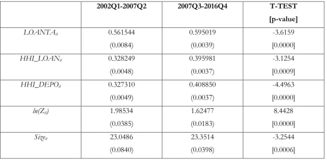
29 Table 5 shows a mean-difference test constructed after the creation of two dummy variables. On the one hand, crisist takes the value 1 from 2007Q3 to 2016Q4, and zero otherwise. On the other hand, QEt takes the value 1 from 2015Q1 to 2016Q4 and zero, otherwise. The results suggest the existence of a structural break in the key variables employed in this study as a consequence of the implementation of the QE.
Table 5: Parametric tests for the comparison of means for the pre-crisis (2002Q1-2007Q2), crisis period (2007Q3-2015Q1), and the QE period (2015Q2-2016Q4).
This table split the sample into two periods: before the crisis (2002Q1 – 2007Q2) and after the crisis (2007Q3 – 2016Q4). The parametric test is conducted under the null hypothesis H0: Crisis(0) – Crisis (1) = 0 for the precrisis the post-crisis periods. All the variables are defined in Table A.1. Panel A shows the results for the whole sample period of analysis. Panel B shows the results for the pre-crisis period and the period between the beginning of the crisis and the implementation of the QE. The coefficients are for the mean values, while the standard errors are goven in parenthesis. The p-value of the Student t-statistics is shown in the third column of each period of analysis.
Panel A: Ordinary Least- Square regression model to test and compare the means before the crisis (2002Q1 – 2007Q2) and after the crisis (2007Q3 – 2016Q4)
2002Q1-2007Q2 2007Q3-2016Q4 T-TEST [p-value] LOANTAit 0.561544 (0.0084) 0.595019 (0.0039) -3.6159 [0.0000] HHI_LOANit 0.328249 (0.0048) 0.395981 (0.0037) -3.1254 [0.0009] HHI_DEPOit 0.327310 (0.0049) 0.408850 (0.0037) -4.4963 [0.0000] ln(Zit) 1.98534 (0.0385) 1.62477 (0.0183) 8.4428 [0.0000] Sizeit 23.0486 (0.0840) 23.3514 (0.0398) -3.2544 [0.0006]
30
Panel B: Ordinary Least- Square regression model to test and compare the means before the QE (2007Q1 – 2015Q1) and after the QE (2015Q2 – 2016Q4).
2007Q3-2015Q1 2015Q1-2016Q4 F-TEST [p-value] LOANTAit 0.5978 (0.0045) 0.5817 (0.0098) 1.4551 [0.0729] HHI_LOANit 0.2982 (0.0031) 0.2582 (0.0059) 5.6305 [0.0000] HHI_DEPOit 0.3106 (0.0030) 0.2658 (0.0059) 6.4201 [0.0000] ln(Zit) 1.6419 (0.0197) 1.5290 (0.0346) 2.3084 [0.0105] Sizeht 23.3262 (0.0434) 23.4835 (0.0995) -1.4488 [0.0738]
The results I obtained in Panel A, reject the null hypothesis (H0: Crisist (0) – Crisist (1) = 0) at a 99% confidence level for every variable. Therefore, the alternative, which states that the mean value of the variables change with the crisis is confirmed. One of the implications of the results is that HHI increases during the crisis for deposits and loans, and thus, their concentration. The market is more concentrated due to the multiple banking fusions that took place with the financial break (ECB, 2016). The implications of the fusions are in line with the obtained results since bank’s size increase even though it does not show a big difference. The results also suggest that LOANTAit increases, meaning that with the crisis there is more accumulated credit in the market, or in other words, there are outstanding volumes in the balance sheet of the banks. The implications of the fusions are in line with the obtained results since bank’s size increase. It is, therefore, possible to state that the banks with the biggest dimensions, due to the fusions or to the crisis itself, are the ones that more credit accumulate. Finally, the numbers show that the mean value for financial stability (ln(Zit)) decrease after the break. The results are consistent with the situation of the Euro Area, indeed, with the aim of preserving stability, the ECB addressed more ambitious macroprudential policies (see De Guindos, 2018).
In Panel B, we show that the parametric test does not reject the null (H0 : QEt(0) − QEt(1) = 0) for the variables LOANTAit, HHI_LOANit and ln(Zit). Conversely, the null is rejected, and thus, the alternative (H0: QEt(0) − QEt(1) > 0 ) is confirmed for Sizeht and HHI_DEPOit
31 the credit and deposit markets act as two independent markets. Importantly, the fact that the null confirms for LOANTAit, indicates that QE has not been effective with respect to credit
supply, even though the objective of the ECB was to activate the market. In regards to the financial stability (ln(Zit)), the null is confirmed and the mean test shows a decrease in the period of QE. The economic literature has been actively focused on the role that the ECB plays achieving financial stability, when in reality and as shown previously in panel A, financial stability is a focus in macroprudential policies more than in QE itself. My results are in accordance with this statement since the QE has not been able to reach to the desire financial stability levels.
Bank’s dimension (Sizeht) is statistically significant and slightly positive in both panels, since some banks in the sample were merged or integrated with other banks, after restructuring processes or endevours to create national champions.
7.1 The baseline regression
This section analyzes the impact that the financial crisis and the QE had on credit supply, market concentration and financial stability, using the variables described in Table 4 with the descriptive analysis. The hypotheses are tested by means of a panel data regression with fixed effects. In the regression, in order to avoid endogeneity problems between the regressors and the dependent variables, I used one-period lagged explanatory variables.
The regression for monthly net purchases includes 307 number of observations since the programme began in March 2015.
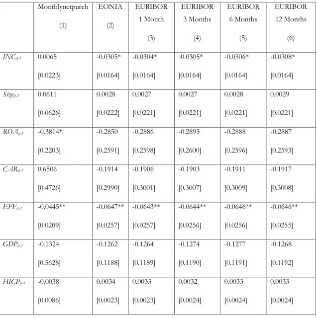
7.1.1 The effects of QE on credit supply
The first research question discusses in what extent had monetary policy changed bank’s credit supply. The empirical results, reported in Table 6, show significance in the efficiency ratio for every column, meaning that as the more efficient the bank is, the less credit will supply. Results also display that the effects of QE decrease credit supply when actually it is supposed to expand credit in order to boost economic growth. Nonetheless, due to the crisis, the repayment capacity of households and firms decrease, increasing their probability of default. Even though the liquidity injections from the ECB increase the ability of banks to supply credit, the most affected ones may prefer to use the reserves to deleverage and reduce the amount of non-performing loans on their balance-sheets. The need for deleverage is also
32 displayed in customers portfolio decreasing the demand for credit in the Euro Area, and offsetting the effects of the liquidity injections as a result of the QE.
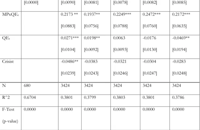
Table 6: The effects of the crisis and the unconventional monetary policy on lending supply from 2002Q1 to 2016Q4.
The table shows the results of the effects of the QE on lending supply. The dependent variable is LOANTAit.
To test for structural breaks, I include the dummy variable Crisist defined in “Panel A” , which takes the value 1 from 2007Q3 onwards (𝑡 ≥ 2007𝑄3), and zero otherwise. This table is organized in columns, where different macroeconomic interest rates are specified (MPt). Variable QEt takes the value one from 2015Q2 onwards, and zero otherwise. The MPtxQEt variable interaction represents the effect of the ECB’s QE. Column
(1) includes observations from 2007Q3 until 2016Q4. Columns (2)-(6) include observation from 2002Q1 to 2016Q4. The *. **, *** on the right of the coefficients state whether the estimations are statistically significant at the 10, 5 and 1% level, respectively.
Monthlynetpurch (1) EONIA (2) EURIBOR 1 Month (3) EURIBOR 3 Months (4) EURIBOR 6 Months (5) EURIBOR 12 Months (6) INCit-1 0.0065 [0.0223] -0.0305* [0.0164] -0.0304* [0.0164] -0.0305* [0.0164] -0.0306* [0.0164] -0.0308* [0.0164] Sizeit-1 0.0611 [0.0626] 0.0028 [0.0222] 0.0027 [0.0221] 0.0027 [0.0221] 0.0028 [0.0221] 0.0029 [0.0221] ROAit-1 -0.3814* [0.2203] -0.2850 [0.2591] -0.2886 [0.2598] -0.2895 [0.2600] -0.2888 [0.2596] -0.2887 [0.2593] CARit-1 0.6506 [0.4726] -0.1914 [0.2990] -0.1906 [0.3001] -0.1903 [0.3007] -0.1911 [0.3009] -0.1917 [0.3008] EFFit-1 -0.0445** [0.0209] -0.0647** [0.0257] -0.0643** [0.0257] -0.0644** [0.0256] -0.0646** [0.0256] -0.0646** [0.0255] GDPit-1 -0.1324 [0.5628] -0.1262 [0.1188] -0.1264 [0.1189] -0.1274 [0.1190] -0.1277 [0.1191] -0.1268 [0.1192] HICPit-1 -0.0038 [0.0086] 0.0034 [0.0023] 0.0033 [0.0023] 0.0032 [0.0024] 0.0033 [0.0024] 0.0033 [0.0024]