Working Paper/Document de travail
2008-9
A Model of Housing Boom and Bust
in a Small Open Economy
Bank of Canada Working Paper 2008-9
April 2008
A Model of Housing Boom and Bust
in a Small Open Economy
by
Hajime Tomura
Monetary and Financial Analysis Department
Bank of Canada
Ottawa, Ontario, Canada K1A 0G9
htomura@bankofcanada.ca
Bank of Canada working papers are theoretical or empirical works-in-progress on subjects in economics and finance. The views expressed in this paper are those of the author.
Acknowledgements
I thank Jason Allen, Thomas Carter, Jonathan Chiu, Ian Christensen, Ali Dib, Walter Engert,
Césaire Meh, Miguel Molico, Fuchun Li, Shin-ichi Nishiyama, Yaz Terajima and
Alexander Ueberfeldt for their comments. Thomas Carter provided superb research assistance.
All the errors are my own.
Abstract
This paper considers a dynamic stochastic general equilibrium model for a small open economy
and finds that an improvement in the terms of trade causes a housing boom-bust cycle if the
duration of the improvement is uncertain. It is shown that as the economy has better access to the
international financial market, the extent of the housing boom and bust gets larger. Also, an
increase in the loan-to-value ratio in the domestic mortgage market tends to enhance the extent of
the housing boom and bust when the economy has good access to the international financial
market.
JEL classification: E44, F41
Bank classification: Business fluctuations and cycles; Credit and credit aggregates
Résumé
À l’aide d’un modèle d’équilibre général dynamique et stochastique qui décrit une petite
économie ouverte, l’auteur montre qu’une amélioration des termes de l’échange provoque une
flambée des prix du logement puis leur effondrement si la durée de cette amélioration est
incertaine. Il constate qu’un meilleur accès de l’économie au marché financier international a pour
effet d’accentuer l’ampleur du cycle des prix observé et que, lorsque l’économie a facilement
accès à ce marché, une augmentation du ratio prêt-valeur sur le marché hypothécaire national tend
à amplifier encore le cycle.
Classification JEL : E44, F41
1
Introduction
This paper presents a model of housing boom and bust in a small open economy that emphasizes the role of the terms of trade (the price of exports relative to that of imports)1 in determining house prices. This analysis is motivated by recent experience in Canada, where since the late 1990s mounting house prices have been accompanied by a significant improvement in the terms of trade and a significant rise in the real value of Canadian GDP measured using the real effective exchange rate or the command GDP.2 This observation suggests that as the terms of trade improve, the trading value of Canadian output increases and households enjoy an increase in the real value of their income in terms of purchasing power over imported goods. Higher household income then contributes to a strengthening in housing demand and rising house prices. Here changes in the terms of trade are regarded as exogenous shocks, as Canada is a small open economy and the prices of Canadian exports and imports are largely determined in world markets. Considering the terms of trade as important exogenous shocks to a small open economy is consistent with the international business cycle literature, which finds that terms-of-trade shocks are quantitatively important sources of business cycles in small open economies.3 Also Kohli (2004) finds that change in the terms of trade accounts for a significant fraction of the real income growth in a sample of 26 OECD countries for 1980-1996.
The model in this paper captures the effect of the terms of trade on house prices and shows that if households are uncertain about the duration of an improvement in the terms of trade, then house prices will abruptly drop when the terms of trade stop improving. Expectations of households play a key role in causing the housing boom-bust cycle. So long as the terms of trade are improving, households expect that the real value of domestically produced goods will continue to rise. As
1
The usual definition of the terms of trade in the literature is the price of imports relative to that of exports. I invert the usual definition as it is convenient for presentation in this paper.
2
The command GDP estimates real output taking into account terms-of-trade changes by deflating current-dollar exports by an import price index. See Kohli (2004) for more detail on the concept of the command GDP.
3
For example, Easterly, Kremer, Pritchett and Summers (1993) study a large panel of countries and find that terms-of-trade shocks have significant effects on the GDP growth rates. Mendoza (1991, 1995) and Kose (2002) calibrate dynamic stochastic general equilibrium models, and find that terms-of-trade shocks are quantitatively important sources of business cycles in small open economies. Note that Mendoza (1991) calibrates the model to the Canadian economy. Also Macklem (1993) analyzes the effects of long-run and short-run changes in the terms of trade using dynamic general equilibrium multi-sector models calibrated to the Canadian data. Macklem considers a over-lapping generation model with stochastic death and investigates the effect of the terms of trade on sectoral production as well as aggregate production. Backus and Crucini (2000) find a role for fluctuations in oil prices in international business cycles including effects on the U.S. economy through changing the terms of trade across countries.
this will increase future purchasing power, households expect stronger housing demand and higher house prices in the future. This leads to an increase in current house prices. But when the terms of trade stop improving, households correct their expectations regarding future house prices, and current house prices abruptly drop.
This mechanism is similar to the findings of Zeira (1999) and Barbarino and Jovanovic (2007), each of whom considers a boom-bust cycle in stock prices when firms experience an expansion in market size for their products but the duration of the expansion is uncertain. While their work considers partial equilibrium models taking the interest rate as exogenous, in this paper I endogenize the determination of the domestic interest rate in a small open economy. I find that the domestic interest rate rises when the terms of trade are improving, since the increase in the expected purchasing power of future income subdues the need to save so as to ensure consumption-smoothing. As current house prices are partly determined by the present discounted value of expected future house prices, the rise in the domestic interest rate partially offsets the size of the increase in house prices during the boom by increasing the discount rate applied to expected future house prices. When the terms of trade stop improving, the expected purchasing power of future household income declines, which reduces the domestic interest rate. The decline in the domestic interest rate in turn mitigates the abrupt drop in house prices after the boom.
This role of the domestic interest rate in determining the extent of the housing boom-bust cycle implies that as the economy has better access to the international financial market, the extent of the housing boom and bust becomes larger. This is because the international financial market absorbs a greater portion of changes in domestic credit supply and demand, so that fluctuations in the domestic interest rate are attenuated.
I also consider how the extent of housing boom and bust depends on the loan-to-value ratio in the domestic mortgage market. I find that an increase in the loan-to-value ratio has two opposite effects. The first effect is the financial accelerator effect analyzed by Bernanke and Gertler (1983), Kiyotaki and Moore (1997) and Iacoviello (2005), which enhances the extent of the housing boom and bust. In this narrative, a higher loan-to-value ratio bolsters the boom since more credit is available to finance investments in housing. However, the bust is exacerbated since more housing collateral must be liquidated to service larger debts. The second effect is the domestic interest rate effect. The higher loan-to-value ratio renders household borrowing capacity more sensitive
to changes in house prices and encourages wider fluctuations in the domestic interest rate, which dampens the housing boom-bust cycle. I find that the first effect tends to dominate the second when the economy has good access to the international financial market, which makes fluctuations in the domestic interest rate small.
I calibrate the model to the Canadian economy and show that the mechanism presented in this paper can contribute to causing housing booms and busts of non-trivial magnitude if households expect a persistent improvement in the terms of trade, although it cannot account for the full extent of the cycles observed in the data. Hence, the mechanism analyzed in this paper is complementary to the other possible contributors to housing boom-bust cycles.
The rest of the paper is organized as follows. Section 2 briefly summarizes the recent observation in Canada. Section 3 describes the model. Section 4 shows the dynamics of the model when the terms of trade improve but the duration of the improvement is uncertain. Section 5 investigates the effect of financial market efficiency. Section 6 concludes.
2
Recent experience
2.1 Terms of trade and house prices in Canada
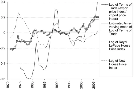
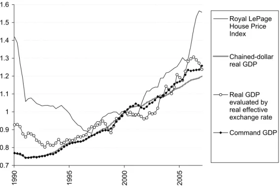
Figure 1 shows that Canadian house prices have been increasing since the late 1990s and that the housing boom has coincided with an improvement in the terms of trade. Figure 2 illustrates that the improvement in the terms of trade has increased the trading value of Canadian output, and that the real value of Canadian GDP in terms of purchasing power over imported goods has been growing faster than the standard chained-dollar real GDP. Figure 2 shows two measures of the real value of Canadian GDP in terms of purchasing power over imported goods: the value of Canadian GDP evaluated using the real effective exchange rate and the command GDP. The command GDP is the sum of the real value of consumption, investment and government expenditures plus the nominal value of net exports deflated by an import price index. This measure takes terms-of-trade changes into account when measuring real GDP. As the chained-dollar real GDP measures the quantity of output, the difference in the speed of growth between the chained-dollar real GDP and the two alternative measures reflects an increase in the trading value of Canadian output.
in the terms of trade may have contributed to strengthening in housing demand and rising house prices. Here I highlight a role of the terms of trade in effecting fluctuations in house prices, since the international business cycle literature identifies the terms of trade as one of the driving forces behind business cycles in small open economies. The changes in the terms of trade are regarded as exogenous shocks to a small open economy, since export and import prices for small open economies are largely determined in world markets.
The pattern of house prices across provinces also suggests that the terms of trade affect house prices. Figure 3 shows the prices of export and import goods deflated by the GDP deflator.4 Each price series in the figure is weighted by the average share of the total nominal value of merchandise exports or imports for which the tradable goods in question account over the period 1997-2007. Hence the change in each series reflects the size of its impact on the overall terms of trade. The figure illustrates that the recent improvement in the terms of trade is driven by a rise in the energy prices such as oil, gas and coal since 1999 and reinforced by a decline in the prices of manufactured goods since 2002. As energy and manufactured goods are respectively important export and import goods for Canada, these price movements together improve the terms of trade. These trends coincide with the pattern of provincial house prices in Canada described in Table 1: western Canada has experienced stronger growth in house prices than have the eastern provinces, and has a higher share of oil, gas and mining and a lower share of manufacturing in total value-added production. This observation could be interpreted as suggesting that shocks to the terms of trade affected local purchasing power differentially on account of differences in industrial production profiles between provinces.5
2.2 Terms of trade and house prices in developed small-open economies
Table 2 compares changes in the command GDP, the real GDP, the terms of trade and the real house price for 1999-2006 among a sample of developed small-open economies.6 I choose the 1999-2006
4
The sample period is limited as the current series of the price indexes for merchandise trade only dates back to 1997.
5
I will consider fluctuations in aggregate house prices abstracting from provincial heterogeneity. The first column in Table 1, which includes the prices of existing houses, shows house prices have been strongly growing across Canada in the recent period. The analysis in this paper is complementary to the role of local determinants of house prices. Allen, Amano, Byrne and Gregory (2006) find local factors play an important role in determining house prices in each major Canadian city.
6
Table 1: Provincial house prices and industrial production profiles
Cumulated growth of Cumulated growth of Share of Oil, Share of Royal LePage House New House Price Gas and Mining Manufacturing Price Index for ’99-’06 Index for ’99-’07 in the province in the province
St. John’s - 7.7% 17.9% 7.3% Halifax 29.6% 3.1% 3.6% 12.2% Montreal 31.6% 20.8% 0.7% 23.5% Ottawa 48.0% 28.1% 0.8% 24.0% Toronto 32.9% 7.3% 0.8% 24.0% Winnipeg 48.7% 19.4% 2.1% 14.4% Regina - 23.1% 17.7% 7.8% Saskatoon - 16.9% 17.7% 7.8% Edmonton 58.2% 60.5% 24.4% 10.1% Calgary 83.8% 73.8% 24.4% 10.1% Vancouver 46.1% 1.6% 3.8% 12.5%
Notes: The first and second columns are respectively the total growth rates of the Royal LePage House Price Index for 1999:1Q-2006:2Q and the New House Price Index for 1999:1Q-2007:1Q. The Royal LePage House Price Index includes the prices of existing houses, while the New House Price Index only covers the prices of new houses. Both indices are deflated by the GDP deflator. Estimates of the Royal LePage House Price Indices at the city level are provided by the Centre for Urban Economics and Real Estate of the University of British Columbia, http://cuer.sauder.ubc.ca/cma/index.html. ’−’ indicates that the centre does not provide the estimate for the city in question. The third and forth columns are respectively the average shares of Extraction of Oil and Gas and Mining and Manufacturing in total value-added production in the province where each city is located. The sample period of these shares is for 1997-2003 due to data availability. The cities are ordered from east to west.
period as the sample period in order to summarize the change in the terms of trade and real domestic income during the recent housing booms in many countries. The table indicates that the correlation coefficient between the command GDP growth and the real house price growth is 0.27. This significantly positive correlation supports the view that an increase in the real household income generates a housing boom, provided that the command GDP is a good measure of real income for a country.7 The third column of the table then shows how much fraction of the command GDP growth is unaccounted for by the real GDP growth for each country. Note that discrepancy between the command GDP growth and the real GDP growth is caused by terms-of-trade change. The third and forth columns indicate that terms-of-trade changes significantly contributed to increases in real income for resource-exporting countries in the sample, that is, Australia, Canada and Norway, in the 2000s.
2.3 Structural change in the Canadian terms of trade
2.3.1 Structural break test
Figure 1 indicates that the recent improvement in the Canadian terms of trade is a departure from the stable mean that had prevailed for the 1980s and the 1990s. This is confirmed by the Bai-Perron (1998) structural break test. I consider the following regression for the terms of trade:
ln(Zt) =µZ,j+eZ,t, fort = τZ,j−1+ 1, τZ,j−1+ 2, ... , τZ,j and j = 1, ... , mZ+ 1, (1)
whereZtis the terms of trade defined as the export price index divided by the import price index,8
t is the time, µZ,j is the mean of the terms of trade in the j-th regime which ends in the date
τZ,j, and eZ,t is the error term. τZ,0+ 1 andτZ,mZ+1, respectively, are the initial date and the last
7
For the 1999-2006 period, the cumulated growth of the real GDP has a higher correlation coefficient with the cumulated growth of real house price, 0.52, than the cumulated growth of the command GDP. This observation reinforces the view that an increase in the real household income generates a housing boom, but also raises concern about the accuracy of the command GDP as a measure of real income. I still use the command GDP here in order to capture the effect of terms-of-trade change on real income, since it is a simple convenient measure. Also the command GDP becomes much more correlated with the cumulated growth of real house price for a longer sample period: The value of the correlation coefficient for the cumulated growth of the command GDP is 0.497 for 1980-2006, while that value for the cumulated growth of the real GDP is 0.486. This observation supports the use of the command GDP as a measure of real income. Note that the correlation coefficient takes the similar values not because the cumulated command GDP growth becomes identical to the cumulated real GDP growth in the long run. Consistent with the finding of Kohli (2004), I find that each country shows a significant discrepancy between the cumulated growth of the command GDP and the cumulated growth of the real GDP for the 1980-2006 period due to long-term changes in the terms of trade.
8
Table 2: Cumulated growth of key variables in developed small-open economies for 1999-2006
Command GDP Real GDP [(a)−(b)] Terms of trade Real house growth (a) growth (b) /[(a)−1] change price growth
Australia 1.362 1.248 0.313 1.428 1.524 Austria 1.134 1.145 -0.082 0.988 1.014 Belgium 1.121 1.146 -0.210 0.975 1.665 Canada 1.303 1.230 0.238 1.158 1.330 Denmark 1.190 1.139 0.264 1.068 1.574 Finland 1.177 1.248 -0.396 0.897 1.401 Greece 1.357 1.340 0.048 1.057 1.529 Ireland 1.456 1.483 -0.058 0.987 1.747 Netherlands 1.068 1.031 0.532 1.017 1.386 New Zealand 1.279 1.232 0.168 1.111 1.634 Norway 1.479 1.172 0.640 1.583 1.205 South Africa 1.330 1.303 0.080 1.065 2.213 Spain 1.290 1.277 0.042 1.024 1.820 Sweden 1.151 1.218 -0.439 0.918 1.644 Switzerland 1.116 1.122 -0.052 0.974 1.118
Notes: See appendix for the data sources. Figures in the columns 1-2 and 4-5 are the cumulated rate of change over 1999-2006, that is,x(2006)/x(1999), where x(t) denotes the value of the variable in question in yeart. The third column is the fraction of the command GDP growth that is not accounted by the real GDP growth. This figure indicates the contribution of terms-of-trade change to real income growth.
Table 3: Bai and Perron (1998) sequential test for the number of break points in the log of the terms of trade U Da max W Dmaxa F(2|1)b F(3 |2)b F(4|3)b F(5|4)b 1216.55∗∗ 2447.51∗∗ 65.94∗∗ 73.01∗∗ 73.01∗∗ 10.56 Notes: ∗ and ∗∗ mark 5% and 1% significance respectively. a One-sided
(upper-tail) test of the null hypothesis of 0 breaks against the alternative hypothesis of an unknown number of breaks given an upper bound of 5. b One-sided (upper-tail) test
of the null hypothesis ofℓbreaks against the alternative hypothesis ofℓ+ 1 breaks. In construction of the test, I use the global minimizers of the sum of the squared residuals of the regression.
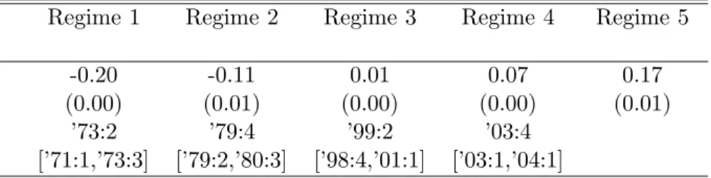
Table 4: Bai and Perron (1998) estimates of the mean and the end date of each regime for the log of the terms of trade
Regime 1 Regime 2 Regime 3 Regime 4 Regime 5
-0.20 -0.11 0.01 0.07 0.17
(0.00) (0.01) (0.00) (0.00) (0.01)
’73:2 ’79:4 ’99:2 ’03:4
[’71:1,’73:3] [’79:2,’80:3] [’98:4,’01:1] [’03:1,’04:1]
Notes: The first number in each cell is the estimated mean; standard errors are reported in parentheses. The end date is below the mean; 95% confidence intervals are reported in brackets.
date in the sample period. mZ is the number of structural breaks decided by the sequential test
recommended by Bai and Perron (2003). The set of coefficients {τZ,j, µZ,j}mj=1Z is jointly estimated by the method developed by Bai and Perron (1998).9
Table 3 reports the results of the sequential test on the number of break points. The test implies that there have been four breaks in the terms of trade at 1% significance level. Table 4 shows the estimates of the time-varying mean (µZ,j) and the end date (τZ,j) of each regime. Figure 1 plots
the estimated time-varying mean of the natural log of the terms of trade. The test result confirms that the Canadian terms of trade had a stable mean for the 1980s and the 1990s, but that there was a structural break in the end of the 1990s. In the 2000s, the terms of trade have been improving,
9
For the estimation, I use the GAUSS code accompanying Bai and Perron (2003) available from http://people.bu.edu/perron/code.html. For all the Bai and Perron estimation in this paper, I set 0.05 as the ratio of the minimum length of each regime to the sample length. Standard errors are heteroskedasticity- and autocorrelation-consistent (robust=1, prewhit=0, hetdat=1 and hetomega=1 in the options of the code).
departing from the stable mean before the 2000s.
As shown in Figure 3, the structural break in the end of the 1990s was caused by a persistent change in the world relative price between commodities and manufactured goods. This observation is consistent with Table 2 that shows that energy-exporting countries such as Australia, Canada and Norway have been experiencing significant improvements in the terms of trade in the 2000s. The improvements in the terms of trade may reflect a structural change in the world goods market such as heavily populated countries like China and India are increasing the supply of manufactured goods produced by their labour demanding more commodities for consumption and intermediate inputs.
2.4 Implication of the observations
Motivated by these observations, I suppose the current improvement in the Canadian terms of trade reflects a permanent mean shift and analyze its implication for the housing market constructing a dynamic stochastic general equilibrium model of a small open economy. I assume that the terms of trade will not keep improving forever, but will reach a new stable mean level, since it is impossible that the terms of trade increases to infinity. Also if the world economy reaches a balanced growth path, then the world relative prices of goods will be constant. In the following analysis, I consider how house prices fluctuate when it is uncertain how long an improvement in the terms of trade will last. In asking this question, I am motivated by the fact that households cannot be certain when the current improvement in the Canadian terms of trade, which began in the late 1990s, might end. This question is also motivated by historical considerations. Figure 1 shows that there were other significant improvements in the terms of trade in the early 1970s and around 1980 in Canada, which coincide with the structural break dates estimated by the Bai-Perron test. Also, these two periods are coincident with rapid rises in oil prices and housing boom-bust cycles, the former of which is also one of the features of the housing boom in the 2000s.10 The result of the model in this paper suggests that if households did not precisely know the durations of the improvements in the terms of trade, then this uncertainty could be one of the contributors to the housing boom-bust cycles.
10
The oil price significantly dropped in the mid-1980s. But this was not followed by a mean-shift in the Canadian terms of trade since a decline in the prices of manufactured goods offset the effect of the decline in the oil price on the terms of trade.
3
Model
3.1 Production functions
I construct a dynamic stochastic general equilibrium model for a small open economy based on Lubik and Teo (2005) and Iacoviello (2005). There is a continuum of households, which consume and invest final goods. Final goods are produced from two types of intermediate goods, home and foreign goods, according to the following function:
xt= xH,t 1−γ (1−γ) xF,t γ γ , (2)
wherextis the amount of final goods,xH,tis home goods andxF,tis foreign goods. The subscriptt
denotes the time period. Foreign goods must be imported from abroad. Home goods are produced by the standard Cobb-Douglas function
yt= (kt−1)α(Atnt)(1 −α)
, (3)
where yt is the amount of home goods produced, kt−1 is capital stock installed in the previous
period, At is total factor productivity (TFP), nt is employed labour hours, and α ∈ (0,1) is a
constant share of capital in production.
There are three types of stock in the economy: capital stock, residential structure and housing land. Housing land is non-reproducible and fixed-supplied. Capital stock and residential structure are produced from final goods and evolve according to the following laws of motion:
kt = (1−δK)kt−1+νK iK,t kt−1 ρK kt−1 (4) st= (1−δS)st−1+νS iS,t st−1 ρS st−1, (5)
whereiK,t is the investment of final goods into capital stock, δK is the depreciation rate for capital
stock, st is the stock of residential structure, iS,t is the investment of final goods into residential
structure, and δS is the depreciation rate for residential structure. The last term in each equation
is the adjustment cost function for each type of stock, where νi>0 and ρi ∈(0,1) fori=K, S.
3.2 Households
I consider two types of households. One type has a higher time-discount rate than the other. Fol-lowing Iacoviello (2005), I call the former type as ”patient”, and the latter type as ”impatient”.
This assumption enables me to model credit transactions across households and to analyze how fluc-tuations in house prices depend on the efficiency of the domestic financial market. The population of patient households is 1, and the population of impatient households ise(e >0).
Each patient household maximizes the utility function
E0 ( ∞ X t=0 (β′ )t hln(c′ t−ψv ′ t(n ′ t)φ) +θSln(s′t) +θLln(l′t) i ) , (6) where β′
∈ (0,1) is the time-discount rate, c′
t is consumption,n ′ t is labour hours, s ′ t is residential structure, and l′
t is housing land. The prime symbol (′) denotes variables for patient households.
The last two terms in the utility function indicate that households gain utility from housing services jointly provided by residential structure and housing land.11 v′
t is defined as v′ t= (c ′ t)η(v ′ t−1) 1−η . (7)
Here ψ,φ,θS and θL are positive constants, and η∈[0,1] .
As described by Jaimovich and Rebelo (2006), this utility function nests the Cobb-Douglas function (η = 1) and the Greenwood, Hercowitz and Huffman (1988) utility function (η = 0). These two functional forms have different implications for the response of labour supply when households expect a rise in future income. Under the Cobb-Douglas function, the rise in future income increases current consumption and raises the utility cost of labour supply. Thus labour supply declines. With the Greenwood-Hercowitz-Huffman utility function, this effect does not exist and labour supply is more responsive to the wage. In the dynamic analysis of the model, I will set a small positive value forηto ensure that labour supply increases during a housing boom as usually observed in data. A positive value forη is needed since there would be no balanced growth path under η = 0, around which I will solve the dynamic equilibrium by linearization. Even if I setη= 1 adopting the Cobb-Douglas utility function, the result of the model does not significantly change, except that a consumption boom increases disutility of labour enough to reduce both labour supply and output during a housing boom.
11
Land is included in the components of housing services here, since it is realistic. Also, without land, unreported calibration leads to only tiny fluctuations in the price of residential structure in the model, since the marginal adjustment cost of residential structure does not vary much. As shown below, calibration with land implies a different set of parameter values with which house prices vary in response to shocks due to fixed-supplied housing land and significant concavity in the adjustment cost of residential structure.
Patient households are subject to the following flow-of-funds constraint: c′ t+PS,t[s′t−(1−δS)s′t−1] +Qt(l ′ t−l ′ t−1) + b′ D,t+1 RD,t + b ′ F,t+1 RF,t +ξ 2 b′ F,t+1 Yt !2 Yt =Wtn′t+b ′ D,t+b ′ F,t+π ′ t. (8)
wherePS,t is the price of residential structure,Qt is the price of housing land,b′D,t+1 is the balance of domestic bonds only issued and held by households in the home economy, RD,t is the domestic
interest rate, b′
F,t+1 is the balance of international bonds that can be issued and held by both patient households and foreigners in the international financial market outside the model, RF,t is
the exogenous foreign interest rate,Wtis the wage rate, andπtis the net current revenue distributed
from the representative firm. The last term of the left-hand side (ξ/2)(b′
F,t+1/Yt)2Yt is a convex
adjustment cost for international bonds, which ensures stationarity of bonds and consumption (see Schmitt-Groh´e and Uribe [2003]). Yt is aggregate output, taken as exogenous by each household.
The representative firm produces final goods, home goods, capital stock and residential struc-ture. Net current revenue π′
t is obtained as π′ t= PH,t Pt yt−Wtnt−iK,t+PS,tνS iS,t st−1 ρS st−1−iS,t. (9)
wherentdenotes the size of labour force employed for production, and st is the aggregate stock of
residential structure constructed by the representative firm. I take final goods as the numeraire. Hence the production of home goods yt is evaluated by the price of home goods, PH,t, relative to
that of final goods, Pt. I assume that patient households collectively choose the values of nt, iK,t
and iS,t so as to maximize their utility functions subject to (3), (4), (5) and (8), taking PH,t/Pt,
Wt and PS,t as given.
Note that the net current revenue from production of home goods does not appear in (9). I assume the representative firm takes the prices of final, home and foreign goods as given and earns zero profit from the production of final goods. This implies that the price of final goods satisfies
Pt= (PH,t)(1−γ)(PF,t)γ, (10)
where PF,t is the price of foreign goods. Substituting (10) intoPH,t/Pt, the relative price of home
goods is derived as PH,t Pt = PH,t PF,t γ . (11)
Hence the value of home goods is determined by the terms of trade PH,t/PF,t. Here I define the
terms of trade as the price of home goods, which can be exported, relative to that of foreign goods, which is imported. I invert the usual definition of the terms of trade, the price of imports relative to that of exports, as it is convenient for presentation in this paper.
As the economy is small and open, I assume that the terms of trade is exogenously determined in the international goods market outside the model. I consider the following stochastic process for the terms of trade:
PH,t PF,t ≡Zt= GZZt−1 fort= 0,1, ..., T ZT fort > T (12)
where Zt denotes the terms of trade in period t and GZ >1. T is unknown at date 0. I assume
that Prob(t+ 1≤T |t≤T) =µwhereµ∈(0,1), so that the terms of trade stop improving with a constant probability (1−µ) every period. This process is motivated by the experience in Canada, where Figure 1 shows that there have been infrequent significant improvements in the terms of trade in the early 1970s, around 1980 and since the late 1990s. Structural breaks in these periods are identified by the structural break test developed by Bai and Perron (1998) as reported above. During such an improvement in the terms of trade, it is reasonable to suppose that households do not know when the terms of trade will stop improving. The stochastic process (12) is a simple modelling of this uncertainty, which enables me to analyze its effect on the housing market.
Each impatient household maximizes the utility function
E0 ( ∞ X t=0 (β′′ )t hln(c′′ t −ψv ′′ t(n ′′ t)φ) +θSln(s′′t) +θLln(l′′t) i ) , (13)
subject to the following flow-of-funds and collateral constraints:
c′′ t +PS,ts′′t −(1−δS)s′′t−1 +Qt(l′′t −l ′′ t−1) + b′′ D,t+1 RD,t =Wtn′′t +b ′′ D,t (14) b′′ D,t+1≥ −mEt Qt+1l′′t +PS,t+1(1−δS)s′′t , (15) where β′′ ∈(0, β′
). The double-prime symbol (′′
) denotes variables for impatient households. The assumption thatβ′′
is smaller thanβ′
implies that impatient households value current consumption more than patient households. This difference induces the impatient to be borrowers and the patient to be lenders. But the collateral constraint (15) implies that impatient households can only borrow
up to the collateral value of their housing stock.12 m is a parameter controlling for the loan-to-value ratio. I introduce this collateral constraint following Kiyotaki and Moore (1997) and Iacoviello (2005) so as to model mortgage loans. It can be shown that the impatient households choose to borrow up to the borrowing limits around the steady state, ifβ′′
< β′
.
The flow-of-funds constraint (14) implies that impatient households do not invest in the capital stock or hold any international bonds. It can be shown that impatient households choose not to invest in capital stock even if it is possible. I assume that impatient households do not have access to the international financial market, and that patient households act as intermediaries between impatient households and the international financial market. This assumption obviates the need to consider the optimal allocation of the balance of the international bonds given the convex adjustment cost included in (8).
3.3 Equilibrium conditions
I assume that total factor productivity grows at a constant rate, At = GAAt−1 where GA > 1,
and that the foreign interest rate, RF,t, is constant over time. RF denotes the constant value.
In equilibrium, {c′
t, n′t, s′t, l′t, b′D,t+1, b
′
F,t+1, nS,t, iK,t, iS,t}∞t=0 solves the maximization problem of the patient households, and {c′′
t, n ′′ t, s ′′ t, l ′′ t, b ′′ D,t+1} ∞
t=0 solves the maximization problem for the impatient households, given the probability space for{Zt,Wt,PS,t,Qt,RD,t}∞t=0. ThenWt,PS,t,Qt
and RD,t are determined to satisfy the following market clearing conditions for labour, residential
structure, housing land and the domestic bonds in each periodt:
nt=n′t+en ′′ t (16) s′ t+es ′′ t =st (17) l′ t+el ′′ t = 1 (18) b′ t+eb ′′ t = 0, (19) 12
This constraint arises in the environment considered by Kiyotaki and Moore (1997) where borrowers can walk away from debt contracts at the end of period t, and lenders can only foreclose on the assets owned by defaulting borrowers. In this environment, borrowers can renegotiate debt contracts if the present value of future debt service exceed the values of collateral. I assume that lenders cannot collectively exclude defaulting borrowers from future credit transactions and that strong bargaining power of borrowers in the renegotiation enables borrowers to reduce the value of debt service down to the value of collateral. Lenders expect that the renegotiation will take place and lend only up to the value of collateral. I assume that borrowers can renegotiate the debts only before the realization of aggregate shocks in the next period, and hence lenders can seize the labour income of borrowers in periodt+ 1 if debts exceed the realized values of collateral.
where the fixed supply of housing land is normalized to 1. Note that nt and st are respectively
labour demand and the supply of residential structure that appear in (9).
4
Housing boom and bust driven by an improvement in the terms
of trade
4.1 Solution method
As I cannot obtain the analytical solution for the model, I numerically compute the equilibrium dynamics. I first detrend the model by dividing the endogenous variables by AtZγ/(1
−α) t except forRD,t, PS,t,n′t,n ′′ t,l ′ t and l ′′
t, and log-linearize the detrended equilibrium conditions around the
deterministic steady state withGZ = 1, that is, where the terms of trade remain constant.13 I also
log-linearize GZ around 1 to incorporate the non-stationary stochastic process (12). Note that the
log-linearization conducted here is a first-order Taylor expansion of the equilibrium system sinceGZ
can be regarded as one of the variables in each equilibrium condition. From log-linearization with respect toGZ, the steady-state values of the first order derivatives multiplied by ln(GZ) appear as
constant terms conditional on t≤T in the log-linearized equilibrium conditions. I can derive the solution form of the log-linearized system conditional on t ≤ T and t > T by the undetermined coefficient method.
4.2 Baseline calibration
The baseline calibration sets the parameter values as in Table 6. I consider a period in the model to be a quarter, and calibrate the steady state to the sample averages of the aggregate Canadian data. See the data appendix for detail of the Canadian data used for calibration.
Directly calibrated parameter values: I use the standard method for calculating the share of capital in the production of home goods, α, from the National Accounts data. See the data appendix and Davis and Heathcote (2005) for the description of this method. The calibrated value forαis a little lower than the standard value, as the model separates housing services from the other
13 Forb′
F,t, I take the derivatives with respect to b′F,t−b′F,SS rather than ln(b′F,t/b′F,SS), whereb′F,SSis the steady
state value ofb′
components of value-added production. The share of imports in the production of final goods,γ, is the sample average of the nominal value of imports over the sum of consumption, investment and government expenditure. The depreciation ratesδK andδS are respectively the sample averages of
the depreciated value over the beginning-of-period value for each type of stock.14 The loan-to-value ratio m is set to 0.75 following the description of the Canadian mortgage market by Christensen, Corrigan, Mendicino and Nishiyama (2007). The average TFP growth rateGA is measured by the
Solow residuals.
For the dynamic analysis below, I will analyze the effect of an on-going improvement in the terms of trade. I set GZ = 1.0056, which is the average rate of change in the terms of trade for
goods over 1999:3Q-2007:1Q.15 I set the starting date of the on-going improvement to 1999:3Q given the result of the Bai-Perron structural break test reported in Section 2. Even though there is another structural break in 2003:4Q, the terms of trade were not stable between 1999:3Q and 2003:4Q. Thus, I take 1999:2Q as the end of the previous regime, and 1999:3Q as the starting date of the on-going improvement in the terms of trade.
Unobservable parameter values: The value of eis set to 0.25. This implies that the fraction of the impatient households in the population equals to 0.2. This value is the lower bound for the fraction of credit-constrained households estimated by Benito and Mumtaz (2006) using panel data on UK households. Also, it implies a steady-state share of the impatient households in aggregate labour income close to the estimate of Christensen, Corrigan, Mendicino and Nishiyama (2007) for Canada. Following Jaimovich and Rebelo (2006), I set a small positive value, 0.01, for η so as to ensure existence of the balanced growth path with the Greenwood-Hercowitz-Huffman utility function. Following the discussion of micro-evidence provided by Greenwood, Hercowitz
14
The model implicitly incorporates population growth. I follow the standard assumptions that the number of members in households grows at a constant rate, and households maximize the sum of the instantaneous utility functions of the household members in each period. See David and Heathcote (2005) for more detail. This assumption implies thatβ′andβ′′are in fact the time discount rate of each type of household multiplied by the population growth rate, and δi is 1-(1-depreciation rate of the stock i)/(population growth rate) for i=K, S. The values of β′, β′′
δK and δS shown in Table 6 take into account these adjustments. For the constant population growth rate in the
adjustments, I use the average quarterly population growth rate in Canada for 1961:1Q-2007:1Q, 1.0032. 15
I do not consider the prices for tradable services here, since tradable services such as tourism tend to be unique to each country and their prices are unlikely to be exogenous even for a small-open economy. Also, some readers may be concerned that the prices of some tradable goods such as lumber and wood have a direct effect on house prices since they influence construction costs. Even if I reconstruct the terms of trade excluding fabricated materials, which include lumber and wood and metal products like steel, the value ofGZ only slightly increases to 1.0058. Hence I
and Huffman (1988), I set φ = 1.6. I also consider Canada as a country with good access to the international financial market and set a small value forξ, 1e-06. This is the standard assumption in the literature. See Lubik and Teo (2005) for an example.
I calibrate the values of β′
, β′′
, ρK, ρS, θS, θL and ψ by matching the steady state with the
post-war sample averages of the aggregate data listed in Table 7, given the other parameter values specified above.16,17 In the calibration of these paramter values, I set G
Z = 1 in order to consider
the deterministic steady state.
Given the parameter values specified so far, the values ofνK andνS are calibrated so as to make
the marginal adjustment costs of investment equal to 1 in the steady state.18 This assumption makes the steady state consistent with the construction of the capital stock data by the perpetual inventory method, which measures the amount of the capital stock by summing the past values of investment.
4.3 Dynamics
In the dynamic analysis, the only shock I consider is the stochastic process for the terms of trade (12). TFP grows at the constant rate GA, and the foreign interest rate is fixed to RF. I set RF
equal to the steady-state domestic interest rate implied by the calibrated parameter values. This assumption implies balanced trade in the steady state.19 This exercise is similar to impulse response analysis in the sense that I examine the effect of the improvement in the terms of trade by shutting
16
Imposing the sample averages of consumption and investment including government expenditure divided by output on the steady state implies a certain value of net exports over output through the national income identity. In the model, the value of net exports is determined by the value of the international financial balance bF,t. In
order to make the value ofbF,t consistent with the sample averages imposed on the steady state, the value ofRF is
simultaneously chosen in calibration. I do not derive a value ofRF from data as it is difficult to precisely estimate
the expected changes in real exchange rates across countries with associated risk premia, which are necessary for estimating the world real interest rate from observable interest rates across countries.
17
Note that Table 7 includes the ratio of mortgage liabilities to the aggregate value of housing. In the model this ratio reflects how much housing is owned by credit-constrained households, since all the borrowers are constrained. The share of housing owned by credit-constrained households is informative to pin down the value ofβ′′, since it affects the internal user cost of housing for the impatient households in the model. But in the data the ratio contains the borrowing by unconstrained households. To check the significance of this bias, I fix the value of β′′ to 0.95 following the discussion on micro-evidence by Iacoviello (2005) and recalibrate the other parameters in unreported exercise. The change in the value ofβ′′does not significanly change the result of the model either qualitatively or quantitatively.
18
The values ofνK andνS do not affect the steady state. Thus, these values can be calibrated separately from the
rest of parameters. 19
See the footnote 16 for the difficulty in estimating the world interest rate from data. By this difficulty, I do not derive a value ofRF from data.
down the other channels of aggregate fluctuation, such as productivity shocks and foreign interest rate shocks. All the parameter values are set as in Table 6.
As it is difficult to estimate or calibrate the value of µ, I consider two possibilities: µ = 0.75 andµ= 0.95.20 Note that the expected duration of the improvement in the terms of trade is given by 1/(1−µ), and that the two values of µ respectively imply expected durations of one and five years. I take the former expectation as modest and the latter as optimistic.
Figure 4 shows the dynamics of the aggregate economic variables and house prices when the terms of trade start improving in period 0, and the improvement stops in period 32. Thus the du-ration of the improvement is 8 years, which covers the dudu-ration of the improvement in the terms of trade observed since 1999. This duration of the improvement is chosen only for illustation purpose. The duration does not affect the qualitative feature of the model, and if the duration is more than 12 periods (3 years), then the size of the housing bust is very similar to the figures reported below. I assume the economy is at the steady state before period 0, and that the stochastic process (12) begins in period 0 unexpectedly. In the figure, I eliminate the trend of the variables caused by TFP growth by normalizing them with respect toAt. Hence the diagrams shown in the figure are
deviations from the original trend path implied by TFP growth without the improvement in the terms of trade.
Aggregate supply and demand: As the terms of trade improve, the value of domestic production rises. This raises the wage, which induces households to supply more labour. The expansion of labour supply in turn increases demand for capital. In response to the increase in capital demand, investment in the capital stock jumps immediately when the terms of trade start improving, in order to minimize the adjustment cost of investment over time. Both increases in labour supply and capital stock raise the quantity of outputyt.
The growth in the value and quantity of future output will increase future household income, which will boost future consumption. Households expect that this will happen for the future when the terms of trade start improving, and their current consumption abruptly jumps in period 0 to ensure consumption-smoothing.
20
I have tried to calibrate the value ofµ by simulating the model with the observed TFP shocks and minimizing the sum of squared residuals with respect to data. However, the calibrated value ofµvaries from 1 to less than 0.5 depending on the sample period and the choice of the target data. As I could not find a robust value for µ from calibration, I instead consider two cases with modest and optimistic expectations.
When the terms of trade stop improving, the expectation of the higher future household income is corrected. This causes a bust in consumption and investment. The fall in investment into capital stock slows down the accumulation of capital and wage growth. This reduces labour supply and the quantity of output.
House prices: House prices, i.e. the prices of housing land (Qt) and residential structure (PS,t),
abruptly jump when the terms of trade start improving, since households expect that household income will grow in the future on account of a rise in the value of domestic production. The growth of household income will encourage housing demand, which implies high future house prices. The increase in expected future house prices causes an abrupt rise in current house prices in period 0. House prices keep growing while the terms of trade are improving. But when the terms of trade stop improving, high future house prices are no longer expected. This causes an abrupt drop in current house prices. Hence the improvement in the terms of trade causes a housing boom-bust cycle provided that the duration of the improvement is uncertain as implied by (12).
The extent of the housing boom and bust is shown in Table 5. The first two columns show the cumulated price growth during the boom between periods 0 and 31 for housing land and residential structure, i.e. Q31/Q−1 and PS,31/PS,−1 respectively. The last two columns show the price growth
of Qt and PS,t in period 32 when the housing bust occurs. Figure 4 and Table 5 indicate that the
extent of the housing boom and bust becomes larger as households are more optimistic as captured by a higher value of µ. This is because when households expect a longer-lived improvement in the terms of trade, they also expect that the value of future domestic production will experience greater gains. This expectation enlarges the rise and fall in the expected future house prices along the improvement in the terms of trade. This effect increases the extent of the housing boom-bust cycle.
Table 5 also shows how much the extent of the housing boom and bust changes when the value of γ is set to 0.42, which is the sample average of the nominal value of imports over the sum of consumption, investment and government expenditure for 1995-2006. This sensitivity analysis reflects the fact that the share of imports in aggregate domestic demand has significantly increased since 1990 as shown in Figure 5. Table 5 indicates that the recent increase in the importance of imports in aggregate domestic demand enlarges the impact of the change in the terms of trade on
Table 5: Extent of housing boom and bust in the model
Cumulated price change Price change in the bust
during the boom int= 32
between t= 0 and 31
Expected duration of 1 year 5 years 1 year 5 years
improvement in the (µ= 0.75) (µ= 0.95) (µ= 0.75) (µ= 0.95) terms of trade (1/(1-µ)) Benchmark case: γ = 0.3 Housing land (Qt) 9.56% 13.03% -0.79% -4.50% Residential structure (PS,t) 5.93% 7.74% -0.63% -3.33% Alternative case: γ = 0.42 Housing land (Qt) 13.75% 18.86% -1.12% -6.29% Residential structure (PS,t) 8.47% 11.10% -0.88% -4.67%
the housing market. The change in the value of γ does not affect the qualitative feature of the model reported above.
Another implication of Table 5 is that the extent of housing boom and bust implied by the model is smaller than the amplitudes of the housing boom-bust cycles shown in Figure 1. Hence, the mechanism analyzed in this paper is complementary to the other possible explanations for housing boom-bust cycles.
Domestic interest rates: Figure 6 shows that the domestic interest rate rises while the terms of trade are improving. This is because households increase current consumption on account of their expectation of strong growth in future income. This reduces savings and raises the domestic interest rate. Also, the increase in house prices expands the borrowing capacity of the impatient households. This effect contributes to the rise in the domestic interest rate too.
When the terms of trade stop improving, households lower their expectations of future income. Then households reduce current consumption, which makes the domestic interest rate fall. Also, the borrowing capacity of the impatient households declines with house prices, contributing to the reduction in the domestic interest rate. Overall, the domestic interest rate is positively correlated with fluctuations in house prices. This movement in the domestic interest rate stabilizes the fluctu-ations in current house prices, since current house prices are determined by the present discounted
values of expected future house prices.
5
Effect of financial market efficiency
5.1 Effect of access of the economy to the international financial market
In this section, I analyze how access of the economy to the international financial market affects the extent of the housing boom and bust. In the model, the cost of international financial transactions is captured by the adjustment cost for international bonds (ξ/2)(bF,t+1/Yt)2Yt. This is a reduced form
that include the country-specific interest premium, the cost of complying with financial regulations and the transaction cost across borders. As ξ is lower, international financial transactions are less costly, and the economy has better access to the international financial market.
Figure 7 shows the baseline case and the case with a higher value ofξ, 0.01. It illustrates that as the value ofξ falls, the extent of the housing boom and bust grows. This is because as international financial transactions become less costly, the international financial market is better able to absorb fluctuations in domestic credit supply and demand. This dampens the positive co-movement of the domestic interest rate and expectations of future house prices along the improvement in the terms of trade. Thus, the stabilization effect of the domestic interest rate on current house prices is enervated, and current house prices vary more dramatically.
5.2 Effect of a higher loan-to-value ratio in the domestic mortgage market
I consider how fluctuations in house prices depend on the value of m, the loan-to-value ratio in the domestic mortgage market. Figure 8 shows the growth rates of house prices when the terms of trade stop improving with different values of m. It illustrates that raising the loan-to-value ratio from the baseline value m = 0.75 tends to increase the extent of the housing bust when the value of ξ is low (for example, equal to the calibrated value shown in Table 7). However the effect is opposite when the value of ξ is high. I can show that a similar result holds for the effect of the loan-to-value ratio on the extent of the housing boom between periods 0 and 31.
When considering the mechanism behind this non-monotonicity, I find that two contradicting effects follow from an increase in the loan-to-value ratio. The first effect is the financial accelerator effect. The higher loan-to-value ratio lets borrowers take on more leverage against housing collateral.
This enables households to borrow more when house prices rise. Larger mortgages strengthen housing demand, which enhances the rise in house prices. However, when house prices drop, higher leverage forces more liquidation of housing collateral, which aggravates the fall in house prices. This effect is shown in Figure 9: when the loan-to-value ratio is higher, the fluctuations in the amount of mortgage loans taken on by the impatient (−b′′
D,t) and the land allocation to the impatient (l
′′
t)
increase. Overall, the financial accelerator effect thus enhances fluctuations in house prices. The second effect is the domestic interest rate effect. As described above, the higher loan-to-value ratio further bolsters the borrowing capacity of households when the house prices rise. This strengthens borrowing demand and raises the domestic interest rate. When house prices drop, borrowing capacity supported by high house prices falls more dramatically, as does the domestic interest rate. Thus, the co-movement of the domestic interest rate and house prices is enhanced at higher loan-to-value ratios. This is shown in Figure 9. This effect of an increase in the loan-to-value ratio stabilizes house prices.
Comparison between the two cases of high and low values of ξ implies that the financial accel-erator effect tends to dominate the domestic interest rate effect whenξis lower. This is because as ξ is lower, the international financial market absorbs more fluctuations in domestic credit supply and demand, which weakens the domestic interest rate effect.
6
Conclusion
This paper analyzes the role of the terms of trade in the determination of house prices. It is shown that an improvement in the terms of trade causes a housing boom-bust cycle, if the duration of the improvement is uncertain. I find that fluctuations in the domestic interest rate play an important role in determining the extent of the housing boom and bust. This result implies that as the economy has better access to the international financial market, the extent of the housing boom and bust increases. This finding suggests that financial liberalization and technological progress in information and communication technology may encourage larger fluctuations in house prices to the extent that they facilitate financial globalization. Also, I show that an increase in the loan-to-value ratio in the domestic mortgage market has both a financial accelerator effect and a domestic interest rate effect which work in opposite directions. However, the former effect tends to dominate
the latter in enhancing the extent of the housing boom and bust as the economy has good access to the international financial market.
Data appendix
Table 8 shows the detail of the data sources. The data sources are referred by the alphabetical indexes in the first column of the table.
Directly calibrated parameter values: The share of capital in the production of home goods, α, is calculated by the average of (1-(c)/(GDP-(b)-(d)-(e))) over 1961:1Q-2007:1Q. GDP is the nominal value of GDP contained in (a). The share of import goods in the production of final goods γ is the average of ((f)/(C+I+G)) over 1961:1Q-2007:1Q. C+I+G is the sum of the nominal values of consumption, investment and government expenditure contained in (a). The depreciation rates δK and δS are respectively the sample averages of (V4419837)/(V4419841) over 1943-2006 and of
(V28368487)/(V28368488) over 1962-2006. (V4419841) and (V28368488) are the end-year values of capital stock and residential structure. Hence the denominators are lagged by a year. GA is the
TFP growth rate measured by the Solow residuals geometrically averaged over 1961:4Q-2006:2Q. For calculation of the Solow residuals, I construct a chained-dollar index of GDP excluding rents from the nominal values of and the deflators for the demand-side components of GDP contained in (a) and the Table 380-0009 (the components of private consumption expenditure). Quarterly data of hours worked (V4391505) are only available from 1976:1Q, so I extend it for 1961-1976 by the annual data of hours worked (V716818). I apply linear interpolation to the annual data in order to obtain quarterly data. The amount of capital stock is calculated by dividing (j) by the deflator for non-residential investment contained in (a). Since (j) is annual data, I interpolate (j) by the quarterly accumulation of new capital stock implied by the chained-dollar real values of non-residential investment contained in (a). I use the value ofαfor the factor shares in production.
Sample averages in Table 7: The values of consumption over GDP, non-residential investment over GDP and residential investment over GDP are the sample averages over 1961:1Q-2006:4Q calculated from the nominal values contained in (a). GDP in the denominators of these ratios excludes the values of imputed and paid rents (b) from the nominal value of GDP contained in (a). Consumption and non-residential investment respectively include government consumption and investment. Fraction of hours used for work is the average of actual hours worked (m) over the
time endowment of the working-age population between 15 and 64 years old including both sexes (n). The time endowment is calculated under the assumption that each person can use 16 hours of non-sleeping time per day for work and leisure. The sample average is taken over 1977-2005, which is the available sample period. The ratio between the values of housing land and residential structure is the average of (o)/(p) over 1961:1Q-2006:4Q. The ratio between the values of mortgage liabilities and housing is the average of (q)/((o)+(p)) over 1961:1Q-2006:4Q. The data in (o), (p) and (q) are taken from the wealth account of persons and unincorporated business in the National Account. The real domestic interest rate is the average of ex-post real quarterly interest rates calculated from (r) and the GDP deflator contained in (a) over 1961:1Q-2006:4Q.
International data in Table 2: The command GDP, the real GDP and the terms of trade are constructed from the United Nations National Accounts database. When constructing the terms of trade for each country, I use the implict trade price index derived from dividing the current-price values of exports and imports by their constant-price values respectively. The real house price index is constructed from the BIS data and extended by the data from the national resources when necessary. The deflator for the real house price index is the implicit GDP deflator obtained from the United Nations National Accounts database.
Construction of the terms of trade data for the Bai-Perron test: I consider the Paasche price indices for merchandise exports and imports (V37488 and V37516). The data frequency is quarterly. These series are available for 1971:1Q-2001:1Q, as the current Paasche price indices for merchandise exports and imports have changed the base year. The new indices (V2000075 and V2001099) are available from 1997:1Q, and I find the fluctuations in the terms of trade are similar between the old and new indices for the overlapping period. To construct the terms of trade for 1971:1Q to 2007:1Q, I connect the new series of the terms of trade to the old series by matching the averages of the old and new series in the overlapping period. The connected series is normalized to 1 in 1992:1Q.
References
[1] Allen, Jason, Robert Amano, David P. Byrne, and Allan W. Gregory. 2006. ”Canadian City Housing Prices and Urban Market Segmentation.” Bank of Canada Working Paper 2006-49.
[2] Backus, David K., and Mario J. Crucini. 2000. ”Oil Prices and the Terms of Trade.” Journal of International Economics, 50:185-213.
[3] Bai, Jushan, and Pierre Perron. 1998. ”Estimating and Testing Linear Models with Multiple Structural Changes.”Econometrica, 66(1):47-78.
[4] Bai, Jushan, and Pierre Perron. 2003. ”Computation and Analysis of Multiple Structural Change Models.”Journal of Applied Econometrics, 18:1-22.
[5] Barbarino, Alessandro and Boyan Jovanovic. 2007. ”Shakeouts and Market Crashes.” Inter-national Economic Review, 48(2):385-420.
[6] Benito, Andrew, and Haroon Mumtaz. 2006. ”Consumption Excess Sensitivity, Liquidity Con-straints and the Collateral Role of Housing.” Bank of England Working Paper 306.
[7] Bernanke, Ben S., and Mark Gertler. 1989. ”Agency cost, Net Worth, and Business Fluctua-tions.”American Economic Review, 79(1):14-31.
[8] Christensen, Ian, Paul Corrigan, Caterina Mendicino, and Shin-Ichi Nishiyama. 2007. ”An Estimated Open-Economy General Equilibrium Model with Housing Investment and Financial Frictions.” Mimeo. Bank of Canada.
[9] Davis, Morris, and Jonathan Heathcote. 2005. ”Housing and the Business Cycles.” Interna-tional Economic Review, 46(3):751-784.
[10] Easterly, William, Michael Kremer, Lant Pritchett, and Lawrence H. Summers. 1993. ”Good Policy or Good Luck? Country Growth Performance and Temporary Shocks.” Journal of Monetary Economics, 32(3):459-483.
[11] Greenwood, Jeremy, Zvi Hercowitz, and Gregory W. Huffman. 1988. ”Investment, Capacity Utilization, and the Real Business Cycles.” American Economic Review, 78(3):402-417.
[12] Iacoviello, Matteo. 2005. ”House Prices, Borrowing Constraints, and Monetary Policy in the Business Cycle.” American Economic Review, 95(3):739-64.
[13] Jaimovich, Nir, and Sergio Rebelo. 2006. ”Can News About the Future Drive the Business Cycle?” mimeo. Stanford University and Northwestern University.
[14] Kiyotaki, Nobuhiro, and John Moore. 1997. ”Credit Cycles.” Journal of Political Economy, 105(2):211-248.
[15] Kohli, Ulrich. 2004. ”Real GDP, Real Domestic Income, and Terms-of-Trade Changes.”Journal of International Economics, 62(1):83-106.
[16] Kose, M. Ayhan. 2002. ”Explaining Business Cycles in Small Open Economies ’How Much Do World Prices Matter?’”Journal of International Economics 56:299-327.
[17] Lubik, Thomas. A., and Wing Leong Teo. 2005. ”Do World Shocks Drive Domestic Business Cycles? Some Evidence from Structural Estimation.” Mimeo, Department of Economics, Johns Hopkins University.
[18] Macklem, Tiff. 1993. ”Terms-of-Trade Disturbances and Fiscal Policy in a Small Open Econ-omy.”Economic Journal, 103(416):916-936.
[19] Mendoza, Enrique G. 1991. ”Real Business Cycles in a Small Open Economy.” American Economic Review, 81(4):797-818.
[20] Mendoza, Enrique G. 1995. ”The Terms of Trade, the Real Exchange Rate, and Economic Fluctuations.” International Economic Review, 36(1):101-137.
[21] Schmitt-Grohe, Stephanie, and Martin Uribe. 2003. ”Closing Small Open Economy Models.”
Journal of International Economics, 61:163-185.
[22] Zeira, Joseph. 1999. ”Informational Overshooting, Booms, and Crashes - the Stock Market Boom and Crash of 1929,” Journal of Monetary Economics, 43(1):237-257.
Table 6: Baseline parameter values
Income share of capital in production of home goods α = 0.26 Share of import goods in production of final goods γ = 0.30
Adjustment cost for non-residential capital (νK, ρK) = (0.22, 0.45)
Adjustment cost for structure (νS, ρS) = (0.24, 0.62)
Depreciation rate of non-residential capital δK = 0.030
Depreciation rate of residential structure δS = 0.0084
Time-discount rate for patient households β′
= 0.995 Time-discount rate of impatient households β′′
=0.981 Intertemporal substitution of labour φ = 1.6
Disutility of labour ψ= 7.9
Form of utility function η = 0.01
(η= 1: Cobb-Douglas, η= 0: Greenwood et al [1988])
Preference for residential structure θS = 0.64
Preference for housing land θL = 0.14
Adjustment cost for international bonds. ξ = 1e-06
Population of impatient households e= 0.25
Trend growth rate of TFP GA = 1.0024
Table 7: Sample averages matched by the steady state Consumption GDP 0.741 Non-residential investment GDP 0.177 Residential investment GDP 0.0632
Fraction of hours used for work 0.21
Value of housing land
Value of residential structure 0.587
Mortgage liabilities
Value of housing 0.286
Real domestic interest rate (quarterly) 1.0137
Note: GDP in the table excludes the imputed and the paid rents in the private consumption expenditure. Consumption and investment include the government expenditure.
Table 8: Data source table
Data name Data source
(a) Demand components of GDP (Nominal & Chained 2002 $) Table 380-0002
(b) Paid and imputed rents (Nominal) V498532+V498533
(c) Compensation of employees (Nominal) V498076
(d) Indirect taxes (Nominal) V1992216 + V1997473
(e) Proprietors’ income (Nominal) V498080 + V498081
(f) Value of import (Nominal) V498106
(g) Depreciation rate of capital stock (Chained 2002 $) V4419837, V4419841 (h) Depreciation rate of residential structure (Chained 2002 $) V28368487, V28368488
(i) Residential structures (Nominal) V34737
(j) Capital stock (Nominal) V34738+V34739
(k) Deflator for non-residential investment V498097, V1992054 (l) Deflator for residential investment V498096, V1992053
(m) Actual hours worked V4391505, V716818
(n) Population of 18-64 years old V466980+V466680+V466683
(o) Value of housing land owned by households V33469 (p) Value of residential structure owned by households V33464
(q) Mortgage liabilities of households V33495
(r) 90-day treasury bill rate (Nominal) Bank of Canada (s) Paasche price indices for export and import V37488, V37516,
V2000075 and V2001099 Note: Except for (r), the data labels and the table name are from Statistics Canada.
Figure 1: Real house price indices and the terms of trade in Canada (1992:1Q=0.) -0.6 -0.4 -0.2 0 0.2 0.4 1970 1975 1980 1985 1990 1995 2000 2005 Log of Terms of Trade (export price index / import price index) Estimated time-varying mean of Log of Terms of Trade Log of Royal LePage House Price Index Log of New House Price Index
Sources: Statistics Canada, Royal LePage, and Centre for Urban Economics and Real Estate in the University of British Columbia.
Notes: All the figures are in natural log and normalized to 0 in 1992:1Q. The terms of trade are defined as the price of exports relative to that of imports and constructed from the Paasche price indices of merchandise exports and imports. The time-varying mean of the terms of trade and the structural break dates are estimated by the Bai and Perron (1998) structural break test. See Tables 3 and 4 for the test result. Both the Royal LePage Housing Price Index (RLHPI) and the New Housing Price Index (NHPI) are deflated by the GDP deflator. RLHPI includes the prices of existing houses, while NHPI only covers the prices of new houses. Nationwide series of RLHPI and NHPI are only available from 1981. To cover the 1970s, I connect the aggregate RLHPI for Toronto, Montreal and Vancouver and the aggregate NHPI for these three cities plus Calgary, Edmonton, Ottawa and Winnipeg to the nationwide series. The city level estimates of RLHPI are provided by the Centre for Urban Economics and Real Estate in the University of British Columbia, http://cuer.sauder.ubc.ca/cma/index.html. I construct the series aggregating the city level indices for both RLHPI and NHPI by taking the averages of growth in the house price index for each city weighted by the city’s share of the nominal housing value. These series aggregating the city level indices closely co-move with the nationwide series of RLHPI and NHPI after 1981.
Figure 2: Real house price indices and real value of GDP in Canada (2000:1Q=1) 0.7 0.8 0.9 1 1.1 1.2 1.3 1.4 1.5 1.6 1 9 9 0 1 9 9 5 2 0 0 0 2 0 0 5 Royal LePage House Price Index Chained-dollar real GDP Real GDP evaluated by real effective exchange rate Command GDP
Sources: Statistics Canada, Bank of Canada and Royal LePage.
Notes: The Royal LePage Housing Price Index is deflated by the GDP deflator. ”Chained-dollar real GDP” is the chained 2002 dollar value of Canadian GDP. ”Command GDP” is the sum of the chained 2002 dollar value of consumption, investment and government expenditures plus the nominal value of net exports deflated by the implicit import price index. All the series are normalized to 1 in 2000:1Q.
Figure 3: Canadian export and import prices deflated by the GDP deflator and weighted by nominal value shares in merchandise exports and imports
0.7 0.8 0.9 1 1.1 1.2 1.3 1 9 9 7 1 9 9 8 1 9 9 9 2 0 0 0 2 0 0 1 2 0 0 2 2 0 0 3 2 0 0 4 2 0 0 5 2 0 0 6 2 0 0 7 Food (export) Energy (export) Raw materials (export) Fabricated materials (export) Manufactured goods (export) 0.7 0.8 0.9 1 1.1 1.2 1.3 1 9 9 7 1 9 9 8 1 9 9 9 2 0 0 0 2 0 0 1 2 0 0 2 2 0 0 3 2 0 0 4 2 0 0 5 2 0 0 6 2 0 0 7 Food (import) Energy (import) Raw materials (import) Fabricated materials (import) Manufactured goods (import)
Sources: Statistics Canada.
Notes: The top panel shows the Paasche Price index for each type of export goods, and the bottom panel shows that for each type of import goods. All the indices are deflated by the GDP deflator. In the top panel, the indices are weighted by the average share of the total nominal value of merchandise exports for which the tradable goods in question account over the period 1997-2007. Similar weights for imports are applied to the bottom panel. The levels of the indices are adjusted so as to equal 1 in 1997:1Q. The sample period is limited as the current series of the price indexes for merchandise trade only dates back to 1997.

![Table 2: Cumulated growth of key variables in developed small-open economies for 1999-2006 Command GDP Real GDP [(a) − (b)] Terms of trade Real house](https://thumb-us.123doks.com/thumbv2/123dok_us/10054568.2498197/11.918.111.765.360.776/table-cumulated-growth-variables-developed-economies-command-terms.webp)