DOCUMENT
DE TRAVAIL
N° 542
SPECIALIZATION PATTERNS IN INTERNATIONAL TRADE
Walter Steingress March 2015
DIRECTION GÉNÉRALE DES ÉTUDES ET DES RELATIONS INTERNATIONALES
SPECIALIZATION PATTERNS IN INTERNATIONAL TRADE
Walter Steingress March 2015
Les Documents de travail reflètent les idées personnelles de leurs auteurs et n'expriment pas nécessairement la position de la Banque de France. Ce document est disponible sur le site internet de la Banque de France « www.banque-france.fr ».
Working Papers reflect the opinions of the authors and do not necessarily express the views of the Banque de France. This document is available on the Banque de France Website “www.banque-france.fr”.
Specialization Patterns in International Trade
⇤
Walter Steingress
Banque de France
⇤I thank Kristian Behrens, Andriana Bellou, Rui Castro, Jonathan Eaton, Stefania Garetto, Ulrich Hounyo, Joseph
Kaboski, Raja Kali, Baris Kaymak, Michael Siemer, Ari Van Assche, Silvana Tenreyro and Michael Waugh for their use-ful comments and suggestions. This paper also benefited greatly from comments by seminar participants at Boston University, Carleton University, Georgetown, the University of Laval, HEC Montreal and the University of Montreal. All errors are my own. Contact: Banque de France, 31 Rue Croix des Petites Champs, Paris 75001, France (e-mail: [email protected]).
Abstract
The pattern of specialization is key to understanding how trade affects the production structure of an economy. To measure specialization, I compute concentration indexes for the value of exports and imports and decompose the overall concentration into the extensive product margin (number of products traded) and intensive product margin (value of products traded). Using detailed product-level trade data for 130 countries, I find that exports are more concentrated than imports, special-ization occurs mainly in the intensive product margin, and larger economies have more diversified exports and imports because they trade more products. Based on these facts, I assess the ability of the Eaton-Kortum model, the workhorse model of modern Ricardian trade theory, to account for the observed patterns. The results show that specialization through comparative advantage induced by technological differences can explain the qualitative and quantitative facts. The key determinants of specialization are: the degree of absolute and comparative advantage, the elasticity of substitution and geography.
Keywords: Ricardian trade theory, specialization, import concentration, export concentration
JEL odes: F11, F14, F17
Résumé
La spécialisation est centrale pour comprendre comment l’impact du commerce a la structure de production d’une économie. Pour mesurer le niveau de la spécialisation, je calcule les index de con-centration pour la valeur des importations et des exportations et décompose la concon-centration totale dans la marge de produits extensive (nombre de produits commercialisés) et la marge de produits intensive (volume de produits commercialisés). En utilisant des données commerciales détaillées au niveau du produit dans 130 pays, mes résultats montrent que les exportations sont plus concen-trées que les importations, que la spécialisation se produit principalement au niveau de la marge intensive du produit, et que les économies plus grandes disposent d’importations et d’exportations plus diversifiées, car elles commercialisent plus de produits. Compte tenu de ces faits, j’évalue la ca-pacité du modèle Eaton-Kortum, le principal modèle de la théorie ricar- dienne du commerce, pour représenter les preuves empiriques. Les résultats montrent que la spécialisation à travers l’avantage comparatif induit par les différences de technologie peut expliquer les faits qualitatifs et quantitatifs. De plus, j’évalue le rôle des déterminants clés de la spécialisation : le degré de l’avantage comparatif, l’élasticité de la substitution et la géographie.
Mots-clés: théorie ricardienne, spécialisation, concentration d’exportation, concentration d’importation
Non-technical summary
In the absence of international trade, a country can only consume what it produces. However, once the country opens up to international trade, it specializes in the production of certain goods in ex-change for foreign products. Specialization can take place along two dimensions: first, in the range of goods (producing and exporting as many goods as possible), and, second, in the volume of goods (exporting a good to as many destinations as possible). Based on detailed product level data from 130 countries, the results show that exports are more concentrated than imports and the concentration in volume dominates concentration in the range of products. This implies that countries export and import a fairly large number of products but trade volume is concentrated in few products. In terms of cross-country differences, the results show that larger economies have more diversified imports and exports. This is mostly along the extensive margin, i.e. large economies export and import a wider product range
International trade theory offers different explanations of how countries specialize in the number and sales volume of goods. This paper focuses on the Ricardian theory of comparative advantage and uses the model’s implication to shed light on the underlying determinants of the empirical spe-cialization patterns. The simulation of the model shows that comparative advantage can explain the qualitative and quantitative facts. The key determinants of specialization are: the degree of absolute and comparative advantage, the elasticity of substitution and trade costs. The higher the absolute advantage of a country, the higher the level of its technology relative to the rest of the world and the more products a country will export. The degree of comparative advantage increases relative costs across products and heightens concentration. Trade costs impede trade and increase concentra-tion of both, exports and imports. A higher elasticity of substituconcentra-tion provides for better substituconcentra-tion between goods and allows countries to concentrate their expenditure towards low price products. By looking through the lenses of export and import concentration, this paper analyses how openness to trade changes the production structure of an economy. Openness to trade has important macroe-conomic policy implications. Specialization increases a country’s exposure to shocks specific to the sectors in which the economy concentrates. As a result, the likelihood that product specific shocks have aggregate effects in terms of output volatility and/or a negative impact on the terms of trade increases with openness. Diversifying along the extensive margin reduces such risks. At the same time, openness allows countries to diversify on the intensive margin by exporting to many differ-ent destinations. This reduces the exposure to country specific shocks and may reduce aggregate volatility.
1 Introduction
The pattern of specialization is at the core of international trade theory. A consequence of interna-tional trade is that countries do not need to produce all their goods: - instead they can specialize in the production of certain goods in exchange for others. Trade theory offers different explanations of how countries specialize in the number and sales volume of goods. Assessing the empirical rel-evance of the underlying theory is of vital interest since it not only allows us to evaluate the gains from trade due to specialization but also informs on how trade affects the structure of an economy.1
The contribution of this paper is twofold. First, it documents facts on the pattern of specialization by looking at both exportandimport concentration. It decomposes the overall level of concentration into a measure for the extensive and intensive product margin and documents concentration lev-els for exports and imports in both margins. The extensive product margin indicates the degree of specialization in thenumberof goods traded. The concentration index for the intensive margin mea-sures specialization in thevalueof goods traded. Secondly, the paper evaluates theEaton and Kortum
(2002) model’s ability to account for the observed specialization patterns. Specifically, it assesses the model based on three basic questions about specialization: What explains the level of specialization in exports and imports? What determines the gap between import and export specialization? Does specialization occur in the intensive or extensive product margin?
The starting point of my analysis is an empirical assessment of cross-country specialization patterns using several measures of concentration for exports and imports. Based on product-level trade data, the results show that countries specialize more in exports than imports and that specialization oc-curs predominately in the intensive product margin. This implies that countries export and import a fairly wide range of products but that trade value is concentrated in a small number of products. The gap between export and import concentration is due to the fact that countries specialize in export-ing a few goods and diversify their imports by acquirexport-ing a large number of products from abroad. Focusing on cross-country differences, the results show that larger economies have more diversified imports and exports. This diversification is mostly along the extensive margin, i.e. large economies export and import a wider product range.2
Having documented the observed specialization pattern, I then simulate the standard Ricardian trade model developed by Eaton and Kortum (2002) to shed light on the underlying determinants
1For example, a high degree of specialization increases the likelihood that product-specific shocks will have aggregate
effects in terms of output volatility and/or an impact on the terms of trade. Papers that study the link between the number of exporting sectors and volatility are, for example,Koren and Tenreyro(2007),Koren and Tenreyro(2013) and di Giovanni and Levchenko(2012).
of specialization. The principal factors are trade costs together with the elasticity of substitution and the degree of absolute and comparative advantage. The simulation also shows that for a given set of trade costs, we can replicate the observed cross-country specialization patterns. Key ingredients are asymmetric trade costs as inWaugh (2010) with small economies facing higher costs to export than large economies. However, once we calibrate trade costs following the standard approach in the literature, the simulated results show that the model produces the observed specialization pattern qualitatively but not quantitatively. The main reason is the underlying productivity distribution. In the simulation countries export their goods to too many countries in comparison with the data. At this point, it is important to note that the Ricardian model shares with other models of interna-tional trade, most notably monopolistic competition models based on Krugman (1980) and Arm-ington models like Anderson and Van Wincoop (2003), the ability to develop quantitative predic-tions about specialization patterns in the intensive and extensive product margin (seeHummels and
Klenow(2005)). However, in these models, tradable goods are differentiated by location of
produc-tion since each country is the sole producer of a good. Countries specialize completely and demand all product-country combinations. When this definition of the product space is applied to the data, the analysis shows that countries are more specialized in imports than in exports because they im-port only a small subset of all available products. This result implies that the empirical implications depend on the definition of the product space, i.e. differentiated versus homogenous goods. Consis-tent with the Ricardian model, the empirical analysis in this paper is based on the assumption that foreign varieties are perfect substitutes for domestic ones and that local producers compete directly with imports on the basis of price. The robustness section discusses the alternative results based on the Armington assumption.
This paper contributes to the extensive literature that analyses cross-country patterns of specializa-tion in producspecializa-tion (for exampleImbs and Wacziarg(2003),Koren and Tenreyro(2007) andKoren and
Tenreyro(2013)), exports (Schott(2004) andCadot et al.(2011)) and imports (Jaimovich(2012),Cadot
et al.(2014)). While the literature focuses mainly on each of the sectors separately, the aim of this
pa-per is to fill the gap by exploring the cross-country patterns of both export and import concentration. To do so, I apply the analysis of Cadot et al. (2011) to exports and imports and compare the mea-sures obtained along the extensive and intensive margins. The results show that, for the majority of countries, exports are indeed more concentrated than imports. However, for some large economies, imports are more concentrated than exports.
The analysis also relates to the international trade literature on the relationship between income and trade patterns in the intensive and extensive margins (Hummels and Klenow(2005) andCadot et al.
(2011) for the product level andEaton et al.(2011) for the firm level). Hummels and Klenow(2005) test several models that rely on the Armington assumption on the positive link between country size and the extensive margin of exports. Cadot et al.(2011) explore the decomposition of the mea-sure of concentration into an extensive and an intensive margin for exports and study cross-country differences over time. The analysis in this paper builds on the previous papers and extends the de-composition to imports. The novelty of this paper is that it synthesizes the individual facts on export and import concentration along both margins and to show that the Ricardian model of Eaton-Kortum (EK) replicates the observed patterns.
This paper contributes to the growing literature in quantifying the importance of Ricardian com-parative advantage in explaining trade patterns using the EK framework, (for example,Chor(2010),
Shikher(2011),Levchenko and Zhang(2011) andCostinot et al.(2012)). These papers specify a
multi-sector Ricardian model with both inter- and intra-industry trade in order to derive implications on a sectoral level. In contrast, I abstract from intra-industry trade and attach a sectoral interpretation to the continuum of traded goods within the standard Eaton-Kortum framework. Given this notion, the number of traded sectors arises endogenously and is not fixed as in the previous papers. While the standard model has been primarily used to explain bilateral trade flows and trade volume, (see, for example,Eaton and Kortum(2002),Alvarez and Lucas(2007) andWaugh(2010)), I focus on the im-plications for the pattern of trade and analyze how geography, tastes and absolute and comparative advantage induce countries to specialize in narrow sectors.
The rest of the paper is organized as follows. Section 2 describes the data and presents the empirical evidence for import and export concentration. Section 3 lays out the theoretical framework. Section 4 describes the calibration that allows the model to replicate the empirical facts. Section 5 estimates trade costs and presents the simulation results based on the estimated trade costs. Section 6 discusses the robustness of the results and section 7 concludes.
2 Empirical evidence and data
The starting point of my analysis is an empirical assessment of the observed specialization patterns in world trade using detailed product-level trade data. Before describing the data and the empirical evidence, I examine the properties of the concentration measurements used, which form the basis for the qualitative and quantitative tests of the model.
2.1 Concentration measurements
I compute two measures of specialization for product level sales, the Gini coefficient and the Theil index. The Theil index has the advantage of being decomposable into an extensive and intensive product margin measure. For concreteness, I focus on exports - concentration measures for imports are entirely analogous. The two measurements are defined as follows. Letkindex a product among the N products found in the world economy, letRk be the corresponding export sales revenue, say, in a given country. The export Gini in this country is defined as :
G= 2 N (ÂNk=1kRk) ÂkN=1Rk N+1 N (1)
where export revenues for productk, Rk, are indexed in increasing order of size, i.e. Rk <Rk+1, and
Ndenotes the total number of products in the world. A Gini coefficient of zero expresses complete diversification across trade revenues, i.e. (1) a country exports all products and (2) and each prodcut generates the same amount of revenues. An index of one expresses complete specialization in which case export revenues stem from one product only. Alternatively, the Theil index is a weighted aver-age of the log difference in relation to the mean export revenue(R¯)and is defined by the following formula T= 1 Nk
Â
2N Rk ¯ R ln ✓R k ¯ R ◆ (2) The index takes the value of zero in the case of complete diversification and ln(N) in the case ofcomplete specialization. Cadot et al. (2011) decompose the Theil index into a measure for the in-tensive and exin-tensive product margins, T = Text +Tint. The extensive Theil index(Text) captures
the concentration in the number of products (extensive product margin) whereas the intensive Theil
(Tint) measures the concentration in the sales volume of products (intensive product margin). The
intensive Theil index is given by:
Tint = 1 Nx k2
Â
Nx Rk ¯ Rxln ✓R k ¯ Rx ◆ (3) and the extensive Theil index isText =ln ✓ N Nx ◆ (4)
2.2 Data
To build my empirical evidence, I use the BACI data set provided by CEPII (Gaulier and Zignago
(2009)) and choose the 1992 6-digit HS product classification scheme as the preferred level of dis-aggregation. I follow Hummels and Klenow (2005) and refer to import flows of the same 6-digit product from different trading partners as different varieties of the same product. I assume that the tradable goods sector corresponds to the manufacturing sector.3 Using a correspondence table
provided byFeenstra et al.(1997), I identify a total of 4,529 tradable products. The baseline sample covers 130 countries representing all regions and all levels of development between 1995 and 2011 (17 years). In total, the sample consists of 2210 observations (country-years).
Note that the data contain import and export flows for each 6 digit product category. The model I am assessing is Ricardian and does not feature trade in different varieties of the same product. To establish a mapping between the model and the data, I net out the within-product component by considering net trade flows instead of gross trade flows.4 To measure the importance of trade in products and trade in varieties of products, I follow Grubel and Lloyd (1975) and calculate the percentage share of trade between products with respect to total trade. I obtain an average value of 81 percent across all countries. The overall share of the total value of net trades flows with respect to gross trade flows is 66 percent. Both findings suggest that the majority of trade flows between countries in this sample is in products.5
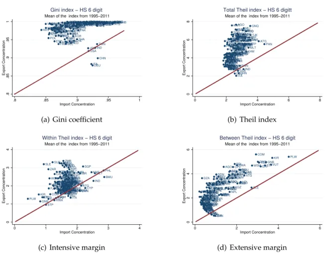
Based on net trade flows at the product level, I calculate concentration indexes for each country on all margins for each year and then take the average over the whole sample period. Because the concentration indexes used are independent of scale, the calculation on a year-to-year basis avoids the need to deflate the data. Figure 1 plots the mean export concentration against the mean import concentration for each country, together with the 45 degree line. In terms of overall concentration, Figures 1(a) and 1(b), show that the vast majority of observed levels lie above the 45 degree line indicating that exports are more concentrated than imports for almost all countries. With regard to the intensive product margin, Figure 1(c), the specialization level of exports is slightly higher than that of imports. Figure 1(d) plots the results for the extensive product margin with countries exporting fewer products than they import.
3This is a simplification, but it is reasonable as a first-order approximation because, for all countries in the sample,
this represents on average 76 percent of all merchandise imports; the median is 91 percent.
4I compute total net exports at the 6-digit product level and consider a country as an exporter of that product if net
exports are positive and an importer otherwise.
5In the appendix I present an alternative approach to account for observed intra-industry trade in the data. The
basic idea is to develop a measurement device that enables the model to characterize trade within and across products. The suggested procedure converts the product units in the model to product units in the data and allow us to examine specialization patterns based on gross trade flows. In the rest of the paper, I follow the net trade flow approach. I present the estimation and results of the alternative procedure in the appendix.
Table 1: Mean concentration indexes over 2210 country-year pairs
Gini Theil Exports (X) Theil Imports (M)
Exports Imports Extensive Intensive Total Extensive Intensive TotalMargin Margin Margin Margin
Level of 0.98 0.91 2.60 2.13 4.73 1.10 1.61 2.71
concentration
% share of overall 55% 45% 40% 60%
concentration
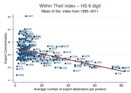
Figures 1(a) and 1(b) also reveal that some countries have higher import than export concentration (the United States, China, Germany, India and Italy). An examination of the extensive margin shows that these countries import the same number of products as they export, so the difference must stems from the intensive margin: in order words these economies have diversified export revenues and spend their import expenditure on relatively few goods. The reason for the diversification of export revenues across products is that export revenues are also diversified across countries, i.e. exporter export each of their products to many different destinations. Indeed, Figure 2 shows a significant negative correlation between export concentration and the average number of export destinations per product, pointing to complementarities in the concentration of export revenues in terms of prod-ucts and in terms of destinations.
Table 1 summarizes the sample statistics by giving the average year-by-year indexes for the 2210 country-year pairs. As implied by Figure 1, exports are more concentrated than imports on all mar-gins. With respect to overall concentration, the summary statistics reveal high levels of export and import concentration, with a Gini coefficient of 0.98 for exports and 0.91 for imports. In the case of ex-ports, the high level of concentration is due to the fact that countries export few products and hence specialization is primarily driven by the extensive margin. For imports, the decomposition favors an alternative explanation. Countries import a fairly wide range of products but concentrate their trade in the value of few products. With regard to the gap between export and import concentration, Table 1 shows that this can mainly be explained by the extensive margin. The Theil of 1.10 on the import extensive margin implies that, on average, a country net imports 33.3 percent of all products. On the other hand, the extensive Theil for exports indicates that a country net exports 7.4 percent of all products. In terms of the intensive margin, a country receives roughly 50% of its export revenues from 1% of the products it exports and spends 50% of its import expenditure on 2% of the products it imports. Overall, these results are consistent with the idea that openness to trade spurs countries to specialize in a few exporting sectors and to diversify its importing sectors.
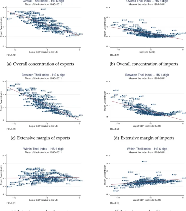
Turning to cross-country differences, the empirical evidence shows that larger economies diversify more than smaller economies. Figure 3 plots the log of the mean levels of concentration as a function of market size, including the best linear fit for all margins. Market size is measured by the log of average GDP relative to the United States (USA=0). As Figures 3(a) and 3(b) show, the overall Theil
index decreases as relative GDP increases, i.e. smaller economies specialize more. This relationship is more pronounced for exports than for imports, with an R square of 0.58 compared to 0.41. The decomposition reveals that intensive margin specialization does not vary with market size for either exports (Figures 3(e)) or imports (3(f)). The main driver of specialization differences across countries is therefore the extensive margin.The linear relationship is especially robust for the export extensive margin, with an R square of 0.75. Bigger economies are more diversified because they export more products, which is consistent with Koren and Tenreyro (2007)’s observation that larger economies are more diversified because they produce and export more products. The relationship between market size and specialization in the extensive margin of imports follows an L-shaped pattern. As an economy increases in size, it diversifies its imports, until it reaches a certain market size after which concentration is roughly equal across countries.
At this point, the key qualitative and quantitative facts have been established. First, exports are more specialized than imports. Second, concentration is driven by the extensive margin for exports and by the intenisve margin for imports. Third, the target levels of concentration are displayed in Table 1. Fourth, the cross-country patterns imply a negative relationship between market size and specialization caused by the extensive margin, i.e. larger economies export and import more products. The rest of this paper evaluates the Ricardian model’s ability to account for these stylized facts. In the next section, I present the relevant parts of theAlvarez and Lucas(2007) extension of the Eaton-Kortum framework.
3 Model
The Eaton–Kortum model is Ricardian, with a continuum of goods produced under a constant-returns technology. In this paper, I focus on theAlvarez and Lucas(2007) model and include capital as in Waugh (2010). Next, I derive the relevant theoretical predictions on the pattern of trade and evaluate the importance of the key model parameters for import and export specialization.
Consider a world economy with I countries, where each country produces tradable intermediate goods as well as non-tradable composite and final goods. Following Alvarez and Lucas (2007), I
define x = (x1, ...,xI) as a vector of technology draws for any given tradable good and refer to it as
“good x” withx2 RI+. The production of an intermediate good in countryiis defined by:
qi(xi) = xi q[kias1i a]bqmi1 b.
Technologyxi differs between goods and is drawn independently from a common exponential dis-tribution with densityfand a country specific technology parameterli, i.e. xi ⇠exp(1/li). I denote
the interest rate byri, the wage bywiand the price of the intermediate aggregate good bypm,i. The
in-termediate good sector is perfectly competitive. Producers of the inin-termediate good minimize input costs and sell the tradable intermediate good at price
pi(xi) = Bxqi[riaw1i a]bp1mib.
whereB =b b(1 b) (1 b). The continuum of intermediate input goodxgoes into the production
of the composite goodqisymmetrically with a constant elasticity of substitution(h >0)
qi =
ˆ • 0 q(x)
1 1/hf(x)dx h/(1 h).
The aggregate output of intermediate goodqi can then be allocated at no cost to the production of
final goods or can be used as an input in the production of other intermediate goods. Similarly, capital and labor can be used either to produce intermediate or final goods. Finally, consumers draw utility linearly from the final good. All markets are perfectly competitive. Since these features are not central to the implications I derived in this paper, I omit them. I refer interested readers toAlvarez
and Lucas(2007) for a full description of the model.
3.1 General equilibrium
Once a country opens up to international goods markets, intermediate goods are the only goods traded. Final goods are not traded and capital and labor are immobile between countries. Trading intermediate goods between countries is costly. We define “Iceberg” transportation costs for good
x from country ito country jby kij where kij < 18 i 6= j andkii = 1 8i. As inAlvarez and Lucas
(2007), we also consider tariffs. wij is the tariff levied by countryi on goods imported from country
j. Tariffs distort international trade but do not entail a physical loss of resources. Incorporating the trade costs, composite good producers in countryiwill buy the intermediate goodxfrom country j
pi(x) = Bmin j 2 4[r a jw1j a]bp 1 b mj kijwij x q j 3 5. (5)
Equation 5 shows that whether country i specializes in the production of good x depends on the productivity realizations, factor prices and trade costs. If country i does not offer a good at the lowest cost in the local market, the good is imported. Following Alvarez and Lucas, the resulting price index of tradable goods in countryiis
pmi = (AB) 0 B @ I
Â
j=1 0 @w b jp1mjb kijwij 1 A 1/q lj 1 C A q (6) where A = G(1+q(h 1)) is the Gamma function evaluated at point (1+q(h 1)). Next, wecalculate the expenditure shares for each countryi. Let Dij be the fraction of country i’s per capita spendingpmiqion tradables that is spent on goods from country j. Then, we can write total spending ofion goods fromjas
pmiqiDij =
ˆ
Bij
pi(x)qi(x)f(x)dx
where Bij defines the set of goods country j attains as a minimum in equation 5. Note that Dij is
simply the probability that countryjis selling goodxin countryiat the lowest price and calculated to be Dij = (AB) 1/q 0 @[r a jw1j a]bp1mjb pmikijwij 1 A 1/q lj. (7)
Equation 7 shows that in this model the sensitivity of trade between countries i and j depends on the level of technologyl, trade costsw, geographic barrierskand the technological parameterq
(re-flecting the heterogeneity of goods in production) and is independent of the elasticity of substitution
h. This result is due to the assumption that h is common across countries and does not distort
rel-ative good prices across countries. Note also that, by the law of large numbers, the probability that countryi imports from country jis identical to the share of goods countryi imports from j. In this sense, trade shares respond to costs and geographic barriers on the extensive margin: as a source becomes more expensive or remote it exports/imports a narrower range of goods. It is important to keep in mind that the number of intermediate input industries that enter into the production of the composite good is fixed. Each country uses the whole continuum of intermediate goods to produce composite goods. There are no gains from trade due to an increased number of varieties. Welfare
gains are realized through incomplete specialization. Domestic production competes with imports and countries specialize through the reallocation of resources made available by the exit of inefficient domestic producers.
To close the model, we impose that total payments to foreigners (imports) are equal to total receipts from foreigners (exports) for all countriesi
Lipmiqi I
Â
j=1 Dijwij = IÂ
j=1 LjpmjqjDjiwji (8)The previous equation implies an excess demand system which depends only on wages. Solving this system, describes the equilibrium wage for each country together with the corresponding equi-librium prices and quantities. Next, I describe the predictions for export and import concentration in both margins.
3.2 Concentration of exports and imports
In the model, the pattern of trade is established by domestic producers competing with importers to sell intermediate goods in the local market. Given the equilibrium price,p(x), and quantity,q(x), the
total amount that countryispends (c.i.f.) on imported goodx,RiM(x), is:
RiM(x) = Lipi(x)qi(x) x2/Bii
whereBii ⇢RI+is the set of goods for which countryiobtains the minimum price at home. Similarly,
domestic producers export their good to all foreign markets where they attain the minimum price. The set of exported goods is simply a the sum of goods countryi exports to any destination j, x 2
[jI6=iBji. As a result, (f.o.b.) export revenues for goodx, Ri,X(x), are given by:
RiX(x) =
I
Â
k6=i
Lkpk(x)qk(x)kkiwki x2 [jI6=iBji
Given the described pattern of trade, the concentration index for imports is identified. To show this, I decompose the overall concentration into a concentration measure for the intensive and extensive product margins. Using equation 3, the Theil index for the concentration of imports in the intensive margin can be written as:
TiMint = ˆ x2/Bii RiM(x) ¯ RiM ln ✓ RiM(x) ¯ RiM ◆ f(x)dx
In the appendix, I show that import expenditure follows a Fréchet distribution with shape parameter 1/q(h 1) and scale parameter si. Solving the integral, the intensive Theil index of imports for
countryibecomes: TiMint =ln(G(1+q(1 h))) ˆ 1 0 ln ⇣ u( q(1 h))⌘e udu (9)
whereG(.)stands for the Gamma function. Import specialization in the intensive margin is
indepen-dent of equilibrium prices, trade costs, geography and the level of technology l. It is determined
solely by preferences (i.e the elasticities of substitution) and heterogeneity in production (i.e. the degree of comparative advantage). A higher elasticity of substitution(h)increases specialization by
allowing producers in the composite intermediate good sector to better substitute cheap for expen-sive products and concentrate expenditure in these sectors. Similarly, an increase in the degree of comparative advantage(q), which corresponds to a higher variance of productivity realizations and
therefore an increase in unit price differences across goods, heightens the degree of concentration. To compute the concentration in the extensive margin of imports, note that the set of goods produced is disjoint form the set of goods imported. Consequently, we can express the share of goods imported as 1 minus the share of goods produced, (1 Dii). The Theil index for the extensive margin of
imports is equal to : TiMext =ln ✓ N NiM ◆ = ln(1 Dii) (10) where Dii = (AB) 1/q [r a iw1i a] pmi ! b/q li
and depends on the level of technology and equilibrium prices. To assess the level of specialization in exports, I simulate the model within a discrete product space in the following section. I then calculate the export concentration index for the intensive margin according to equation 3.
Having outlined the pattern of trade and the corresponding implications for the specialization pat-tern of exports and imports, the next section discusses the simulation of the model. It contains special equilibria cases designed to spell out step-by-step the main implications of the model for export and import concentration.
4 Calibration and simulation
To simulate the theoretical model, which assumes an infinite amount of goods, I "discretize" the Fréchet distribution of total factor productivity and calculate the respective trade value for each product x. Regarding the parameters of the model, we need values for a, b, g, h and q. For a, b
and g, I use the same values as Alvarez and Lucas (2007): I set the capital share to a = 0.3, the
efficient labor share in the tradable goods sector tob = 0.5 and the labor share in the production of
non-tradable final goods toa =0.75.
To calibrate the elasticity of substitution (h) and the variance of the productivity distribution (q), I
use the model’s implication on the value and the volume distribution of imports. As shown in the previous section, the distribution of import value follows a Fréchet with shape parameter 1/q(h 1).
Similarly, the distribution of the quantities imported can also be shown to follow a Fréchet with shape parameter 1/(qh). Using the fact that the Theil index for the intensive margin depends solely on the
shape parameter, I first calculate the average Theil index for import expenditure,Tint
iM =1.61, and for
imported quantities,Tint
iQ =3.58.6 Then, using equation 9, I get the corresponding shape parameters
and obtain 2 equations with 2 unknowns. The solution of the system gives an elasticity of substitution (h = 8) and a degree of comparative advantage (q = 0.10). The elasticity of substitution is high but
still in the parameter range found in the literature (seeBroda and Weinstein(2006)). The degree of comparative advantage also lies in the parameter range 0.08 to 0.15 estimated in the literature (see
Eaton and Kortum(2002)). However, compared to more recent estimates bySimonovska and Waugh
(2011),q =0.10 is rather low.
In the following subsections, I analyze import and export concentration in special cases of equilib-rium by assuming different trading schemes. Doing this builds an intuition of how taste, technology and geography determine specialization. To illustrate the impact of each factor separately, it is in-structive to start the analysis by assuming symmetric countries and introducing heterogeneity across countries at a later stage. Finally, I show that, for a particular configuration of trade costs, the Eaton-Kortum model is able to replicate the specialization patterns observed in the data.
6In addition to the dollar value of imports, BACI also reports the volume of goods imported, which are measured in
tons. To calculate the Theil index of the volume of imports, we follow the procedure applied to the import revenues. We first calculate the net volume of imports for each good and then apply equation 3. The valueTint
iQ =3.58 represents the cross-country average over the sample period.
4.1 Symmetric countries
All countries are identical. Trade costs are symmetric and set to kij = k 8 i 6= j with kii = 1 and wij = 1 8i,j. Due to symmetry, factor prices equalize across countries. The corresponding trade
share matrixDis symmetric and the(i,j)element is given by:
Di,j = (k)
1/q
1+ (I 1)(k)1/q 8i6=j and Di,i =
1
1+ (I 1)(k)1/q
In free trade,k =1, each country’s intermediate good producers specialize in a distinct set of goods
equal to the relative size of the economy and export all products produced,Dii =Dij =1/I. The
cor-responding share of imported products is 1 Dii = (I 1)/I. In this case, Ricardian specialization
forces are strongest and the gap between export and import concentration reaches a maximum.
Extensive Margin Concentration Including trade costs, the concentration index for imports equals
the share of goods countryiimports from all countries in the world and is given by:
TiMext = ln((1 Dii)) =ln(1+ (I 1)(k)1/q) ln((I 1)(k)1/q)
Concentration in the extensive margin of imports increases with trade barrierskand decreases with
the number of trading partnersI 1 and the degree of comparative advantageq. Regarding exports,
the extensive Theil index is given by the number of products exported to any destination divided by the total number of products in the world. To count the number of products exported, define the set of products exported as the union of the set of products exported to each destination,Uex =[Ij6=iBji.
Because the set of products exported to destination joverlaps with the set of products exported to destinationk, Bji\Bki 6= ∆, I apply the Inclusion Exclusion principle to avoid double counting. As
I show in the appendix, under the assumption of symmetry, the extensive Theil index of exports is given by: TiXext = ln I 1
Â
k=1 ( 1)k 1 I k ! ak ! (11) where the share of products exported tokdestinations,ak, is given by:ak = (k)
1/q
k+ (I k)(k)1/q
The concentration of exports increases with geographical barriers, the degree of comparative advan-tage and the number of trading partners. In general, a larger number of trading partners increases
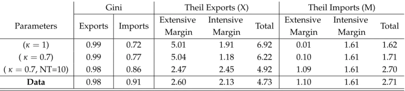
Table 2: Simulated export and import concentration indexes for benchmark parameters.
Gini Theil Exports (X) Theil Imports (M)
Parameters Exports Imports Extensive Intensive Total Extensive Intensive Total
Margin Margin Margin Margin
(k=1) 0.99 0.72 5.01 1.91 6.92 0.01 1.61 1.62
(k=0.7) 0.99 0.77 5.04 1.18 6.22 0.10 1.61 1.71
(k=0.7, NT=10) 0.98 0.86 2.47 2.45 4.92 1.09 1.61 2.70
Data 0.98 0.91 2.60 2.13 4.73 1.10 1.61 2.71
competition between production and imports in the domestic market, resulting in the production of fewer goods at home and an increase in the number of goods imported. Also, a higher number of trading partners increases competition between exporters in foreign markets, forcing countries to specialize more idn the extensive margin of exports. Impediments to trade, i.e. a reduction in k,
and a higher degree of comparative advantage,q, reduce import competition and, as a result, fewer
goods are exported and imported. Note that, in the special case of free trade, all goods produced are exported and concentration of production equals concentration of exports. Where trade costs are applied, countries export a subset of produced goods, leading to greater concentration of exports relative to production.
Intensive Margin Concentration As noted previously, import expenditure follows a Fréchet
dis-tribution and is pinned down by the elasticity of substitution (h) and the degree of comparative
advantage (q). Regarding the distribution of export revenues, the simulation shows that it depends
positively on the elasticity of substitution (h), the degree of comparative advantage (q) and
geo-graphical barriers (k). In the case of free trade, countries export all their goods to all destinations and, given that preferences are identical, export and import concentration in the intensive margin equalize.
The results presented in Table 2 show that the free trade calibration of Alvarez and Lucas(2007) is able to replicate the qualitative fact that, overall, exports are more concentrated than imports. While the simulated overall level of export concentration attains the degree of specialization observed in the data, in the benchmark free trade parametrization countries diversify excessively in imports because they import too many goods.
Next, I introduce 42 percent symmetric trade costs for all trading partners,k = 0.7. Row 3 of Table
2 shows the results. Impediments to trade reduce the number of products exported and imported and lead to an increase in extensive margin concentration for both, exports and imports. Note that
higher trade costs lower the level of intensive margin concentration for exports. Due to the increase in trade costs, only very efficient producers export and their export revenues are more evenly dis-tributed across products and trade partners. Still, the gap between export and import concentration remains substantial. The reason is that the degree of competition countries face in export and domes-tic markets is too high. In the symmetric setting the only way to reduce competition is to limit the number of trading partners. Using equation 11, the number of trading partners (NT) corresponding to the empirical Theil index is 10 (see fourth row of Table 2). Limiting the number of trading part-ners (NT) by introducing infinite trade costs for countries outside of the block reduces competition in all markets. Less competition in the domestic market increases the survival rate of local produc-ers and reduces the amount of goods imported. Note that the revenues of exporting industries are now geographically more concentrated and hence specialization in the intensive margin of exports intensifies.
To summerize, with the introduction of symmetric trade costs, the model can replicate the mean levels of concentration observed in the data. In particular, by creating trade blocks, which amounts to introducing zeros in the bilateral trade matrix, we can calibrate the model to explain the mean pattern of specialization.
4.2 Asymmetric countries
In this section I analyze the effects of cross-country heterogeneity on specialization. The empirical facts imply a negative relationship between specialization and market size. For this reason, I intro-duce heterogeneity in technologylito reflect the observed GDP differences in the data. To start with,
consider equation 8 in a free trade equilibrium:
(wiLi+riKi) =
N
Â
j=1
wjLj+rjKj Dji
which can be simplified to
li =C(wiLi+riKi)⇣wair1i a⌘ b q
(12) where C is a constant. Using equation 12, I obtain technology as a function of GDP (wiLi+riKi)
and endowments Li and Ki assuming that the inputs are chosen optimal. To calibrate l, I use GDP,
capital and population data from the Penn World table. I follow Waugh (2010) and normalize the parameters obtained forli, Liand Kirelative to the United States.
Extensive Margin Concentration Plugging in the equilibrium wage into equation 7, I get the cor-responding trade share matrixDwith the(i,j)element given by:
Dji = (wiLi+riKi)
ÂkI=1(wkLk+rkKk) 8j (13)
Equation 13 shows that under the assumption of free trade countryi’s share of the number of prod-ucts exported is equal to its level of GDP relative to world GDP. Hence, larger economies export more and import fewer products compared to smaller economies. This result is at odds with the empirical evidence. In the data, larger economies export and import more products.
4.3 Asymmetric trade costs
To reconcile the cross-country concentration differences for imports, I consider trade costs as a func-tion of either an export cost(exj) or an import cost(imi). While both types of cost can reconcile the
fact that larger countries import more goods, the following exposition focuses on the export cost.7 In this case, each country pays a country specific-cost in order to export, which is independent of the importing country j, kji = exi 8i 6= j andki,i = 18j = i. Due to asymmetric trade costs, wages and
composite good prices do not equalize. The trade share matrix is asymmetric and given by:
Dji = (AB) 1/q 0 @[wair 1 a i ]bp1m,ib pmjexi 1 A 1/q li 8i 6= j and Dii = (AB) 1/q w a ir1i a pm,i ! b/q li
Focusing on the expression for the share of goods that country i exports to country j, Dji, shows that a higher export cost reduces the fraction of the good that arrives in destination j (exi #) and
decreases the number of goods country i exports to any destination j. Solving for the equilibrium and assuming that composite good prices across countries are approximately equal, one can show that the share of goods imported is approximately:
(1 Dii) t ✓ 1 C1ex 1 q i (wiLi+riKi) ◆ (14) where C1 is a constant. Equation 14 shows that the share of goods imported increases as
country-specific export costs decerase, (∂(1 Dii)/∂exi > 0). Lower export costs allow producers to pay
higher factor prices at home and still be competitive in export markets. At the same time, higher unit costs of production reduce competitiveness at home and result in a larger share of imported goods.
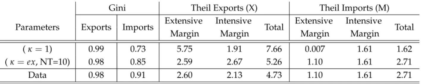
Table 3: Simulated export and import concentration indexes for asymmetric countries.
Gini Theil Exports (X) Theil Imports (M)
Parameters Exports Imports Extensive Intensive Total Extensive Intensive Total
Margin Margin Margin Margin
(k =1) 0.99 0.73 5.75 1.91 7.66 0.007 1.61 1.62
(k =ex, NT=10) 0.98 0.85 2.59 2.67 5.26 1.10 1.61 2.71
Data 0.98 0.91 2.60 2.13 4.73 1.10 1.61 2.71
Hence, an exporter-specific cost can reconcile the fact that larger economies import and export more goods.
The main difference between import costs and export costs in terms of import concentration lies in the implication for the price of tradable goods. It is possible to show that the export cost imply a near constant price for tradable goods across countries. As a result, unit cost differences between countries are predominantly driven by factor price differences. In contrast, import costs lead to large cross-country price differences, with smaller economies facing a higher tradable price level. In this case, unit cost differences are driven by factor as well as tradable goods price level differences.
Waugh (2010) provides evidence that countries have similar tradable good prices. Hence, in the
remaining analysis, I focus only on the case of the exporter-specific cost.
To summerize, the introduction of asymmetric trade costs in the form of country-specific export or import costs allows the model to replicate the import specialization pattern across countries, in par-ticular when larger economies face relatively low costs to either export or import. Waugh (2010) ar-gues that trade costs have to be asymmetric, with poor countries facing higher export costs than rich countries, in order to reconcile bilateral trade volumes and price data. While both our approaches highlight the importance of asymmetric trade costs in explaining trade data, our analysis differs. Waugh uses the Eaton Kortum model to explain bilateral trade volumes and price data whereas I look at the model’s implications for export and import specialization patterns. In this respect, the results presented in this paper provide further evidence on the importance of asymmetry in trade costs when studying trade volumes and trade patterns across countries.
Row 1 of Table 3 presents the simulation results in the case of asymmetric countries and free trade. Note that introducing technology differences increases the mean level export concentration and de-creases import concentration relative to the symmetric country case. The underlying reason is that the technology distribution is skewed towards less productive countries and these countries export
fewer goods and import more goods. Apart from these differences, the results are similar to the symmetric case.
To reconcile the empirical evidence that larger countries import more goods, I introduce country-specific export costs with larger economies facing lower export costs than smaller economies. In par-ticular, I calculate the implied export cost from equation 14 by replacing the share of goods produced at home with the extensive Theil index of imports observed in the data ,Dii =1 exp( TMExt). Row 2
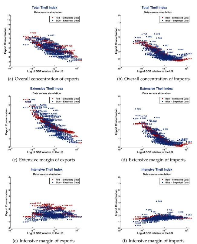
of Table 3 shows the corresponding mean concentration levels. Regarding the cross-country pattern, Figure 4 plots the simulated (in red) and empirical (in blue) concentration levels against GDP for both margins. The figures show that country-specific export costs in combination with technology and endowment differences can replicate the cross-country evidence on all margins.
In the previous section I analyzed special equilibrium cases to study the different factors that deter-mine specialization in the Eaton Kortum model. The key determinants are the degree of comparative advantage, the elasticity of substitution and asymmetric trade costs. However, I treated trade costs as free parameters and showed that, for a particular configuration of trade costs, the model is able to reproduce concentration levels for the mean as well as the cross-country specialization pattern for both exports and imports. In the next section, I estimate trade costs and technology parameters based on bilateral trade shares using the model’s structure and check whether, for given trade shares, the model is able to generate the observed specialization pattern in the data.
5 Estimating trade costs from bilateral trade shares
The starting point for the estimation of technology and trade costs is a structural log-linear “gravity” equation that relates bilateral trade shares to trade costs and model’s structural parameters. To derive the relationship, I simply divide each country i’s trade share from country j, see equation 7, by countryi’s home trade share. Taking logs yieldsI 1 equations for each countryi:
log ✓D ij Dii ◆ =Sj Si+1 q log(kij) + 1 qlog(wij) (15)
in whichSirepresents the structural parameters and is defined asSi =log([ra
iw1i a] b/qpmi(1 b)/qli).
In order to estimate the trade costskand technologylimplied by equation 15 I use data on bilateral
trade shares across 130 countries. I follow Bernard et al. (2003) and calculate the corresponding bilateral trade share matrix as the ratio of total gross imports of countryifrom countryj, Mij, divided by absorptionAbsi
Dij = AbsMij i.
Absorption is defined as total gross manufacturing output plus total imports, Mi, minus total ex-ports,Xi. To compute absorption, I use gross manufacturing output data from UNIDO.8 Combined
with trade data from BACI, I get the expenditure share, Dij, which equals the value of the inputs consumed by countryiand imported from countryjdivided by the total value of inputs in country
i. Note that instead of focusing on a particular year, I compute the expenditure share for each year of the period 1995 - 2011 and take the average expenditure share over the sample period.9
In total, there are only I2 I informative moments and I2 parameters of interest. Thus, restrictions
to the parameter space are necessary. To create them, I followEaton and Kortum(2002) and assume the following functional form of trade costs.
log kij =bij+dk+wij+exj+eij
Trade costs are a logarithmic function of distance (dk) a shared border effect between countryiand j
(bij), a tariff charged by countryito countryjand an exporter fixed effect (exj). Tariff(wij)represents
the weighted average ad valorem tariff rate applied by countryito country j. The distance function is represented by a step function divided into 6 intervals. Intervals are in miles: [0, 375); [375, 750); [750, 1,500); [1,500, 3,000); [3,000, 6,000); and [6,000, maximum]. eij reflects barriers to trade arising
from all other factors and is orthogonal to the regressors. The distance and common border variables are obtained from the comprehensive geography database compiled by CEPII.
To recover technology, I follow Waugh (2010) and use the estimated trade costs, ˆk, and structural
parameters, ˆS, to compute the implied tradable good prices, ˆpm, by rewriting equation 6 in terms of
ˆ S: ˆ pmi = (AB) I
Â
j=1 eSˆj kˆijwij 1/q ! qFrom the obtained prices and the estimates ˆSi, I get the convolution of wages and technology, log(wi b/qli).
8Details are provided in the appendix.
9The resulting sample consists of 130 times 129 potential observations if each country trades with all other countries.
In our sample the total number of observations is 15904 implying a small number of zeros in the bilateral matrix. I conduct a robustness test where I estimate the model with the Poisson estimator proposed bySilva and Tenreyro(2006). The results are similar and are available upon request.
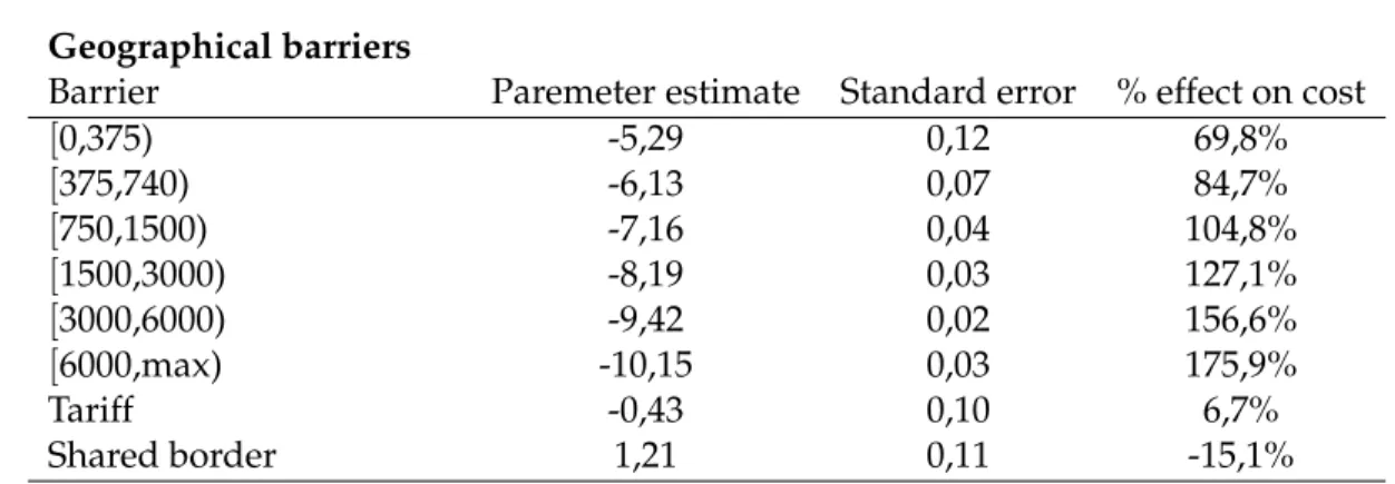
Table 4: Estimation Results Summary Statistics
Observations TSS SSR R2
7952 2,22E+05 4,08E+04 0.82
Geographical barriers
Barrier Paremeter estimate Standard error % effect on cost
[0,375) -5,29 0,12 69,8% [375,740) -6,13 0,07 84,7% [750,1500) -7,16 0,04 104,8% [1500,3000) -8,19 0,03 127,1% [3000,6000) -9,42 0,02 156,6% [6000,max) -10,15 0,03 175,9% Tariff -0,43 0,10 6,7% Shared border 1,21 0,11 -15,1%
Then, given the bilateral trade shares, Dij and the balanced trade condition in equation 8, I follow
Alvarez and Lucas (2007) and use the relationship between factor payments and total revenue to
calculate equilibrium wages.10
wi = (1 1s f i)Li ! I
Â
j=1 Ljwj(1 Fsf j) j Djiwji !wheresf iis the share of labor in the production of final goods
sf i = g(1 (1 b)Fi)
(1 g)bFi+g(1 (1 b)Fi)
andFiis the fraction of countryispending on tradable goods net of tariff expenses.
Fi=
I
Â
j=1
Djiwji
The obtained equilibrium wages together with tradable good prices, determine the implied technol-ogy levels ˆlfor each country given the structural estimates of the gravity equation.
Table 4 summarizes the regression outcome of the gravity equation. In terms of fitting bilateral trade flows, I obtain an R2 of 0.82, which is slightly lower than theR2 of 0.83 reported by Waugh.
10Given factor endowments and optimal factor choice, the interest rates equals:r
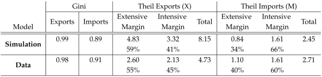
Table 5: Simulated concentration level with exporter fixed effect
Gini Theil Exports (X) Theil Imports (M)
Exports Imports Extensive Intensive Total Extensive Intensive Total
Model Margin Margin Margin Margin
Simulation 0.99 0.89 4.83 3.32 8.15 0.84 1.61 2.45
59% 41% 34% 66%
Data 0.98 0.91 2.60 2.13 4.73 1.10 1.61 2.71
55% 45% 40% 60%
The coefficients obtained for trade costs are consistent with the gravity literature, where distance and tariffs are an impediment to trade. The magnitudes of the coefficients reported in Table 4 are similar to those inEaton and Kortum(2002) and in Waugh(2010), which consider a similar sample of countries without tariffs. The overall size of the trade costs in percentage terms are similar to those reported inAnderson and Van Wincoop(2004).
Next, I feed the model with the estimated trade costs and technology levels.11 Table 5 shows the
mean concentration levels for the simulated countries. The results show that the calibrated model replicates the fact that countries are more specialized in exports than in imports on all margins. However, the levels of export concentration are almost twice as high as the ones observed in the data: mean export (import) concentration on the extensive margin is 4.83 (0.84) compared to 2.60 (1.10) in the data. This implies that, in the simulated model, countries export (import) 0.8 (43.2) percent of the product space compared to 7.4 (33.3) percent in the data.
Figure 5 plots the corresponding cross-country pattern for simulated and empirically observed centration levels against the log of GDP. The model replicates the empirical pattern with export con-centration decreases as market size increases. However, the simulated concon-centration levels in the extensive margin are too high, particularly for smaller economies. Countries specialize excessively in the number of products exported. On the import side, the calibrated model is unable to replicate the L-shaped relationship between market size and concentration: indeed, the relationship does not follow any particular pattern. However, the simulated countries tend to import more goods than in the data. With regard to the intensive margin, Figures 5(e) and 5(f), the results show that, in line with the data, the model predicts no relationship between concentration and market size. To summerize, the calibrated model is able to replicate the qualitative pattern for exports but produces relatively high levels of concentration compared to the data, particularly for the extensive margin.
5.1 Discussion of results
A potential explanation for the excessive export concentration lies in the underlying productivity distribution. While the model reproduces the bilateral trade volumes, it fails to capture the underly-ing distribution of trade volumes across products. To shed light on why countries trade in too few products, I follow Haveman and Hummels(2004) and plot the empirical and simulated density of the number of exporters and importers per product.12 Figure 6 shows the results. The simulated
countries export their goods to too many destinations. The assumed productivity distribution gen-erates producers are so efficient that even firms facing high trade costs can sell their products to numerous destinations around the world. As a consequence, the number of exporting countries per product is small. In the data (in blue) more than a third of the products are exported by 25 or more countries. In the simulation (in red) no product is exported by more than 25 countries. With regard to imports, Figure 6(b) shows that, contrary to exports, the simulated distribution of the number of countries importing a product is closely related to the empirical one.
To investigate why the model is not able to reproduce the cross country pattern of the number of products imported, we compare import expenditure and import product shares. The product share,
pi, is defined as the number of products imported, Ni,M, divided by the total number of potential
goods,N, i.e. number of HS codes:
pi = Ni,M
N (16)
and the expenditure share,mi, equals the total value of imports,Mi, divided by domestic absorption,
Absi.
mi = AbsMi
i (17)
Expenditure shares are used to calibrate trade costs while the import product share defines the ex-tensive Theil of imports. Note that the model implies that these two are equal but empirically they are not, see Figure 7.
One potential reason could be that countries differ in the number of intermediate goods used in pro-duction. When calculating the share of goods imported, I divide the total number of net products imported by the total number of HS codes, which is common to all countries. If countries do not
12To get the empirical distribution of the number of exporters and importers per product, I count for each HS code the
number of countries thatnetexport ornetimport the product. Similarly, the model implied distribution represents the number of exporters and importers for each simulated product.
make use of all tradable goods (for example they do not have the underlying technology to use a particular intermediate good), then the calculated import product share for these countries is down-ward biased. Ethier(1982) argues that larger economies use a higher number of intermediate goods because of increasing returns to scale in the production process of the final good. To shed light on the potential impact of market size on the number of intermediate products in the economy, we impose equality between product shares and expenditures shares, (pi =mi). Given this assumption, we can
rewrite this equation as:
Mi
Ni,M =
Absi
N (18)
implying that the average per product import expenditure equals the average per product tradable expenditure. Since the number of tradable goods is the same for all countries, we expect that the elasticity of the average per product import expenditure with respect to absorption is 1. Figure 8 reveals a strong positive correlation with anR2 =0.84 and an elasticity of 0.6, significantly different
from 1. Ethier’s argument that larger economies have a higher degree of specialization and use a larger number of intermediate inputs in the production of tradable goods can explain why the elasticity is less than 1. In this case, the number of tradable goods would be country specific and increases with the size of the tradable sector.
Non-homothetic preferences may represent an alternative explanation for the fact that some coun-tries spend, on average, relatively more on few imported goods. Note that, according to equation 18, the ratio of per product import expenditure to per product tradable expenditure should be one. This result relies on the assumption of homothetic preferences. Figure 9 plots the log of the ratio against the log of GDP per capita. The figure shows a negative correlation of -0.67 with anR2 =0.23.
This evidence is consistent with non-homothetic preferences, where poorer countries spend more per imported good than rich ones.
6 Robustness
6.1 Alternative classification schemes
This section addresses concerns about robustness of the observed empirical concentration indexes. In particular, the level of disaggregation as well as the chosen classification scheme may affect the empirical concentration measures and the decomposition of the intensive and extensive margins. For this reason, I re-calculated the concentration indexes for both margins using (1) 5-digit SITC product codes and (2) 6-digit NAICS codes instead of the 6-digit HS codes. The advantage of the NAICS
and SITC classification system is that the products are grouped according their economic function as well as their material and physical properties, rather than for tariff purposes as in the HS system. Table6shows the calculated concentration indexes based on SITC and NAICS classification and their correlation with respect to HS based concentration indexes. The qualitative estimates for all classifi-cation are very similar: exports are more concentrated than imports; concentration is driven by the extensive margin for exports and by the intensive margin for imports; and in terms of cross-country evidence, larger countries import and export more goods. Strikingly, the L pattern of the extensive margin also appears when the SITC and NAICS classifications are used. Differences between the various classification schemes appear in the levels of import concentration. The reason for this is that the SITC and NAICS classifications comprise a much smaller number of codes than the HS sys-tem (2,442 and 460 codes repsectively for SITC and NAICS, versus 4,529 for the HS syssys-tem). Overall, however, the high correlation between the different classification standards shows that the results are robust to the classification system.
6.2 Intra-industry trade
In this section I address the discrepancy of the product space in the data and the model caused by intra-industry trade. In the main part of the paper I established a correspondence between the model and the data by netting out within product trade. This approach leaves out valuable information and may bias the results. In an alternative approach, I deal with intra-industry trade by developing a “measurement device” that enables the model to characterize intra- and inter-industry trade. The basic idea is that, in reality, the true state of the world is indeed Ricardian, i.e. varieties are in fact products, but the data are not sufficiently disaggregated to capture the true number of products. Instead, these “Ricardian products” are aggregated into sectors according to a classification scheme, i.e. HS codes. The suggested procedure converts the measurement of product units in the model to product units in the data and allows us to examine gross trade flows. Because the classification scheme is unobserved, I assume that varieties are randomly assigned an HS code following a Poisson process. Using the structure of the model, I can then estimate the Poisson parameter and characterize the “measurement device”. I obtain a value of 0.94 for the Poisson parameter implying that, on average, one “Ricardian product” is equivalent to one HS product category. Based on this result, I group simulated Ricardian products randomly into artificial HS codes and calculate the implied concentration indexes. The results, presented in detail in the appendix, show that this approach produces similar results to the net trade flow approach.
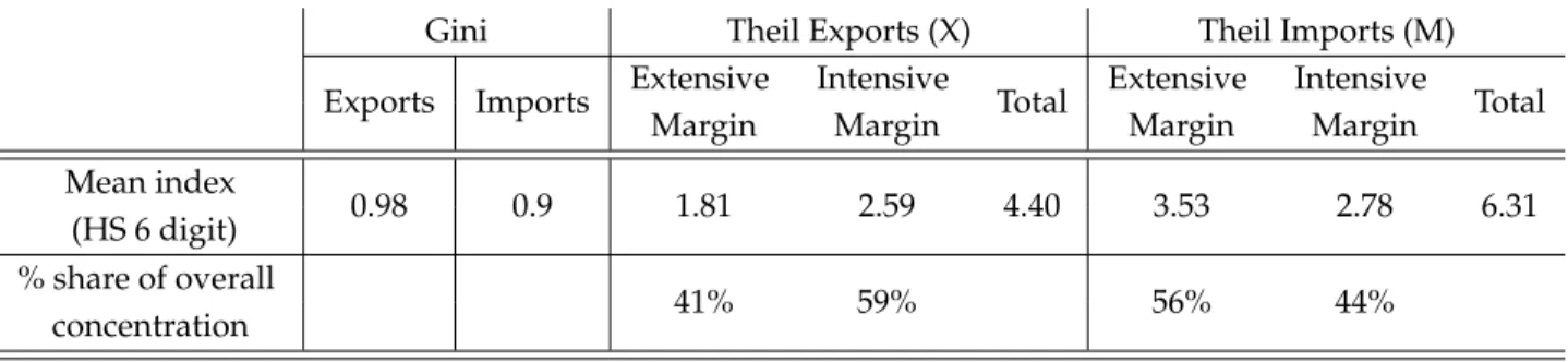
Table 6:Mean concentration indexes for gross trade flows based on the Armington assumption: 130 countries
Gini Theil Exports (X) Theil Imports (M)
Exports Imports Extensive Intensive Total Extensive Intensive Total
Margin Margin Margin Margin
Mean index 0.98 0.9 1.81 2.59 4.40 3.53 2.78 6.31 (HS 6 digit) % share of overall 41% 59% 56% 44% concentration
6.3 Implications of alternative trade models
Finally, I want to compare my analysis to alternative trade models, in particular, to monopolistic com-petition models based onKrugman(1980), and Armington models based onAnderson and Van Win-coop(2003). The key difference with respect to the Ricardian model is that in the alternative models, tradable goods are differentiated by location of production. Applying this definition of the product space to the data implies that each country is the sole producer/exporter of an HS code and demands all country-product combinations. Hence, the number of potential goods exported is 4,529 and the number of potential goods imported is 4,529 times 129 trading partners.
Table 6 presents the corresponding concentration indexes. The results show that, contrary to the findings of my model, countries are more specialized in imports than in exports and the extensive margin drives the import concentration. The extensive Theil of imports implies that the average country imports only 17121 products (around 3 percent) out of the 4529 times 129 available products. This suggests that the empirical implications used to evaluate a model depend on the definition of a product, i.e. Armington assumption versus perfect substitutes as in the classical models of comparative advantage. While it is certainly possible to produce the results in Table 6 using a model based on the Armington assumption, the underlying mechanism to generate specialization will be very different.13 In this paper, the analysis is based on the assumption that foreign varieties are
perfect substitutes for domestic ones. One motivating observation is that theGrubel and Lloyd(1975) index of 0.19 indicates that the majority of the trade flows are inter-industry (81 percent) rather than intra-industry. However, I cannot reject these alternative hypotheses for the observed concentration patterns and would like to pursue them in future research.
13For example by introducing fixed trade costs (seeRomer(1994)) or declining marginal utility of varieties (see