2004 Kluwer Academic Publishers. Manufactured in The Netherlands.
An MTIDD Based Firewall
Using Decision Diagrams for Packet Filtering
MIKKEL CHRISTIANSEN and EMMANUEL FLEURY {mixxel;fleury}@cs.aau.dk
BRICS, Department of Computer Science, Aalborg University, Fredrik Bajersvej 7, 9220 Aalborg OE, Denmark
Abstract. This paper explores the use of Multi-Terminal Interval Decision Diagrams (MTIDDs) as the central structure of a firewall packet filtering mechanism. This is done by first relating the packet filter-ing problem to predicate logic, then implementfilter-ing a prototype which is used in an empirical evaluation. The main benefits of the MTIDD structure are that it provides access to Boolean algebra over filters, effi-cient classification time, and a compact representation. Results from the empirical evaluation shows that MTIDDs are scalable in terms of memory usage: a 50,000 rule filter requires only 3MB of memory, and ef-ficient for packet classification: it is able to handle more rules than the schemes it was compared to without causing a degradation in performance.
Keywords:packet classification, firewall, decision diagrams
Abbrreviations:IDD – Interval Decision Diagram; MTIDD – Multi-Terminal Interval Decision Diagram; BDD – Binary Decision Diagram; MTBDD – Multi-Terminal Binary Decision Diagram.
1. Introduction
The Internet firewall is one of the key technologies used by network administrators for controlling access to a network. The main reason for its success is that the firewall allows filtering of traffic entering and exiting the protected network at a single centralized point. A central mechanism of the firewall is the packet filter, which decides what packets to pass through the firewall using a filter specification. Filter specification consists of a set of rules describing which policy to apply on which packet, based on the values in the packet header fields. In this paper we focus on the packet filtering mechanism, and in particular on how packet filters can be improved in terms of performance.
The primary aspect of a packet filter is the issue of packet classification which has been subject of study [Lakshman and Stiliadis, 14; Gupta and McKeown, 10; Feldmann and Muthukrishnan, 9; Singh et al., 17; Rovniagin and Wool, 15]. The reason being that the ability to classify packets plays a central role in firewalls and routing, for instance.
The requirements of the packet classification scheme differs from one application to the other. Issues mainly range from classification speed, size of the representation of the rule set and complexity of the algorithm building the representation of the rule
set. One example is packet forwarding on Internet routers, where it is essential that the classification scheme can handle frequent updates of the rule set. Firewalls, on the other hand, may classify packets using more header fields, than the router, but updates occur less frequently.
The main contributions of the work presented in this paper is a packet classification scheme, that is well suited for use in firewalls, and an empirical evaluation through a prototype implementation. This paper does not address issues such as stateful inspection and application level filters.
The central idea of the packet classification scheme presented in this paper is to transform a traditional rule based representation of a packet filter into a Boolean ex-pression represented as a decision diagram, similar to the approach presented in [Hazel-hurst, 11]. However, rather than using the widely known Boolean Decision Diagrams (BDDs) [Bryant, 7] like in [Hazelhurst, 11] as foundation for the presented scheme, we use the less explored Interval Decision Diagrams (IDDs) [Strehl and Thiele, 19]. IDDs operate on integer ranges rather than Booleans thus providing the access to efficient classification of packets on generic CPUs. The main characteristics of the IDD based scheme can be summarized as follows:
• Access to Boolean algebra over filters. This simplifies the description of algorithms used in the scheme because we can use well understood operations like comparison, union and intersection. For instance, as we shall see later, describing the transfor-mation between a filter specification and the actual representation can be expressed using Boolean algebra over filters.
• Compact representation and scalability. Decision diagram structures are optimized in space independently of the number header fields used in the specification.
• Efficient classification complexity. Namely, O(m·logr), wheremis the number of fields andris the maximum range of the fields.
• Static representation of filters. The algorithm for building the representation has polynomial complexity, therefore the scheme may not be applicable in firewalls that require frequent updates.
Moreover, we propose an extension from IDDs to MTIDDs that allows us to eval-uate a packet header against several IDDs simultaneously with no loss of efficiency. This gives the possibility of using any number of exclusives actions (policies) or non-exclusives actions to be performed on the packets.
In the following, we first describe background and related work. Section 3 de-scribes our model of packet filtering. Section 4 continues by introducing IDDs and showing how we can represent filters using IDDs. Section 5 describes the overall archi-tecture of a firewall using decision diagram based packet filters. Followed, in section 6, by an empirical evaluation where the scheme is studied under a worst case scenario. Finally, section 7 states conclusions and describe future work.
2. Related work
Several algorithms for packets classification on multiple fields for software imple-mentation on generic CPUs have been proposed in recent time [Begel et al., 4; Feldmann and Muthukrishnan, 9; Srinivasan, 18; Baboescu and Varghese, 3].
Begel et al. [4] proposes a fully general packet filter framework. Filters are speci-fied in a declarative predicate language, compiled into a flow-graph, and then optimized before being executed on a virtual machine model. Optimization is performed on the flow-graph by using redundant predicate elimination for removing redundancies and re-arranging non-optimal code sequences. The evaluation of the tool shows good perfor-mance. However, only small test cases are applied.
In [3], Baboescu and Varghese describe a scheme called Aggregate Bit Vector (ABV). The aim of the scheme is to provide scalable packet classification (100,000 rules) to handle large filters while also providing efficient classification times on generic CPUs. The scheme is an extension of the bit vector search algorithm (BV) described in [Lakshman and Stiliadis, 14].
In [11], Hazelhurst presents the idea of transforming firewall packet filters into Boolean expressions that are represented as BDDs. The paper describes an algorithm for transforming a firewall filter specified in a Cisco-like access list language into a BDD, including the handling of issues with overlapping rules. The main focus of BDDs in this paper is a tool that can analyze and test filters. A later paper by Hazelhurst et al. [12] focus on using the BDD structures for performing packet classification. The conclusion is that BDDs can improve the lookup latency on systems using dedicated hardware such as FPGAs, while they do not perform well on generic CPUs. In [2], Attar and Hazelhurst useN-ary decision diagrams for improving the lookup performance. The experimental results show that the lookup time can be significantly improved by using this method, however at the price of increased memory usage.
More recently, in [15], Rovniagin and Wool describe an algorithm called Geomet-ric Efficient Matching (GEM). Classifying packets with GEM has a time complexity of O(m·logn), wheremis the number of fields andn is the number of rules. Unfortu-nately, the worst case space complexity is O(n4). Indeed, the authors manage to show nice empirical results with this technique. In [Singh et al., 17], decision trees are widely used to classify packets. The authors introduce a new technique to split the domain of possible values into nearly optimum division.
3. Packet filtering
The problem of packet filtering is to match a packet header with a policy. This decision is based on the values in the header of the current packet and a set of rules, also called ‘filter’.
Normally filters are defined as an ordered list of independent rules. Each rule specifies both a set of headers and what policy to apply to the packet. For example, in a Cisco-like syntax, one can define the rule set represented in figure 1.
access-list 108 permit tcp any any eq www access-list 108 deny tcp any any
access-list 108 deny ip any any
Figure 1. Example of a filter in a Cisco-like syntax.
The first rule applies the policy "permit" to any TCP packet when the destination port is equal to "www" (80), if the incoming packet does not match the first rule, it is compared to the second one, which states that the filter apply the policy "deny" to any TCP packet. If, again, the incoming packet is not matched with this rule, it is compared to the last one which apply the policy "deny" to all IP packets.
The current approach is to use this filter specification strait forward. Indeed, this representation of a filter implies that the efficiency of the packet classification will be strongly related to the number of rules in the list. The worst case complexity of such algorithm is O(n·m), withnthe number of rules, mthe number of fields to check in the header. Therefore, the number of rules has a linear impact on the performance of the packet filter.
In this section, we consider a filter as a predicate logic formula on integers. This way of specifying a filter define an algebra on filters, in other words, considering filters as logic formulas, allows us to compare them and to compute the intersection or the union of two (or more) filters. Then, by using this algebra, we show that we have the same expressive power than the ordered rule-set representation. The algorithm presented here has already been described in [Hazelhurst, 11], but neither formal scheme, nor proof or evidence that all rule sets can be expressed by this mean was given.
3.1. Specifying filters as a predicate logic formula
Specifying filters as a predicate logic formula on integer variables is immediate. In order to do it right, we introduce a formal framework of the problem to be able to prove the properties we are interested in.
LetH be the set of all the possible headers, and let= {permit,deny}be the set of the policies. Aruleis given by a set of headers (η) and a policy (π):
r =(η, π ), withη⊆H andπ ∈. (1)
For example, a rule which drops packets that have the field ‘source IP’ set to 192.134.*.* and use the protocol TCP would be written:
r =(sip∈192.134.[0,255].[0,255])∧(proto=TCP),deny. (2) We define afilteras a set of rules overH ×:
ϕ =(η1, πk1), (η2, πk2), . . . , (ηn, πkn)
, (3)
By extension, we define a filter ϕ = (ηi, πki)in as a function that maps
any header h to permit and/or deny. Formally, the filtering function ϕ:H →
{permit,deny,{permit,deny}}is defined such that:
∀h∈H, ϕ(h)= {πki ∈|h∈ηi}. (4)
We say that two filtersϕ and ϕ are equivalentiff for allh ∈ H, ϕ(h) = ϕ(h). And we noteϕ ≡ ϕ. As filters are logic formulas, we can easily define the operators
¬(negation), which switchpermittodenyand vice-versa,∨(OR) which computes the union of two filters (what is accepted by one of the two filters is mapped topermit), and
∧ (AND) which computes the intersection of two filters (what is accepted by both is mapped topermit). And, finally, we call anunambiguous filter, a filter in which the set of headers(ηi)inare a partition ofH. Apartitionis defined as follows:
Definition 1. LetH be a set and(ηi)insuch that, for alli n,ηi ⊆H. Then,(ηi)in
is apartitionofH iff:
• inηi =H,
• ηi ∩ηj = ∅,∀i, j nwithi=j.
Anambiguous filtercan lead to some confusion if a packet header can be classified both inpermitand deny. In anordered filter ambiguity is avoided by letting the order prioritize among overlapping rules.
3.2. Ordered filters vs predicate logic filters
In order to prove the equivalence between an ordered filter and a predicate filter, we first have to define anordered filter.
Letψan ordered filter iffψ=(ηi, πki)inwithηi ⊂H,πki ∈for alli nand
we define an implicit orderon the rules such that:
(ηi, πi)(ηj, πj) ⇐⇒ i > j. (5)
By extension, we call anordered filterψ = (ηi, πki)ina function that maps one
header to one policy. Formally, the functionψ:H →is defined such that:
ψ(h)= {πki ∈|h∈ηi andh /∈ηj, ∀j < i}. (6)
We now state that for any ordered filterψwe can build an equivalentunambiguous
filterϕ.
Proposition 1. For any ordered filter ψ = (ηi, πki)in, we can build a filter ϕ =
(ηi, πk
i)ins.t.ψandϕ are semantically equivalent.
Proof. The proof is straightforward from the definitions and the following construction ofϕ:
πki =πki, ∀in,
ηi =ηi j <i
ηj, ∀in.
So,ϕis given by:
ϕ=(η1, πi1), η2\ {η1}, πi2 , η3\ {η1∪η2}, πi3 , . . . , ηk\ {η1∪ · · · ∪ηk−1}, πik . (7)
By construction ofϕ, we can see that this filter isunambiguousand semantically
equivalent toψ.
Therefore, from proposition 1, we deduce that our formalism is, at least, as expres-sive as the current method.
In conclusion, we managed to define filters as predicate logic formulas and intro-duce a basic algebra to manipulate them. Finally, we proved that specifying a rule-set as an ordered-list or a predicate logic formula is equivalent. We even provide an algo-rithm to derive a predicate logic specification of a filter from any ordered list. In the next section we describe an efficient data-structure for handling predicate logic formulas on integers.
4. Interval decision diagrams
As pointed out in the previous section, the packet filtering problem is equivalent to the evaluation of a predicate logic formula. Indeed, one of the most efficient data-structure, both in matter of space storage and computational time, isdecision diagrams. The most famous of these are BDDs [Andersen, 1]. Using such a data-structure to represent fil-ters have been already investigated by Hazelhurst in [Attar and Hazelhurst, 2; Hazel-hurst, 11]. Although BDDs are extremely efficient for the hardware side, they are inef-fective for the software side. Indeed, one main problem in such approach is that BDDs are based on Boolean variables only. Therefore, it is necessary to consider one bit at a time. As a generic CPU is used to consider oneword of several bits in one operation, there is an overhead on extracting bits from words. Moreover, extracting each bit re-quires specific encapsulation and cause some overhead in the memory space usage to store these structures. In order to avoid this drawback, we chose to focus on another de-cision diagram structure calledinterval decision diagram(IDD, [Strehl and Thiele, 19]). This structure allows us to perform classification on integer numbers within adomain1 (finite of infinite).
4.1. Structure of an interval decision diagrams
An IDD is adirected acyclic graph(DAG) structure in which each node corresponds to a test on an integer variable. Each outgoing edge from a node is associated to an interval within the domain of the variable attached to the node. Each edge is linked either to another node or to a Booleanterminal(TrueorFalse). AnIDD nodeis given by:
Definition 2. Letx be an integer variable defined on the domainDx ⊆Nandta
pred-icate logic formula on integer variables. We calltanIDD nodeiff one of the following hold:
• t ∈ {True,False},
• t =(x ∈I0∧t0)∨(x ∈I1∧t1)∨ · · · ∨(x ∈Ik∧tk).
With (Ii)ik a partition ofDx and (ti)ik a set of IDD nodes. We note: t = x →
(I0, t0)(I1, t1) . . . (In, tk).
We call anIDD root, an IDD node without predecessor. We say that a set of IDD nodes(ti)inis anIDDif there is only one root. Moreover, iftis an IDD node, letvar(t)
be the function which gives the integer variable tested on this node:
var(t)=
x, ift=x →(I0, t0)(I1, t1) . . . (Ik, tk),
t, ift∈ {True,False}. (8) Finally, I = ((ti)in,) is said to be an ordered IDD iff is an order on the
integer variables such that for allt ∈(ti)in witht=x→(I0, t0)(I1, t1) . . . (Ik, tk), we
havex var(ti)for eachi k.
For example, if we consider the logic formula:
(x =0∧y 3)∨(1x6∧z6)∨(x =7∧y =1). (9)
The corresponding IDD would be (see also figure 2):
t0=x →{0}, t00 [1,6], t000 {7}, t01, t00=y →[0,3], T [4,7], F,
t01=y →{0}, F {1}, T [2,7], F, t000=z→[0,6], T {7}, F.
(10)
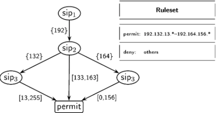
IDD structures can easily be used for describing a filter. In figure 3, we represent a very simple filter as an IDD. This example tests the ‘Source IP’ variable that we split into four subvariables (sip1,sip2,sip3,sip4) which are easier to test. Note that these IDDs do not contain any irrelevant tests and are optimum in term of operations, if we evaluate the variables in this order.
In figure 3,denyis assumed to be¬permit, as we handle only Boolean terminals. For clarity edges leading to deny are not shown in the figure.
Figure 2. Example of an interval decision diagram (IDD).
Figure 3. IDD representing a filtering rule.
4.2. Complexity of packets classification
As you can see the classification of a packet is done by simply traversing the IDD. From a theoretical point of view, it means that this algorithm has a complexity of O(m· logr), wheremis the number of fields andr is the maximum range of the fields (or the maximum number of intervals that can be in a field). This worst case complexity, when compared to the classical classification scheme (O(n·m)withnthe number of rules), appears to be independent to the number of rules. One can expect the number of rules and the number of intervals are related: the more rules you have, the more complex your IDD will be and, therefore, the more intervals you will get. However, this algorithm reduces the complexity from a linear growth to a logarithmic growth.2
It is also interesting to relate our contribution with [Rovniagin and Wool, 15]. In this paper, Rovniagin and Wool describe an algorithm classifying packets with a time complexity of O(m·logn). Their results and ours are fairly similar in terms of time complexity, but our worst case time complexity get rid of the dependence of the number 2Note that we are assuming the fact that each new rule added will produce new intervals, which is our
Figure 4. Examples of interval decision diagrams.
Figure 5. Examples of Boolean operations on IDDs.
of rules. Our scheme is bounded to the range of each field and do not depend of the number of rules in the filter.
4.3. Boolean operations on interval decision diagrams
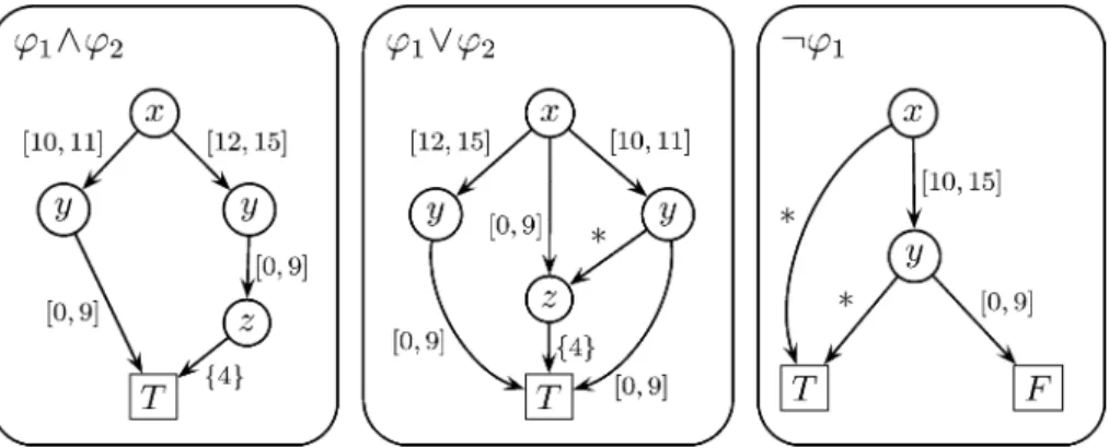
As for logic formulas, we can perform all the usual logical operations on IDDs, as nega-tion (¬), and (∧), or (∨), equivalence (≡) and so on. The advantage of this repre-sentation is that we can now manipulate the filters through the Boolean algebra. All these operators allows us to build complex operations on filters, e.g., the translation of an ordered rule-set into anunambiguousfilter. Some basic examples are given in fig-ures 4 and 5. Figure 4 represents two formulasϕ1andϕ2. Figure 5 represents the result of¬ϕ1,ϕ1∧ϕ2andϕ1∨ϕ2. The edges labeled by∗denote the complement of all the other edges. For example, if a node has four edges labeled[0,2],{9},[12,15],∗and has a range of[0,15], then∗means[3,8]and[10,11].
4.4. Optimization of interval decision diagrams
In figure 5, the result of∧ and ∨ is obviously not a strait combination ofϕ1 and ϕ2. Indeed, optimizations have been performed on the structure in order to prune redundant
nodes and subtrees. The optimization algorithm is quite simple [Strehl and Thiele, 19]. It is performed by listing each node of the IDD and applying the following optimization rules:
1. Interval merging. If two consecutive intervals of a partition lead to the same node, they are merged into one.
2. Node pruning. If a node has only one outgoing edge, the node is pruned and the ingoing edges are linked to the node pointed by the previous unique outgoing edge. 3. Subtrees merging. If two nodes are root of two identical subtrees, one subtree is pruned and all the ingoing edges coming to its root are linked to the root of the other.
When all the nodes have been processed, the input IDD to the optimization function is compared to the resulting IDD. If they are equal, a fixed-point have been reached and the optimization process terminates. If not, it takes the resulting IDD as the input and it performs the optimization function again.
This optimization algorithm is proved to always terminate (as all the rules are prun-ing an element and none is addprun-ing one). It also guaranty, that, both, the number of nodes and the depth of the IDD will be minimal for the given order3[Strehl and Thiele, 19].
4.5. Multi-terminal decision diagrams
Unfortunately, in real-life examples, when classifying network packets, you often have more than one action to perform on it. An example could be to consider the following set of actions: (PERMIT,DENY,LOG). PERMITandDENYarepoliciesand are mutually exclusive, just like we previously defined, butLOGis logging a summary of the packet to a file and can be activated in conjunction withPERMITorDENY. So, the valid set of terminals to consider will be:
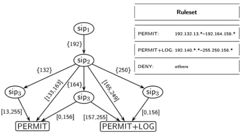
{PERMIT},{DENY},{LOG,PERMIT},{LOG,DENY}. (11) As IDDs output only Boolean variables, they cannot handle this set of terminals. In the following we extend the IDDs with more than two terminals, thus providing the possibility of using of any number of actions. This is directly derived from the multiple terminal binary decision diagrams (MTBDD [Andersen, 1]). Figure 6 represents a filter which has more than two terminals (PERMIT,PERMIT+LOG,DENY).
In the following, the terminal{DENY}is not represented and has been chosen as the default. The precise semantics is that all the intervals of a domain which are not represented in the figure leads to the default policy.
More formally, the definition is very similar to the IDD’s definition, except that we allow more than two terminals. In place of Boolean as terminal, we define a finite setT of terminals (T1, T2, . . .). Lets first define anMTIDD node.
Figure 6. MTIDD representing a filtering rule.
Definition 3. Letx be an integer variable defined on the domainDx ⊆Nandta
predi-cate logic formula on integer variables. We calltanMTIDD nodeiff one of the following hold:
• t ∈T,
• t =x →(I0, t0)(I1, t1) . . . (Ik, tk).
With(Ii)ika partition ofDxand(ti)ika set of MTIDD nodes.
The notion ofroot node is the same, but we have to extend slightly the function var:
var(t)=
x, ift=x →(I0, t0)(I1, t1) . . . (Ik, tk),
t, ift∈T. (12)
Finally, we callI =((ti)in,)anordered MTIDDiffis an order on the integer
variables such that for allt ∈ (ti)in such thatt = x → (I0, t0)(I1, t1) . . . (Ik, tk), we
havex var(ti)for eachik. For example (see figure 7):
t0=x →[0,4], t00 [5,7], t000, (13)
t00=y →[0,3], T1 [4,15], T2, (14)
t000=z→[0,1], T2 [2,+∞[, T3. (15)
Performing packet classification on MTIDD in place of IDD does not imply any complexity overhead and can be see as a strait extension of a regular IDD. But, MTIDD are no more Boolean formulas. In a matter of fact, we are computing MTIDD by com-bining IDDs.
In conclusion, we have presented an efficient data-structure to handle with predi-cate logic on integer variables (IDD), we described an algorithm to optimize in size and depth such data-structures. And, we proposed an extension from IDDs to MTIDDs that
Figure 7. Multiple-terminal interval decision diagram (MTIDD).
Figure 8. Firewall architecture.
essentially allows us to evaluate a packet header against several IDDs simultaneously with no loss of efficiency, leading to the possibility of having any number of exclusives actions (policies) or non-exclusives actions to be performed on the packets.
5. Architecture and implementation
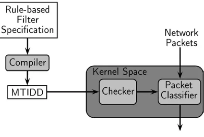
The architecture of the packet filtering prototype is shown in figure 8. The components are: the compiler, the checker, and the packet classifier. The flow of data is similar to that of writing and executing programs using a compiler: A filter is specified using a Cisco-like access list language that allows overlapping rules. A compiler translates the filter to an MTIDD using the algorithm specified in section 3.2. The compiled filter is then uploaded to a kernel-space as a temporary filter using a protocol based on Linux Netlink sockets. Once the entire filter has been constructed in space, the kernel-space module first validates the consistency of the MTIDD and then, if the validation is successful, it is used for filtering packets. In the following we look closer at issues related to the implementation of the prototype.
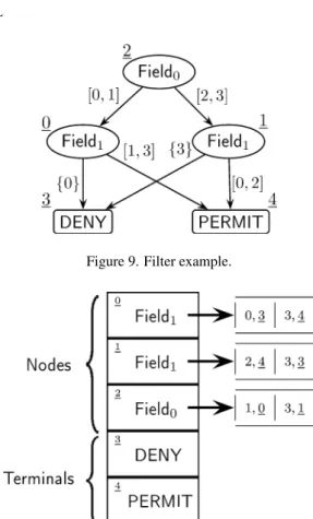
Figure 9. Filter example.
Figure 10. Organization of an IDD structure in the packet classifier.
5.1. MTIDD data-structure
The structure of the MTIDD in kernel-space is an optimized version of the adjacency-list representation of directed acyclic graphs described in [Sedgewick, 16]. The first opti-mization is that we use arrays rather than lists to improve the cache hit-rate when tra-versing the MTIDD. The second optimization minimizes the size of the data-structure. The observation is that we only need to store the upper-bound of the intervals in a par-tition. This is because the partition of an IDD/MTIDD covers the entire domainDx of
the protocol fieldx and always starts at zero. Thus, when encountering an interval we know that the lower-bound is the upper-bound of the previous interval plus one, or zero if there is no previous interval. Figure 10 illustrates the organization of the IDD shown in figure 9.
5.2. Checker
As described earlier the MTIDD passes through the Checker component that validates the MTIDD before it is taken into use. The main argument for introducing the Checker is to ensure that no matter how broken the user-space compiler is, e.g., sending broken
MTIDDs, it should not be possible to trigger a kernel crash. Thus the functionality of the Checker is to validate MTIDDs from user-space before they are used for filtering packets.
There are two main aspects to this validation of MTIDDs. The first is to ensure that the filter is an MTIDD, i.e. it contains no cycles and that all references are within the bounds of the allocated memory. This is also important in terms of performance because these tests can be safely skipped when using the MTIDD for actual packet classification. The second aspect is related to the organization of the protocol headers of the Internet protocols. An example is a filter that classifies based on the value in the TCP source port header field. We can only assume that the packets we classify are valid IP packets (see section 5.3). Therefore if we, for instance, want to read the TCP source port of a packet header, then we need to check whether the header is large enough to contain a TCP header, issues related to packet fragmentation, and whether the transport protocol is TCP. In general the following properties should always be tested before accessing transport layer headers:
• Data-length: That the amount of data received is large enough to contain a the trans-port layer protocol header.
• Fragment: That if the IP-packet is a fragment then that it is the first fragment and that it is large enough to contain the transport-layer header (TCP/UDP/ICMP). (A sender could try to avoid the transport layer filters by having fragments that are smaller than the actual TCP header.)
• IP-protocol: That the IP protocol field should match the transport-layer protocol header that is being checked.
To simplify the packet classification part of the kernel-module as much as possible, we have chosen to require that the user-space compiler includes these tests in the MTIDD before accessing transport layer headers. However since the compiler is not trustable, the Checker has to verify that the tests are actually made.
The algorithm for validating is a recursive depth-first traversal of the MTIDD. The maximum number of recursive steps is limited to the number of possible variables (max-imum depth) used in the MTIDD. This way we are sure to detect cycles and avoid over-flowing the kernel stack.
5.3. Packet classifier
By using special hooks provided by the Linux kernel it is possible to, for instance, re-ceive all IP packets being forwarded by the kernel. The actual classification of a packet consists of traversing the MTIDD, performing a binary search at each non-terminal un-til a terminal is reached. The terminal contains a policy to apply to the packet and an optional list of actions, such as logging, to perform.
The previous subsections has described the overall architecture of the prototype implementation. We believe that the main strength lies in having the main complexity
of the packet filter in the compiler that runs in user-space, therefore causing the kernel-space to be fairly simple. A consequence of this design is that the filtering policy is more static because any change requires a recompilation of the filter, but we do not see this as a problem when the application is a firewall.
6. Empirical evaluation
The relevance of using the IDD structure for packet filtering depends on whether per-formance is competitive with other algorithms for packet filtering. In the following, we describe a set of experiments that we have conducted in order to evaluate the scheme. Focus has been on two issues: space requirements and classification time.
6.1. Space requirements of the IDD structure
The worst case memory requirement of an IDD is exponential in the depth of the IDD, potentially making it unsuitable for packet filtering due to lack of scalability. However, by looking closer at the data stored in the IDD it is quite clear that exponential growth is not a realistic estimate for the actual case. In fact it is quite easy to identify often occur-ring intervals. For instance, the first bits in an IP address describes the network address, which in an IDD will be represented as intervals. Another example is the protocol field in the IP header, where only a few different values are used for specifying protocols such as TCP, UDP, ICMP, and IGMP. Two sets of experiments on size have been conducted. One on real-life filters and one on semi-synthetic filters. In the following we present the results of these experiments.
6.1.1. Real-life filters
For the first experiment we studied a set of six real-life filters. The filters are all used on production networks and manually written by professional network administrators (e.g., no automatic rule generation is used). The filtersAx are access filters from the
University routers while filtersBxare filters from a commercial organization.
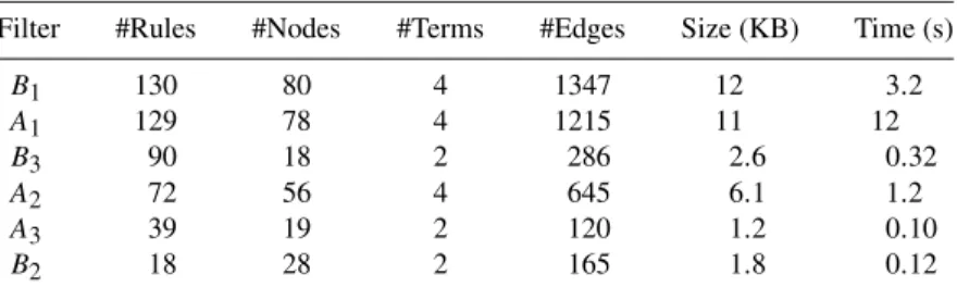
Table 1 shows the summary of the memory requirements for each of the filters. The first column two describes the number of rules in the original filter specification. Columns three and four summarizes size of resulting MTIDD, and column five shows
Table 1
MTIDD resource requirements of real-life filters.
Filter #Rules #Nodes #Terms #Edges Size (KB) Time (s)
B1 130 80 4 1347 12 3.2 A1 129 78 4 1215 11 12 B3 90 18 2 286 2.6 0.32 A2 72 56 4 645 6.1 1.2 A3 39 19 2 120 1.2 0.10 B2 18 28 2 165 1.8 0.12
the memory usage of the MTIDD structure when has been loaded into the packet clas-sification prototype. It should be mentioned that in this study we chose to split the rep-resentation of IP addresses into four variables, each representing a byte of the address separately. This may mean fewer edges but more nodes.
To some degree we see a correspondence between the number of rules in the order rule set specification and the memory requirements of the MTIDD representation. How-ever in the case ofB3a filter of 90 rules is represented with less memory than filterB2 which only has 18 rules. The reason is that filterB3has many very similar rules. Com-pile times in general acceptable except for filterA1which takes 12 seconds to compile. Further investigation is required to determine the exact cause this difference. Overall, these results are promising due to the small memory requirements.
6.1.2. Semi-synthetic filters
To provide study the growth rate of MTIDDs in a realistic setting, we have performed an experiment which allows us to look at sets that are large and yet realistic. The idea is to build filters that describe the traffic of a network backbone by letting each packet header be described by a rule specifying five values: IP protocol, and source, destination IP and ports. Using backbone traces from university network, we were able to generate rule set with sizes ranging from 10 to 50,000 unique rules. This is worst case scenario for the MTIDD based scheme because none of the rules contain intervals, only specific values.
Figure 11 and table 2 show the results of the scalability experiments. The graph in figure 11 shows the size of the MTIDD when loaded by the packet filtering prototype depending on the number of rules in the filter. Initially, we see a linear growth rate of 0.1 per rule, this drops to 0.07 between 0 and 25,000 rules. Finally, between 25,000 and 50,000 rules, the growth rate drops to 0.055. The effect is caused by new rules that
Table 2
IDD resource requirements (2.6 GHz machine). #Rules Time (s) #Nodes #Edges Size (KB)
10 0.01 28 102 2 25 0.03 77 279 4 50 0.11 128 481 7 100 0.44 232 891 14 250 3.44 542 2109 32 500 19.14 998 3952 59 1000 37.72 1884 7544 113 2500 102.1 4289 17493 261 5000 237.0 7678 31880 475 10000 571.4 13420 57417 850 25000 1832 24657 116673 1,696 50000 5221 37416 198754 2,834
produce a minimal change of an existing interval. With 50,000 rules the average size is around 60 bytes per rule. We believe that this can be minimized by more carefully designing the kernel space MTIDD structure. For instance, we could use indexing rather than pointers when referencing nodes and work on ways to reduce the redundancy of our structure.
As described earlier, the algorithm building the MTIDDs has a polynomial plexity. To show the effect of this complexity in practice, we briefly discuss the com-pilation times for transforming a rule-based filter to an MTIDD. The second column in table 2 shows the compile times for filters having sizes ranging from 10 to 50,000 rules. As we can see more realistic filters consisting of up to 1,000 rules, compiles in less than 40 seconds, which is acceptable. Larger filters with more than 10,000 rules take unac-ceptably long time to compile. However, we have not made any systematic attempts to optimize the compilation process in the current version.
6.2. Classification time
In this section, we focus on evaluating the MTIDD based packet filter by studying the performance of the MTIDD based scheme in a near worst case scenario, and compare the measured performance with that of the packet filtering algorithms currently provided on the Linux platform.
For the experiments we have chosen Linux as our test platform. The main reason for this choice is that Linux already provides two different packet filtering mechanisms, based on two different algorithms, and due to the simplicity of implementing the MTIDD based scheme as a loadable kernel module.
The two packet filtering schemes provided in Linux are: the classical packet fil-tering scheme, Netfilter [Josefsson et al., 13], and a high-performance scheme called Hipac [Bellion and Heinz, 6] which has been implemented as a Netfilter module. Net-filter performs a simple linear evaluation of the rules in the order they are stored until
a matching rule is found. Hipac uses a more advanced algorithm based on the scheme described in [Feldmann and Muthukrishnan, 9; Bellion and Heinz, 5].
The MTIDD based packet filtering scheme was implemented as a loadable kernel module. Access to packets is gained by using the hooks which a “netfilter enabled” kernel provides, thus meaning that no changes to the Linux source tree were made to implement our scheme. In addition to the kernel module, a user-space tool was written to allow MTIDDs to be uploaded to kernel memory. The data-structure for storing the MTIDD is a DAG. Filtering of packets is done by traversing the MTIDD from root to terminal and performing binary search of each partition.
For this evaluation, we are primarily interested in studying the effect on perfor-mance of a firewall with different sizes of filters and under different traffic loads. Our focus has been on keeping the experiments as simple as possible, yet allowing us to get a clear indication of whether the idea of MTIDD based firewalls is worth pursuing.
6.2.1. Setup and experimental procedure
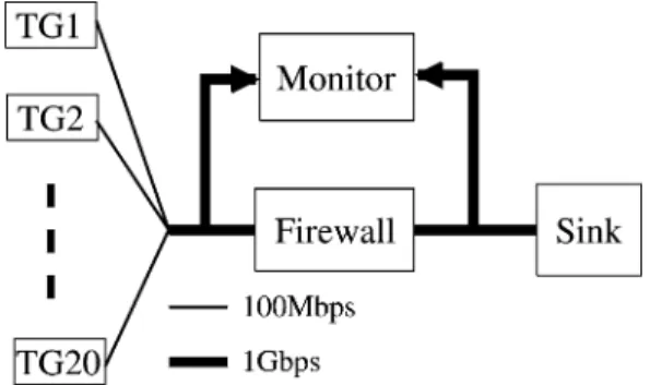
Figure 12 shows the experimental setup. At the core of the network, we have the firewall which filter traffic arriving from the traffic generators (TG1-20). The traffic is filtered and accepted traffic is routed to a sink which simply drops the incoming traffic. All nodes are connected using two switches: a Cisco Catalyst 2950 and a Cisco Catalyst 3500XL. The 2950 allows 100 Mbps links from traffic generators to be aggregated onto a 1 Gbps link, while the 3500XL switch allows the firewall to be connected to the Catalyst 2950 and the sink. To monitor the performance on the link without influencing the experiments, we use SPAN port monitoring on the catalyst 3500XL which forwards all traffic on a specific port toward a monitoring port. A machine with two gigabit interfaces is connected to the SPAN enabled ports allowing us to monitor both input and output traffic of the firewall being tested.
Each experiment consists of choosing a filtering scheme (Netfilter (Linux kernel 2.4.24), Hipac (version 0.8.0), or the MTIDD based scheme), and uploading a packet fil-ter to the chosen scheme. A traffic load is then generated using the header trace matching the installed packet filter. Packet filters and header traces were generated using a method similar to the method used for the growth rate study described in the previous section.
However, for each unique rule, we also store the unique packet header in a trace. There-fore, when replaying the header trace on a traffic generator machine we are sure that all packets are accepted by the filter and all rules are matched uniformly. This corresponds to a worst case scenario for the MTIDD based filtering scheme, because all parts of the filter is used continuously, and because each packet requires a full search of the MTIDD. In one way the generated traffic is different from the traffic described in the re-played header traces. The payload of each packet is kept fixed throughout the experi-ment. This allows us to compare the performance measured with two different filters. If we used the original payload size, then each header trace would have a different payload size distribution thus making it difficult to compare performance.
During each experiment the traffic generators run for a five minute period during which we monitor the performance of the router. Throughout the experiments, switch statistics has also been monitored to ensure that switches are not congested with traffic during any of our experiments.
6.2.2. Results
In the overall set of experiments, we have explored several combinations of input load (100, 250 and 500 Mbps). However, for clarity we only show results from experiments with a sustained input load of 500 Mbps.
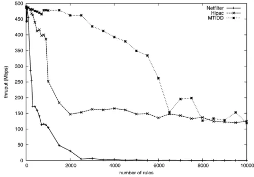
Figures 13 and 14 show the results of experiments with a sustained input load of 500 Mbps, fixed payload size of 300 bytes (∼180 Kpps (thousands of packets per sec-ond)) and number of rules ranging from 10 to 10,000. In the interval from 10 to 100 rules the performance of the packet filters are quite similar. However, both Hipac and Netfilter perform lower than expected with 25 rules. For Netfilter, throughput performance starts to degrade as the number of rules surpasses 100 rules, and continues to degrade until 2,500 rules where the throughput reaches zero. Hipac performs significantly better than Netfilter. Performance also degrades once the filter grows larger than 900 rules, how-ever at a slower rate than with Netfilter. Finally, the MTIDD based classification scheme can handle up to 3,000 rules before performance begins to degrade. Between 5,000 and 10,000 performance of Hipac and the MTIDD based scheme is quite similar. In essence, the figures clearly demonstrates the complexity difference between the approach used in Netfilter and the MTIDD based classification scheme.
Figure 15 (x-axis is now logarithmic) shows a similar set of experiments for runs with a fixed payload size of 600 bytes (∼95 Kpps). Behavior mimic the previous set of experiments except that the performance degradation occurs with larger rule sets. An interesting aspect is that, between 10–100 rules, Netfilter actually performs better than
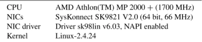
Table 3 Firewall configuration.
CPU AMD Athlon(TM) MP 2000+(1700 MHz) NICs SysKonnect SK9821 V2.0 (64 bit, 66 MHz) NIC driver Driver sk98lin v6.03, NAPI enabled Kernel Linux-2.4.24
Figure 13. Firewall throughput as a function of the number of rules (0–1000 rules). Input load is fixed at 500 Mbps load and payloads fixed to 300 bytes.
Figure 14. Firewall throughput as a function of the number of rules (0–10000 rules). Input load is fixed at 500 Mbps load and payloads fixed to 300 bytes.
Figure 15. Firewall throughput as a function of the number of rules (x-axis is logarithmic). Input load 500 Mbps and payloads are fixed to 600 bytes.
Hipac. We expect this to be due to a processing overhead of using Hipac, however further investigation is necessary to determine the exact cause. Experiments with a frame size of 1440 were also performed. But, under that load, neither of the filtering mechanisms had problems handling the 500 Mbps load. Probably due to the fairly low frame rate.
In total, these experiments shows significant performance potential of the MTIDD base packet filtering scheme. The experiments with payloads of 300 bytes is the most interesting, we were able to handle three times more rules than Hipac before reaching the performance limit with 3,000 rules. One could argue the only few firewalls will ever have filters consisting of more than 500 rules. Nevertheless, it is important to realize that even though we get similar performance with smaller rule sets, the MTIDD based scheme overall, seems to use less CPU resources than both Netfilter and Hipac, leaving more resources to other tasks allowing the use of a slower and cheaper CPU.
The conducted experiments have a limited scope and some questions remain open. For instance, the described experiments do not take into account that in a realistic setting some rules will be matched more often than other, thus allowing the approach used in Netfilter to be optimized by setting the most used rules first in the filter. In future experiments, we hope to explore performance issues related to this aspect and many others.
7. Conclusion
In this paper we have described the use of Multi-Terminal Interval Decision Diagrams (MTIDDs) as the central structure in the packet filtering mechanism of a firewall. The
work includes a mapping of traditional filter specification to predicate logic, and an empirical evaluation of the scheme, comparing it to two other schemes provided on the Linux platform.
The primary advantages of using IDDs, in a packet filtering scheme, is that an IDD describes a predicate logic expression, thus providing access to Boolean algebra over filters. MTIDDs represent the combination of several IDDs and allow us to efficiently evaluate several IDDs simultaneously. This is, for instance, relevant in cases where one can specify that packets should both be accepted and logged. A disadvantage to using IDDs and MTIDDs is that the build algorithm has polynomial complexity which can significantly impact the compile time for large filters.
The presented empirical evaluation focused on two issues: growth-rate of the size of the MTIDDs and the efficiency of the packet classification algorithm. Experiments on growth-rate showed that MTIDD based structure grows less than linearly in the num-ber of rules, when rules describe individual packet from a packet-header trace. This is a promising result, considering the fact that worst-case growth rate of an MTIDD is exponential. In addition we measured the memory requirements of real-life filters rang-ing from 20 to 130 rules. These filters consumed only marginal amounts of memory, between 1 and 12 KB.
To evaluate the packet classification algorithm, a prototype was implemented on Linux. This allowed us compare performance with two other packet classification schemes provided on the Linux platform, namely Netfilter and Hipac. The MTIDD based scheme was successful by being able to handle filters with significantly more rules before throughput of the firewall decreased.
Overall, the work presented in this paper suggests that the MTIDD structure is a strong and efficient foundation for packet filtering on firewalls.
Further work includes a more elaborate evaluation of the MTIDD based scheme, for instance by comparing it to other schemes. Also, issues on working on optimizing space requirements of the actual data-structure and minimizing compile times should be addressed as well. The prototype for Linux, called Compact Filter [Christiansen and Fleury, 8], is available for downloading.
Acknowledgments
We would like to thank the DIRT group at University of North Carolina, Chapel Hill, and in particular Felix Hernandez-Campos for providing access to relevant network traces. Furthermore, we would like to thank Jesper Sloth Christensen, Martin Dalum, and Lars Riis Olsen for making the initial implementation of the packet filter as a Linux kernel module. Finally, we would like to thank the developers of NF-Hipac: Michael Bellion and Thomas Heinz for much feedback on the implementation and menu useful discus-sions.
References
[1] H.R. Andersen,An Introduction to Binary Decision Diagrams, Lectures Notes (1997).
[2] A. Attar and S. Hazelhurst, Fast packet filtering usingN-ary decision diagrams, Technical Report, School of Computer Science, University of Witwatersrand (2002).
[3] F. Baboescu and G. Varghese, Scalable packet classification, in:Proc. of ACM SIGCOMM, San Diego, CA, USA (2001) pp. 199–210.
[4] A. Begel, S. McCanne and S. L. Graham, BPF+: Exploiting global data-flow optimization in a generalized packet filter architecture, in: Proc. of ACM SIGCOMM, Cambridge, MA, USA (1999) pp. 123–134.
[5] M. Bellion and T. Heinz, http://www.hipac.org/firewall_documentation/ packet_filter_faq.htm#l17(2003).
[6] M. Bellion and T. Heinz, Hipac (High performance packet classification for netfilter),http://www. hipac.org(2003).
[7] R.E. Bryant, Graph-based algorithms for boolean function manipulation, IEEE Transactions on Com-puters 35(8) (1986) 677–691.
[8] M. Christiansen and E. Fleury, Compact filter, http://www.cs.auc.dk/ fleury/cf/
(2003).
[9] A. Feldmann and S. Muthukrishnan, Tradeoffs for packet classification, in: Proc. of IEEE INFO-COMM, Tel Aviv, Israel (2000) pp. 1193–1202.
[10] P. Gupta and N. McKeown, Packet classification on multiple fields, in: Proc. of ACM SIGCOMM, Cambridge, MA, USA (1999) pp. 147–160.
[11] S. Hazelhurst, Algorithms for analysing firewall and router access lists, Technical Report TR-WitsCS-1999-5, Department of Computer Science, University of the Witwatersrand, South Africa (1999). [12] S. Hazelhurst, A. Attar and R. Sinnappan, Algorithms for improving the dependability of firewall and
filter rule lists, in:Proc. of the Internat. Conf. on Dependable Systems and Networks, New York, USA (2000) pp. 576–585.
[13] M. Josefsson, K. Jozsef, H. Welte, J. Morris, M. Boucher and P.R. Russell, NetFilter homepage,
http://www.netfilter.org(2003).
[14] T.V. Lakshman and D. Stiliadis, high speed policy-based packet forwarding using efficient multidi-mensional range matching, in:Proc. of ACM SIGCOMM, Vancouver, Canada (1988) pp. 203–214. [15] D. Rovniagin and A. Wool, The geometric efficient matching algorithm for firewalls, Technical
Re-port, Deptartment of Electrical Engineering Systems, Tel Aviv University, Ramat Aviv, Israel (2003). [16] R. Sedgewick,Algorithms in C, Part 5: Graph Algorithms, 3rd ed. (Addison-Wesley, Reading, MA,
2002).
[17] S. Singh, F. Baboescu, G. Varghese and J. Wang, Packet classification using multidimensional cutting, in:Proc. of ACM SIGCOMM(2003) pp. 213–223.
[18] V. Srinivasan, A packet classification and filter management system, in:Proc. of IEEE INFOCOMM, Anchorage, AK, USA (2001).
[19] K. Strehl and L. Thiele, Symbolic model checking using interval diagram techniques, Technical Re-port 40, Computer Engineering and Networks Lab., Swiss Federal Institute of Technology, Gloria-strasse 35, 8092 Zürich, Switzerland (1998).