May 2004, Volume 11, Issue 2. http://www.jstatsoft.org/
Algorithms for Spectral Analysis of Irregularly
Sampled Time Series
Adolf Mathias
ZKM - Center for Art and Media
Florian Grond
ZKM - Center for Art and Media
Ramon Guardans Medialab Madrid Detlef Seese University of Karlsruhe (TH) Miguel Canela University of Barcelona Hans H. Diebner
ZKM - Center for Art and Media
Abstract
In this paper, we present a spectral analysis method based upon least square approx-imation. Our method deals with nonuniform sampling. It provides meaningful phase information that varies in a predictable way as the samples are shifted in time. We com-pare least square approximations of real and complex series, analyze their properties for sample count towards infinity as well as estimator behaviour, and show the equivalence to the discrete Fourier transform applied onto uniformly sampled data as a special case. We propose a way to deal with the undesirable side effects of nonuniform sampling in the presence of constant offsets. By using weighted least square approximation, we introduce an analogue to the Morlet wavelet transform for nonuniformly sampled data. Asymptoti-cally fast divide-and-conquer schemes for the computation of the variants of the proposed method are presented. The usefulness is demonstrated in some relevant applications.
Keywords: spectral analysis, irregularly sampled time series, wavelets, fast algorithms, eco-nomic time series, geologic time series.
1. Introduction
Despite the vast number of methods for time series analysis, there is still a lack in manage-able methods dealing with nonuniformly sampled data. In this paper, we present a spectral analysis method based upon least square approximation, applied to different types of data. Our method is based upon assumptions similar to those of the well-known Lomb-Scargle
periodogram (Lomb 1976; Scargle 1976; Press, Teukolsky, Vetterling, and Flannery 1992;
Bretthorst 2000), and deals with nonuniform sampling. Beyond that, it has the advantage of a meaningful phase that varies in a predictable way as the samples are shifted in time, while the Lomb-Scargle periodogram was designed to compute the power spectrum. We study es-timator properties and the convergence of our results for the sample counts going towards infinity. We compare least square approximations of real and complex series and show the equivalence to the discrete Fourier transform applied onto uniformly sampled data as a special case. We analyze how constant offsets affect the obtained spectral coefficients and propose a way to deal with the undesirable side effects of nonuniform sampling.
We then reanalyze the approach with focus on weighted least square approximation and intro-duce an analogue to the Morlet wavelet transform (Chui 1992;Daubechies 1987; Holschnei-der 1995) for nonuniformly sampled data. Next, we construct a family of asymptotically fast divide-and-conquer schemes for the evaluation of the presented analysis methods. We demonstrate the functioning of our methods by applying them onto the paleoclimatic CO2
and Deuterium concentrations covering a time span of approx. 420000 years that were ob-tained from the ice core (Petit JR et al. 1999) extracted from the ice cover of Lake Vos-tok, Antarctica. The occupation with the nonuniformly sampled data presented here were the main reason for the work that lead to this publication. The paper and the data are available from http://www.nature.com/cgi-taf/DynaPage.taf?file=/nature/journal/ v399/n6735/abs/399429a0_fs.html. Finally, we apply the methods to tick data obtained on one day at the London stock exchange. Since the trade occurs at irregular times, one also has to deal with nonuniformly sampled data.
2. Spectral transforms for unevenly sampled time series
Given a time seriesx= (x0 x1 . . . xn−1) sampled at nonuniform time instantst= (t0 t1 . . . tn−1),
the approach xk = (cω sω) cos(ωtk) sin(ωtk) +ek, ∀k∈ {0, . . . , n−1} (1)
can be used to derive least square trigonometric approximations for a given angular frequency
ω. Here, ek∈Ris a zero-mean error term. In the following,P always meansPk∈K with the
index set K ={0, . . . , n−1}, and Ωt,ω denotes the matrix
cos ωt0 cos ωt1 · · · cos ωtn−1
sin ωt0 sin ωt1 · · · sin ωtn−1
.
The coefficients cω and sω can be obtained by multiplying Eq. 1 with the Moore-Penrose
pseudo-inverse (Penrose 1955),
(cω sω) = xΩTt,ω Ωt,ωΩTt,ω
−1
.
(cω sω) = X xk cosωtk sin ωtk T! P
cos2ωtk Pcosωtksinωtk
P
cosωtksinωtk Psin2ωtk
−1 = 2X xk cos ωtk sin ωtk T! n−P cos 2ωtk − P sin 2ωtk −P sin 2ωtk n+Pcos 2ωtk n2−(P cos 2ωtk)2−( P sin 2ωtk)2 (2)
and, based on that, we introduce
Pω=c2ω+s2ω, (3)
a value that will be used later in considerations about power spectra.
Lomb(1976) made similar assumptions about the nature of the analyzed data and introduced a time shiftθof the series that makes the vectors{cos (ω(tk−θ))}k∈Kand{sin (ω(tk−θ))}k∈K
orthogonal, dependent onω: X cos (ω(tk−θ)) sin (ω(tk−θ)) = 1 2 X sin 2 (ω(tk−θ)) = 1 2 X
sin 2ωtkcos 2ωθ−cos 2ωtksin 2ωθ
= 0 X sin 2ωtkcos 2ωθ = X cos 2ωtksin 2ωθ θ = 1 2ωarctan P sin 2ωtk P cos 2ωtk = 1 2ωarg X e2iωtk. (4)
The representation using arctan is the common way to express θ. Note that we silently assume it to be equivalent to the representation using arg, i.e. taking into account the signs of numerator and denominator separately and dealing with 0 in the denominator.
Applying Eq.2 onto the original time series with changed sample timestk−θ, k∈K, yields
(cω sω) = X xk cos (ω(tk−θ)) sin (ω(tk−θ)) T! 1 P cos2(ω(tk−θ)) 0 0 P 1 sin2(ω(t k−θ)) ! = P xkcos (ω(tk−θ)) P cos2(ω(t k−θ)) P xksin (ω(tk−θ)) P sin2(ω(tk−θ)) .
The absolute square value is
|(cω sω)|2= ( P xkcos (ω(tk−θ)))2 (P cos2(ω(t k−θ)))2 +( P xksin (ω(tk−θ)))2 P sin2(ω(tk−θ)) 2 ,
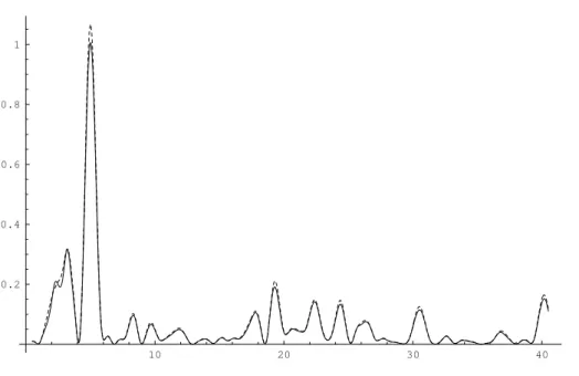
10 20 30 40 0.2 0.4 0.6 0.8 1
Figure 1: The solid line shows the absolute square result of Eq.3applied to sin(4.8t) +X0,2 ,
sampled at 400 values oftthat are uniformly randomly distributed over [0,2π). X0,2 denotes
a normally distributed random variable with mean 0 and variance 2. The dashed line shows the Lomb periodogram applied to the same data, scaled with 1821 . This factor has to be adapted for different sample counts.
Plomb(ω) = (P xkcos (ω(tk−θ)))2 P cos2(ω(t k−θ)) +( P xksin (ω(tk−θ)))2 P sin2(ω(tk−θ)) . (5)
Using the meanhxiand the varianceσ2of{xk}, the Lomb normalized periodogram is defined as Plombnorm(ω) = 1 2σ2 (P (xk− hxi) cos (ω(tk−θ)))2 P cos2(ω(tk−θ)) + (P (xk− hxi) sin (ω(tk−θ)))2 P sin2(ω(tk−θ)) ! .
The replacement of the xk with xk− hxi is one way to deal with time series with constant
offset, for which we propose an alternative solution below. This replacement is also commonly used for the unnormalized Lomb periodogram.
The amplitudes of both versions of the Lomb periodogram appear to depend on the sampling density, as can be seen in in Figure2.
In the case of a complex time seriesξ ={ξk}k∈K and an approximation by complex functions eiωt, the result is even simpler. We use the matrix Ψt,ω,
Ψt,ω = eiωt0 eiωt1 . . . eiωtn−1
to formulate the expression
20 40 60 80 100 120 140 20 40 60 80 100 120
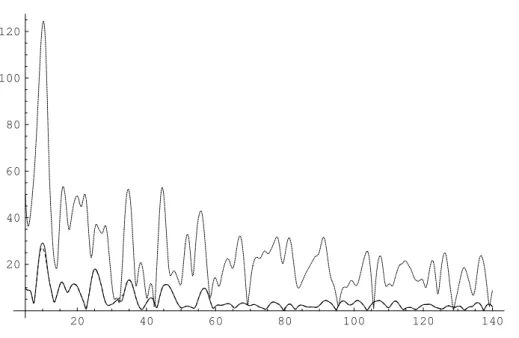
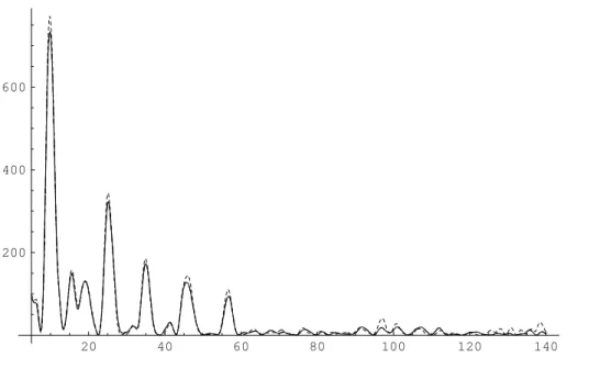
Figure 2: The solid line shows the Lomb normalized periodogram applied to the CO2 series
from the Vostok data with subtracted mean value. The densely dashed curve shows the spectrum of the same data set with odd-numbered samples removed, the widely dashed curves were obtained by doubling each sample. The abscissae show frequencies in 1/Myr.
20 40 60 80 100 120 140
200 400 600
Figure 3: The solid line shows the result of Eq.3 applied to the CO2 series from the Vostok
data with subtracted mean value. As in Figure 2, the dashed curves were obtained from of the same data set with odd-numbered samples removed and with each sample doubled, respectively. The abscissae show frequencies in 1/Myr.
20 40 60 80 100 0.2 0.4 0.6 0.8 1 1.2 1.4
Figure 4: Eq.3applied to sin 39t+ sin(39 + 2π)trandomly sampled over [0,1] with increasing density (100, 400, 2000 and 10000 points, curve plot density increasing with sample density).
analogously to Eq. 1 with a complex coefficient ζω and a vector of complex zero average error terms.
The pseudo-inverse solution yields in this case
ζω=ξΨ∗t,ω Ψt,ωΨ∗t,ω −1 = 1 n X ξke−iωtk. (7)
Using <z = 12(z+z) and =z = 21i(z−z), we rewrite the real approximation of Eq. 2 in terms of the complex approximation. Here,ζω denotes the complex approximation of the real
series{xk}k∈K,ι2ω denotes the complex approximation at frequency 2ωof the unit time series
{1}k∈K over{tk}k∈K, and <c and=cmean real and imaginary parts of a complex numberc,
respectively. We then obtain
cω+isω = 2 1− |ι2ω|2 (<ζω − =ζω) 1− <ι2ω =ι2ω =ι2ω 1 +<ι2ω 1 i = 2 ζω−ι2ωζω 1− |ι2ω|2 . (8)
In the uniform case oftk =k∆t, ∆t6= 0, k∈K ={0, . . . , n−1} and ω = nlπ∆t, l∈K\ {0},
the sumsP
cos 2ωtk and P
sin 2ωtk vanish in the real approximation given by Eq. (2), and the result is equivalent to the complex conjugate of one spectral coefficient of the discrete Fourier transform. For ω = 0, the average cω = hxi is obtained. Each term of the sum in
Eq.6 can be written as a matrix multiplication,
(cω sω) cosωtk sinωtk −sinωtk cosωtk = <xk =xk . (9)
Approximating such a uniform real-valued series with the complex approximation of Eq. 7
leaves the imaginary part undetermined, whereas the strictly real approximation of Eq.2can be interpreted as a complex equation with imaginary part set to zero,=xk = 0. Eq.2 can be
used to approximate both time series<xk and =xk of Eq.9, whereby=xk= 0, as mentioned
before, which obviously leads to cω = sω = 0. The complex approach of Eq. 9 chooses the average between the results from Eq. 2 and cω =sω = 0, which is 12(cω sω). This explains
the factor 2 in Eq.2.
In the general case of nonuniformly sampled time series, one usually estimates power spectra by means of periodograms, as for example the frequently used Lomb-Scargle periodogram (Lomb 1976; Scargle 1976; Press et al. 1992). When however phase information is desired, e.g. for the reconstruction of time series out of spectral coefficients and for comparison of signals, Eq. (2) does the job. In the sequel, we also use it for the extension of wavelet analysis onto nonuniform time series.
The amplitude of our result is invariant with respect to time shift, whereas the phase is covariant, as can be verified easily. By introducing a time shift ∆t, we have
Ωt+∆t,ω =
cosω(t0+ ∆t) cosω(t1+ ∆t) · · · cosω(tn−1+ ∆t)
sinω(t0+ ∆t) sinω(t1+ ∆t) · · · sinω(tn−1+ ∆t)
= cos ω∆t −sin ω∆t sin ω∆t cos ω∆t Ωt,ω = Rω∆tΩt,ω. (10)
The pseudo-inverse of Ωt+∆t,ω becomes then
(Rω∆tΩt,ω)∗(Rω∆tΩt,ω(Rω∆tΩt,ω)∗)−1 = Ω∗t,ω Ωt,ωΩ∗t,ω
−1
RTω∆t
and the coefficients after time shift
(cω sω)0 = (cω sω) RTω∆t.
Obviously, for the complex approximation (Eq. 7) the time shift yields
ζω0 =ζωeiω∆t.
Both the real and the complex approximation’s amplitudes are thus shift invariant, and a meaningful phase is obtained. The well-known advantage of periodograms applied to nonuni-formly sampled time series is also given here, namely their insensitivity to aliasing phenomena when the differences between theti obey a normal distribution.
We note in passing that the reconstruction of a signal from the spectral analysis of a time series requires a full matrix inverse as a consequence of the nonuniform sampling.
3. Convergence
ϕ(t) = lim n→∞→lim+0 1 n n tk t− 2 ≤tk< t+ 2 o
a generalized function describing the empirical density that the tk obey, and a real func-tion x(t) where x(t)ϕ(t) is absolutely integrable. For sequences with noncontinuous em-pirical density, e.g. tk = kmodm for a fixed m ∈ N, ϕ(t) may become infinite for some
values of t, a case which is handled by the theory of generalized functions or distribu-tions. In most cases it suffices however to consider the limits of ordinary functions, e.g.
ϕ(t) = m1 lim σ→0 1 √ πσ Pm−1 h=0 e −(t−h σ ) 2
for the previously mentioned series. Under these circumstances, we can write
lim n→∞ 1 n n−1 X k=0 x(tk) = Z ∞ −∞ ϕ(t)x(t)dt . (11)
We next consider a complex function ξ(t), where ξ(t)ϕ(t) is absolutely integrable, and a measurement error ρk obeying an independent complex symmetric distribution with zero
mean. The values ξ(tk) are identified with the ξk. The complex approximation of Eq. 7
applied toξ(tk) +ρk becomes then
lim n→∞ζω = n→∞lim 1 n X (ξ(tk) +ρk)e−iωtk = lim n→∞ 1 n X ξ(tk)e−iωtk+ lim n→∞ 1 n X ρke−iωtk = Z ∞ −∞ ξ(t)ϕ(t)e−iωtdt = Ft(ξ(t)ϕ(t)),
where (Ftf(t)) (ω) denotes the Fourier transform of f(t) with respect to the variable t at frequency ω. We note that when Ftξ(t) exists, the complex approximation converges to
Ftξ(t)∗ Ftϕ(t). The nonconstant empirical sample density ϕ(t) thus makes the complex approximation result a biased spectral estimator. The bias converges to 0 asFtϕ(t) approaches
δ0,t, i.e. components of ϕ(t) with non-zero frequency vanish. We note that
lim n→∞Var 1 n X ρke−iωtk = n→∞lim E 1 n2 X ρke−iωtk X ρke−iωtk = lim n→∞E 1 n2 n−1 X k=0 |ρk|2+ 2 n−1 X k=0 k−1 X j=0 <ρkρje−iω(tk−tj) (12) = lim n→∞ 1 nVarρk = 0,
which means that the complex approximation is a consistent estimator. The rewritten real approximation in Eq. 8becomes
lim n→∞cω+isω = n→∞lim 2 ζω−ι2ωζω 1− |ι2ω|2 = 2Ftx(t)ϕ(t)−(Ftϕ(t)) (2ω) (Ftx(t)ϕ(t)) 1− |Ftϕ(t)(2ω)|2 . (13)
We considerω 6= 0. As Ftϕ(t) approaches δ0,t, (Ftϕ(t)) (2ω) vanishes, leaving a result that,
except for the factor 2 explained above, is equivalent to the conjugate of the complex ap-proximation. Under the assumed circumstances, the real approximation thus converges to something different from the complex approximation. If ϕis symmetric, thenFtϕ(t) is real, and the real and imaginary parts ofFtx(t)ϕ(t) are scaled individually. In the general case, the real approximation converges to a complex linear combination of the complex approximation’s limit and its complex conjugate.
Since the real approximation is based on the complex approximation, it is, forFtϕ(t)→δ0,t,
an unbiased estimator. Assuming a real symmetric distribution for the error termρkin Eq.12,
we also obtain zero variance for ζω which means that the real approximation is a consistent
estimator as well.
Concluding, we can state that when the Fourier transform of the randomly sampled signal exists, i.e. the signal is a superposition of sinusoids, both the complex and the real approxi-mation converge and provide consistent and forFtϕ(t)→δ0,t unbiased estimators.
In order to study the convergence of the Lomb periodogram, we first introduce
u = lim n→∞e −iωθ = lim n→∞e −i 2arg P e2iωtk = e−2iarg(Ftϕ(t))(2ω).
Rewriting Eq. 5 and applying Eq.11, we obtain
lim n→∞Plomb(ω) = n→∞lim 1 n P xkcos (ω(tk−θ)) 2 1 n 1 n P cos2(ω(t k−θ)) + 1 n P xksin (ω(tk−θ)) 2 1 n 1 n P sin2(ω(tk−θ)) ! = lim n→∞ 1 n P xk< e−iωθeiωtk 2 1 n 1 2n P (1 +<(e−i2ωθei2ωtk)) + 1 n P xk= e−iωθeiωtk 2 1 n 1 2n P (1− <(e−i2ωθei2ωtk)) ! = lim n→∞2n 1 n P xk< ueiωtk2 1 n P (1 +<(u2ei2ωtk)) + 1 n P xk= ueiωtk2 1 n P (1− <(u2ei2ωtk)) ! = lim n→∞2n (<Ft(uϕ(t)x(t)))2 1 + (Ft(u2ϕ(t))) (2ω) + (=Ft(uϕ(t)x(t)))2 1−(Ft(u2ϕ(t))) (2ω) ! = ∞ unlessFt(uϕ(t)x(t)) = 0.
4. Wavelet transforms
We now combine the approximations derived above with a weighted least square approxi-mation to formulate a windowed transform. In our case, a weighted least square term that should be minimized with respect to (cω sω) reads
X βk2 (cω sω) cosωtk sin ωtk −xk 2 = X (cω sω) βkcosωtk βksinωtk −βkxk 2 ,(14)
whereβk2 ≡w(tk) is an appropriate weight function. We obtain the following pseudo-inverse solution for Eq.14:
(cω sω) = 2X βk2xk cos ωtk sin ωtk T! · P β2 k− P β2 kcos 2ωtk − P β2 ksin 2ωtk −P βk2sin 2ωtk P βk2+P βk2cos 2ωtk (P βk2)2−(P βk2cos 2ωtk)2−( P β2ksin 2ωtk)2 . (15)
The complex version of this is again much simpler,
ζω = P βk2e−iωtkξ k P β2 k (16) = P w(ωtk)e−iωtkξk P w(ωtk)) .
For continuous functions as well as for evenly sampled data, the Morlet wavelet transform is an instance of a weighted Fourier spectrum, whereby the window width scales withω. It uses the Gaussiane−(σωt)2with an additional scaling parameterσ as weight function.
We may now define Morlet-like wavelet transforms for unevenly sampled data by using the windowed approximations from Eq. (15) and Eq. (16). The convolution 1aR
ψ∗(b−τa )f(τ)dτ
uses the mother wavelet ψ(t), which we choose to be ψ(t) = w(σt)e−iωt in accordance with our approach. It remains to introduce a time shift. The complex case then becomes,
ζt,ω =
P
w(σ ω(tk−t))e−iω(tk−t)ξk
P
w(σ ω(tk−t))) . (17)
In order to accelerate the computation, we use a window function with compact support in time that does not employ transcendental functions,
w(t) =
(1− |t|)3+ 3|t|(1− |t|)2= 1−3|t|2+ 2|t|3, t∈[−1. . .1]
0 otherwise ,
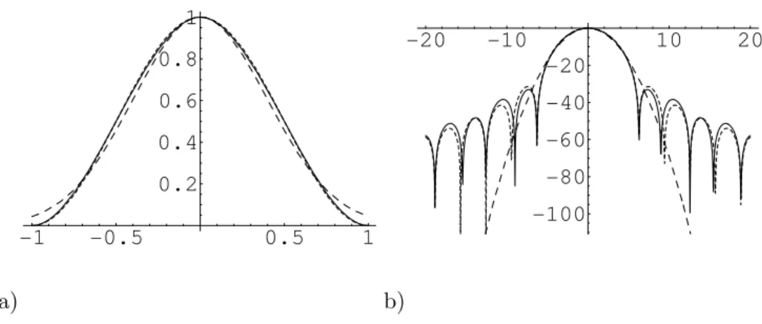
a) -1 -0.5 0.5 1 0.2 0.4 0.6 0.8 1 b) -20 -10 10 20 -100 -80 -60 -40 -20
Figure 5: Shown are (a)w(t) (solid) compared with the Hanning window (fine-dashed) and the appropriately scaled Morlet wavelet window e−πt2 (dashed), and (b) their logarithmic power spectra, measured in dB. The Hanning window andw(t) nearly coincide in (a).
This window function has a shape that is very similar to the popular Hanning window (see Figure5)
h(t) =
(1 + cos(πt))/2, |t| ≤1
0 otherwise . (18)
Its Fourier transform is
ˆ
w(ω) = 122−2 cos(ω)−ωsin(ω)
ω4 ,
and it produces comparable sideband ripples (see Figure5). The first sideband ripple is even lower than the Hanning window’s one and not substantially worse than the sideband falloff of the Gaussian’s spectrum. All three power spectra are shown in Figure5. An appropriate choice for the value ofσ is 0.05. This means that 2σ radians or πσ1 periods ofe−iωt fit into the whole support of the weight function.
In order to estimate the spectral phase differences between two complex time seriesξk, tk, k∈
0, . . . , K−1 and ηl, ul, l ∈ 0, . . . , L−1, we use the complex conjugate product of their
ap-proximations according to Eq.17,
PK−1 k=0 w(σω(tk−t))e−iω(tk−t)ξk PK−1 k=0 w(σω(tk−t)) PL−1 l=0 w(σω(ul−t))eiω(ul−t)ηl PL−1 l=0 w(σω(ul−t)) = PK−1 k=0 w(σω(tk−t))e−iωtkξk PK−1 k=0 w(σω(tk−t)) PL−1 l=0 w(σω(ul−t))eiωulηl PL−1 l=0 w(σω(ul−t)) . (19)
Since e−iωtkξk and eiωulηl do not vary with t, they can be precomputed, which accelerates the computation in comparison to Eq.17 when the result is computed with increasingly fine time resolution.
5. Fast approximation
We use the power series approximation of eit to formulate a divide-and-conquer scheme for the evaluation of Eq. 7 consisting of 4 fundamental steps described below. A fast algorithm for the real approximation that makes use of the complex approximation is given thereafter.
5.1. Complex approximation
Subdivision
In a first step, the index setK ={0, . . . , n−1}is subdivided into subsetsKh with associated τhsuch that for a given highest analysis frequencyωmax, whene−iωmax(tk−τh)is approximated
by a power series, the error is sufficiently small.
The sampling times fork ∈Kh obey −∆τ ≤tk−τh <∆τ, which is chosen as ∆τ = ωmaxc ,
i.e. a constant multiple of the period length defined byωmax(Floating point processors often
use c = π2 for computing the sine and cosine functions). The initial τ0 is chosen such that
−∆τ ≤t0−τ0, and τh+1 = 2∆τ+τh. The subdivision yields H=
l tn−1−t0 2∆τ m subsets. Precomputation
Next, for each Kh, the vector sh of the P + 1 first terms of the power series expansion of
1 n P k∈Khxke−i(tk−τh) is precomputed as sh ={sh,p}0≤p≤P = X k∈Kh xk(−iµ(tk−τh))p p! 0≤p≤P .
The factor µplays a role in the improvement of numeric accuracy. For now, we can assume
µ= 1.
Summation for a given ω
Using thesh, we now compute the spectral coefficients for 12ωmax< ω ≤ωmax.
1 n n−1 X k=0 xke−iωtk = 1 n H−1 X h=0 e−iωτh X k∈Kh xke−iω(tk−τh) = 1 n H−1 X h=0 e−iωτh X k∈Kh ∞ X p=0 ω µ p xk(−iµ(tk−τh))p p! ≈ 1 n H−1 X h=0 e−iωτh P X p=0 ω µ p X k∈Kh xk(−iµ(tk−τh))p p! = 1 n H−1 X h=0 e−iωτh P X p=0 ω µ p sh,p.
Using the fact that theτhare evenly spaced, thee−iωτhdo not have to be calculated explicitly
but can be obtained frome−iωτ0 by repetitive multiplication ofe−2iω∆τ.
Merging of s2h and s2h+1 into s0h
For the upper limit of the next frequency intervalωmax0 := 12ωmax, the power series approxi-mation has the required exactness over an interval of double length. It follows that thes2h
ands2h+1 can be combined to s0h, using the offset τh0 := 21(τ2h+τ2h+1) and size ∆τ0 := 2∆τ
belonging to the index setKh0 with−∆τ0 ≤tk−τh0 <∆τ
0 for allk∈K0
h. The index h now
runs from 0 to H0 := H
2
. The vectors of power series expansion terms s2h and s2h+1 are
combined into s0h using reexpansion:
s0h = X k∈K0 h xk(−iµ(tk−τh0)) p p! 0≤p<P = X k∈K2h xk(−iµ(tk−τ2h+τ2h−τh0))p p! 0≤p<P + X k∈K2h+1 xk(−iµ(tk−τ2h+1+τ2h+1−τh0))p p! 0≤p<P = X k∈K2h xk p X q=0 p q (−iµ(tk−τ2h))q(−iµ(τ2h−τh0))p−q p! 0≤p<P + X k∈K2h+1 xk p X q=0 p q (−iµ(tk−τ2h+1))q(−iµ(τ2h+1−τh0))p−q p! 0≤p<P = p X q=0 (−iµ(τ2h−τh0))p−q (p−q)! X k∈K2h xk (−iµ(tk−τ2h))q q! 0≤p<P + p X q=0 (−iµ(τ2h+1−τh0))p−q (p−q)! X k∈K2h+1 xk (−iµ(tk−τ2h+1))q q! 0≤p<P = p X q=0 s2h,q (−iµ(τ2h−τh0))p−q (p−q)! + p X q=0 s2h+1,q (−iµ(τ2h+1−τh0))p−q (p−q)! 0≤p<P = ( p X r=0 s2h,p−r (−iµ(τ2h−τh0))r r! + p X r=0 s2h+1,p−r (−iµ(τ2h+1−τh0))r r! ) 0≤p<P . (20)
With the introduction of ∆τ =τ2h+1−τh0 =−(τ2h−τh0), this can be further simplified:
s0h = ( p X r=0 s2h,p−r (−iµ(−∆τ))r r! + p X r=0 s2h+1,p−r (−iµ∆τ)r r! ) 0≤p<P
= ( p X r=0 ((−1)rs2h,p−r+s2h+1,p−r) (−iµ∆τ)r r! ) 0≤p<P (21) = ( p X r=0 (s2h,p−r+ (−1)rs2h+1,p−r) (iµ∆τ)r r! ) 0≤p<P (22) = bp 2c X q=0 (s2h,p−2q+s2h+1,p−2q) (−1)q(µ∆τ)2q (2q)! + i bp−1 2 c X q=0 (s2h,p−2q−1−s2h+1,p−2q−1) (−1)q(µ∆τ)2q+1 (2q+ 1)! 0≤p<P (23)
This process is repeated until either ωmax(d+1) = 12ωmax(d) passes the desired minimal analysis
frequencyω0, or the merging of adjacent subsets leaves just one subset behind (which means
that at frequencies below theωmax(d) where this occurs, the time range of the time series covers
merely a fraction of a full period of e−iωt, which is of questionable value, except forω = 0). When the number of subsets in one level is odd, the last remaining vector s(Hd)(d) is merged
with an empty one.
5.2. Real approximation
Based on the scheme for complex approximation and the complex representation of the real approximation in Eq.8, a computation scheme for the real approximation can be constructed,
cω+isω =
2 ζω−ι2ωζω
1− |ι2ω|2 .
As in Eq. 7, ζω denotes the complex approximation result for the considered time series, whereasι2ωdenotes the complex approximation at frequency 2ωof the unit time series (1. . .1)
over (t0. . . tn−1) that can be computed in a separate subdivision scheme with a few obvious
simplifications stemming from the fact that the sample values equal 1.
We note that in the real case, the sh,p are real when p is even and imaginary otherwise. In
Eq. 23, it can be seen that most of the computation steps for the merging process can be performed with purely real arithmetic, which further speeds up the computation.
5.3. Complexity considerations
We analyze the application of the fast scheme onto logarithmic and linear ranges of frequencies. In the logarithmic case, the algorithm provides the highest acceleration compared to the straighforward implementation of 7. Assuming that noct octaves of ncoeff spectral coefficients
per octave shall be computed, the following steps, each shown with their complexity, have to be performed:
• Summation forncoeff spectral coefficients in each of the noct octaves withωmax(d+1) < ω≤
ω(maxd) , 0≤d < noct: O ncoeffPH2d
,
• Merging of the sh and sh+1: O P22Hd
.
Summing everything up and applying the sum of geometric series, we obtain a total complexity of O = O nP + noct−1 X d=0 (ncoeff+ 1)P2 H 2d ! =O(P(n+ncoeffHP)).
When a linear frequency rangeωl= lωmaxL , l∈ {0, . . . , L}is desired, the number of coefficients
that can be computed with subdivision level d is 2Ld
− L 2d+1 = O 2Ld . For ω = 0, the coefficient is computed using the 0th term of thesh. Summation of the above and substitution
of geometric series yields
O =O nP + dmax X d=0 L 2d+ 1 P2H 2d ! =O(P(n+H+LH)) =O(P(n+LHP)).
5.4. Weighted complex approximation
Here, we use the Hanning window from Eq.18. We build upon subdivision and precomputa-tion steps similar to the ones described above, with
sh={sh,p}0≤p≤P = X k∈Kh xk(−i(tk−τh))p p! 0≤p≤P and jh={jh,q}0≤q≤Q= X k∈Kh (i(tk−τh))q q! 0≤q≤Q ,
whereQcan be chosen smaller thanP. We then rewrite Eq.17 as follows,
X k∈K xkw(σω(tk−t))e−iω(tk−t) X k∈K w(σω(tk−t)) = X k∈K(t) xk(1 + cos (σω(tk−t)))e−iω(tk−t) X k∈K(t) (1 + cos (σω(tk−t))) ≈ X h∈H(t) X k∈Kh
xk e−iω(tk−t)+12e−iω−(tk−t)+12e−iω+(tk−t)
X h∈H(t) X k∈Kh 1 +12eiσω(tk−t)+1 2e−iσω(tk−t)
≈ X h∈H(t) e−iω(τh−t) P X p=0 ωpsh,p+ 12e−iω−(τh−t) P X p=0 ωp−sh,p+ 12e−iω+(τh−t) P X p=0 ω+psh,p X h∈H(t) 1 +12eiσω(τh−t) Q X q=0 (σω)qjh,q+ 12e−iσω(τh−t) Q X q=0 (−σω)qjh,q
using the abbreviations ω− = ω(1− σ) and ω+ = ω(1 + σ). K(t) denotes the range
ka. . . kb of indices of samples that lie within the translated and scaled Hanning window,
i.e. σω(tka−t) < π and σω(tkb−t) < π. H(t) denotes the range of indices of subdivision
intervals that cover the Hanning window. The factorse−iω−(τh−t),e−iω(τh−t),e−iω+(τh−t) and
eiσω(τh−t) can be multiplied up iteratively from their respective start value forτha. The
pair-wise merging of the sh and jh is performed similarly to the complex approximation. It has
to be noted that the process of covering the periodic extension of the Hanning window used with precomputed sample ranges introduces small errors since the sample range boundaries almost never coincide with the window’s boundary.
6. Approximation for time series with constant offset
When analyzing time series with a constant offset, e.g. x+d(1. . .1), d∈R, using Eq. 2, we have d(1. . .1)ΩTt ΩtΩTt
−1
6
= 0 in the general case, due to the nonorthogonality of the row vectors of Ωt and the unit vector. This leads to increasingly wrong spectral coefficients for
low frequencies. We therefore compute
(cω sω dω)
cosωt0 cosωt1 . . . cosωtn−1
sinωt0 sinωt1 . . . sinωtn−1
1 1 . . . 1
= (x0 x1 . . . xn−1), (24)
by means of the pseudoinverse,
(cω sω dω) = 2X xk cosωtk sinωtk 1 T n+P
cos 2ωtk Psin 2ωtk 2Pcosωtk
P sin 2ωtk n−P cos 2ωtk 2P sinωtk 2P cosωtk 2 P sinωtk 2n −1 = 2n <ζω −=ζω hxi n 1 +<ι2ω −=ι2ω 2<ιω −=ι2ω 1− <ι2ω −2=ιω 2<ιω −2=ιω 2 −1 (25) = <ζω −=ζω hxi 0 B B @ 2−4(=ιω)2−2<ι2ω 2=ι2ω−4<ιω=ιω 2<ιω(<ι2ω−1)+2=ι2ω=ιω 2=ι2ω−4<ιω=ιω 2−4(<ιω)2+2<ι2ω 2=ιω(<ι2ω+1)−2=ι2ω<ιω 2<ιω(<ι2ω−1)+2=ι2ω=ιω 2=ιω(<ι2ω+1)−2=ι2ω<ιω 1−|ι2ω|2 1 C C A 1−|ι2ω|2−2|ιω|2+2<ι2ω((<ιω)2−(=ιω)2)+4<ιω=ιω=ι2ω .
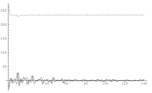
20 40 60 80 100 120 140 20 40 60 80 100 120
Figure 6: The absolute value from Eq.25 applied to the Vostok CO2series (solid) compared
with the absolute value from Eq.2applied to the CO2 series (densely dashed) and to the CO2
series with subtracted mean value (widely dashed, nearly coincident with the solid curve).
using the symbolsζω and ιω as above to denote complex approximations for the time series and the unit series. The ζω, ιω and ι2ω can be computed in divide-and-conquer schemes,
whereby the results for ιω can be reused as ι2ω in subsequent octaves.
When looking at Eqs. 1and24, it becomes obvious that at low frequencies, the approximation becomes problematic. In Figure7 which displays results down to a frequency corresponding to a third of one period over the full sample time span of 422000 years, it can be seen that the low frequency coefficients start to diverge. As a rule of thumb, we note that approximation of time series over a time span of less than half a period becomes undefined.
Looking for periodic components in a signal, we did some promising experiments with the simultaneous approximation of sinusoids with m integer multiple frequencies of a given ω0,
using the pseudoinverse solution of
(dω cω sω. . . cmω smω) 1 cosωtk sinωtk .. . cosmωtk sinmωtk k∈K =x.
It is possible to construct a divide-and-conquer scheme for these approximations as well. It becomes impracticable however to perform the matrix inversion algebraically.
20 40 60 80 100 120 140 50 100 150 200 250
Figure 7: Cosine (solid), sine (densely dashed) and constant coefficients (widely dashed) of Eq.25 applied to the Vostok CO2 series.
7. Application samples
The software accompanying this paper is written as an R module, and was developed under Linux. Besides the functions written in native R in order to provide a comprehensive sample, the real and complex spectral transform algorithms and the weighted transform, as well as their non-accelerated counterparts have been implemented in C as a loadable library. We give an overview and a couple of examples using the implemented functions here; please refer to the online documentation in R for details concerning their application and further examples. The R package is distributed as a compressed installation directory. Please use the shell command
tar xzvf nuspectral.tgz; R CMD install nuspectral
to install the package into the appropriate directories of your R installation. You may have to login as super-user first before performing the installation.
After having started R, please use
library("nuspectral")
to load the library. For the function names mentioned below and the data sets provided with the package, help pages are available that can be viewed using the R help command, e.g.
help("fastnureal")
The following functions, each operating on the time series defined by the abscissa vector X and the ordinate vector Y , are provided:
• lombcoeff(X, Y, o) computes a coefficient of the Lomb periodogram for the given circular frequency.
• lombnormcoeff(X, Y, o)computes a coefficient of the Lomb normalized periodogram for the given circular frequency.
• nurealcoeff(X, Y, omegamax, ncoeff, noctave)nurealcoeff
• nuwaveletcoeff(X, Y, t, o, wgt = cubicwgt, wgtrad = 1)computes a coefficient of the nonuniform wavelet transform in Eq.17 at the given time and circular frequency. The weight function is by default the cubic polynomial weight function shown in Fig-ure 5, and the radius beyond which the weight function is truncated to 0 is by default 1.
• nucorrcoeff(X1, Y1, X2, Y2, t, o, wgt = cubicwgt, wgtrad = 1)computes a co-efficient of the wavelet correlation of the time series given by abscissa vectors X1 and X2 and ordinate vectors Y1 and Y2 respectively.
The following functions have been implemented in C.
• nucomplex(X, Y, omegamax, ncoeff, noctave)computes the logarithmically scaled complex spectral approximation of Eq. 7 for the given maximum circular frequency, number of coefficients and coefficients per octave.
• fastnucomplex(X, Y, omegamax, ncoeff, noctave)is the accelerated version of the above according to section 5.1.
• nureal(X, Y, omegamax, ncoeff, noctave)computes the logarithmically scaled real spectral approximation of Eq. 3 for the given maximum circular frequency, number of coefficients and coefficients per octave.
• fastnureal(X, Y, omegamax, ncoeff, noctave) is the accelerated version of the above according to section 5.2.
• nurealwavelet(X, Y, omegamax, ncoeff, noctave, tmin, tmax, tsubdiv, sigma=0.1)
computes the wavelet spectrum of Eq. 17 for real Y, the given maximum circular fre-quency, number of coefficients, coefficients per octave, time interval and time subdivi-sion.
• fastnurealwavelet(X, Y, omegamax, ncoeff, noctave, tmin, tmax, tsubdiv, sigma=0.1)
computes the accelerated wavelet spectrum using the Hanning window according to sec-tion 5.4.
The data we will be using stem from
• the Vostok Lake ice drilling core (Petit JR et al.1999); the ice column extracted from a more than 3 km deep hole drilled into the antarctic ice over the huge frozen lake near the Russian Vostok research station provides invaluable information about climate, chemical composition of the atmosphere and other factors within the last 422000 years. The time series are all nonuniform, and almost none of the sample times of different series match.
• tick data from the 11. July 2001 at the London stock exchange. Given are the rates of all stocks sampled at the transaction times. Since the rates change upon trade transactions that occur more or less randomly, these time series are also sampled nonuniformly.
Distributed in R format with the package are the Vostok data series
• co2 – the CO2 content of the ice.
• ch4 – the Methane content of the ice.
• deut – the Deuterium content of the ice; the ratio of Deuterium to total Hydrogen is a proxy for the atmospheric temperature.
• o18 – the 18O (a heavy Oxygen isotope) content of the air enclosed in the ice, a proxy for the solar irradiation.
• dust – the dust content of the ice.
The stock data example has been downloaded from the internet, and has not been included into the R package because of copyright issues.
The wavelet transform diagrams below haven’t been generated with R. Some exemplary in-vocations of R functions that perform the equivalent transformations are presented, however, in the respective figure captions.
8. Summary
We have presented a way to compute spectra for nonuniformly sampled data based on least square approximation and the Moore-Penrose pseudoinverse, both for real and complex ap-proximations. The presented methods are shift-covariant in time and provide phase informa-tion. We have analyzed the correspondence of our methods with the discrete Fourier transform and the impact of constant signal offsets onto the spectral coefficients, and studied estimator properties and the convergence of our results for the sample counts going towards infinity. We further have introduced weighted versions of these spectral transforms that provide wavelet transforms for nonuniformly sampled data.
As a most remarkable result, we have presented asymptotically fast algorithms for the com-putation of the real and complex spectral analysis, which makes our methods comparably as powerful as the fast Fourier transform. These fast and robust methods to evaluate the spectral signal in time series open up new possibilities for real-time applications of increasing importance in many fields, e.g. in medicine, physiology as well as video and audio process-ing. The methods have also been applied in an interactive work of art where the user can explore animated 3D renderings in image and sound of a spectral analysis of the Vostok data. Our methods also promise to be useful for reconstruction and interpolation of missing and distorted data. The potentiality of our methods has been hinted by the presented relevant applications.
Future work will include an improvement of the numerical basis of our fast algorithms, and the development of other fast algorithms based on the presented scheme.
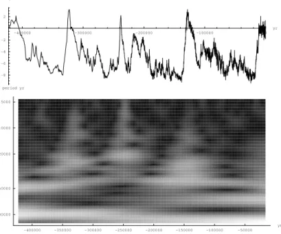
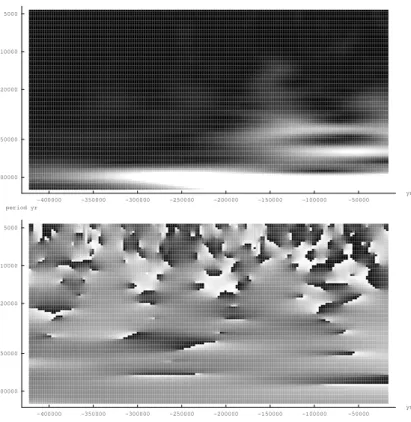
-400000 -300000 -200000 -100000 0 yr 200 220 240 260 280 300 ppmV -400000 -350000 -300000 -250000 -200000 -150000 -100000 -50000 yr 5000 10000 20000 50000 100000 period yr
Figure 8: The Vostok CO2 series and the absolute square value of Eq. 17 applied to it and
displayed as intensity. The prominent peak at a period of approx. 100000 years appears to have a diminishing frequency. The R table whose absolute square value has been visualized was obtained with
nurealwavelet(co2[[2]],co2[[4]],0.0015,100,20,0,420000,10000) -400000 -300000 -200000 -100000 0 yr -8 -6 -4 -2 2 °C -400000 -350000 -300000 -250000 -200000 -150000 -100000 -50000 yr 5000 10000 20000 50000 100000 period yr
-400000 -350000 -300000 -250000 -200000 -150000 -100000 -50000 yr 5000 10000 20000 50000 100000 period yr -400000 -350000 -300000 -250000 -200000 -150000 -100000 -50000 yr 5000 10000 20000 50000 100000 period yr
Figure 10: The absolute value and the phase of Eq. 19 applied to the Vostok CO2 and
Deuterium series, showing an interdependence of the two values over time and frequency. Medium gray encodes in-phase, white and black encode opposite phase, light gray indicates that the CO2 value is ahead of the Deuterium value. Further studies of results of this kind
could provide a deeper understanding of climatic mechanisms. The R table whose absolute square value and phase have been visualized was obtained with
nurealwavelet(co2[[2]],co2[[4]],0.0015,100,20,0,420000,10000) *
35000 40000 45000 50000 55000 sec 440 445 450 455 pound 30000 35000 40000 45000 50000 55000 sec 1000 2000 5000 10000 20000 period sec
Figure 11: Tick data for British Telecom on 11/07/2001 at the London stock exchange and the absolute value of Eq.17 applied to it. The abscissa values are in seconds past midnight.
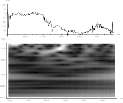
35000 40000 45000 50000 55000 sec 346 348 350 352 354 356 358 pound 30000 35000 40000 45000 50000 55000 sec 1000 2000 5000 10000 20000 period sec
Figure 12: Tick data for British Airways on 11/07/2001 at the London stock exchange and the absolute value of Eq.17 applied to it. The abscissa values are in seconds past midnight.
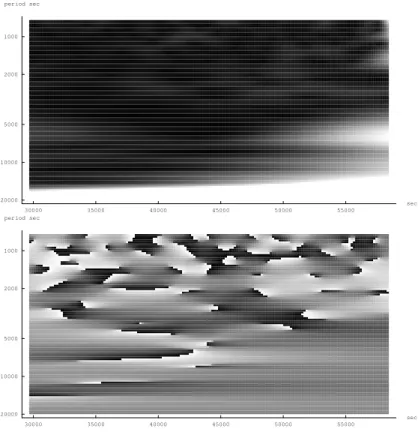
30000 35000 40000 45000 50000 55000 sec 1000 2000 5000 10000 20000 period sec 30000 35000 40000 45000 50000 55000 sec 1000 2000 5000 10000 20000 period sec
Figure 13: Absolute value and phase of Eq. 19 applied to the tick data of British Airways and British Telecom as shown above.
Figure 14: A screen shot from “Algorithmic Echolocation”, an interactive installation by two of the authors (R.Guardans and A.Mathias) and others, shown at the exhibition cycle
Banquete(2003; Palacio de la Virreina, Barcelona; ZKM, Karlsruhe; Medialab, Madrid). The installation allows the visitor to navigate through the Vostok data material (here the CO2
data set) in a way that is inspired by a sound sampler, using loops and variable playback speed. The data is analyzed using Eq.17, and the absolute values are displayed as elevation and the phase as vector field. Further, an animated graphic representation of the equation acting on the data is shown. Beyond graphics, the original data and the spectral analysis result are used to directly control sound parameters of a software synthesizer, a process called audification.
Acknowledgements
We are grateful for stimulating discussions with Kurt Br¨auer, Sebastian Fischer, Frank Schlottmann and Thomas St¨umpert.
References
Bretthorst G (2000). “Nonuniform Sampling: Bandwidth and Aliasing.” In G Erickson (ed.), “Maximum Entropy and Bayesian Methods,” Kluwer.
Chui C (1992). An Introduction to Wavelets. Academic Press, Boston.
Daubechies I (1987). “The Wavelet Transform, Time-Frequency Localization and Signal Anal-ysis.”IEEE Transactions on Information Theory,36, 961–1005.
Holschneider M (1995). Wavelets – An Analysis Tool. Oxford University Press, New York. Lomb N (1976). “Least-Squares Frequency Analysis of Unequally Spaced Data.”Astrophysics
and Space Science,39, 447–462.
Penrose R (1955). “A Generalized Inverse for Matrices.” In “Proceedings of the Cambridge Philosophical Society 51,” pp. 406–413.
Petit JRet al (1999). “Climate and Atmospheric History of the Past 420 000 Years from the Vostok Ice Core, Antarctica.”Nature,399, 429–436.
Press W, Teukolsky S, Vetterling W, Flannery B (1992). Numerical Recipes in C: The Art of Scientific Computing, pp. 575–584. Cambridge University Press, 2 edition.
Scargle J (1976). “Studies in Astronomical Time Series Analysis II. Statistical Aspects of Spectral Analysis of Unevenly Spaced Data.” Astrophysics and Space Science, 302, 757– 763.
Affiliation:
Adolf Mathias
ZKM - Center for Art and Media Institute for Basic Research 76135 Karlsruhe, Germany E-mail: [email protected]
Florian Grond
ZKM - Center for Art and Media Institute for Basic Research 76135 Karlsruhe, Germany E-mail: [email protected]
Hans Diebner
ZKM - Center for Art and Media Institute for Basic Research 76135 Karlsruhe, Germany E-mail: [email protected] Detlef Seese University of Karlsruhe (TH) Institute AIFB 76128 Karlsruhe, Germany E-mail: [email protected] Ramon Guardans
Alvarez de Castro 12, Madrid 28010 Medialab Madrid, Madrid 28015 Spain
E-mail: [email protected]
Miguel Canela
University of Barcelona
Department of Applied Mathematics and Analysis Barcelona 08007, Spain
E-Mail: [email protected]
Journal of Statistical Software
Submitted: 2003-07-22May 2004, Volume 11, Issue 2. Accepted: 2004-05-19
![Figure 4: Eq. 3 applied to sin 39t + sin(39 + 2π)t randomly sampled over [0, 1] with increasing density (100, 400, 2000 and 10000 points, curve plot density increasing with sample density).](https://thumb-us.123doks.com/thumbv2/123dok_us/35418.2504990/6.892.199.713.158.487/figure-applied-randomly-sampled-increasing-density-density-increasing.webp)