Title
Leverage, Volatility and Executive Stock Options
Author(s)
Choe, Chongwoo
Citation
Issue Date
2001-12
Type
Technical Report
Text Version
publisher
URL
http://hdl.handle.net/10086/13851
Discussion Paper Series A No.420
Leverage, Volatility and Executive Stock Options Leverage, Volatility and Executive Stock OptionsLeverage, Volatility and Executive Stock Options Leverage, Volatility and Executive Stock Options
Chongwoo Choe
(Australian Graduate School of Management, University of New South Wales and
University of Sydney, Australia/
The Institute of Economic Research, Hitotsubashi University)
December 2001
The Institute of Economic Research Hitotsubashi University
Leverage, Volatility and Executive Stock Options
∗Chongwoo Choe
Australian Graduate School of Management
University of New South Wales and University of Sydney
Please send all correspondence to: Chongwoo Choe
Australian Graduate School of Management University of New South Wales
Sydney, NSW 2052 AUSTRALIA
(Phone) +61 2 9931 9528 (Fax) +61 2 9313 7279 (Email) [email protected]
∗ This paper was first written during my visit to the Bank of Portugal and the University of Bristol. I am grateful to Bernardino Ad˜ao, Isabel Correia, Gerry Garvey, Ian Jewitt, In-Uck Park, Pedro Teles, semi-nar participants at the Australian Graduate School of Management, La Trobe University, Monash University, and the University of Sydney for stimulating discussions, and to the Bank of Portugal for financial support. The current paper is a considerable revision of an earlier paper titled “Executive Stock Options and Invest-ment Choice”, which has benefited from many constructive comInvest-ments from an anonymous referee. The usual disclaimer applies.
Leverage, Volatility and Executive Stock Options
Abstract
This paper studies how an optimal wage contract can be implemented using stock options, and derives the properties of the optimal contract with stock options. Specifically, we show how the exercise price and the size of the option grant should change in respose to changes in exogenous parameter. First, for a fixed exercise price of executive stock options, the size of the option grant decreases in the riskiness of a desired investment policy, decreases in the volatility of return from the risky project, and increases in leverage. Second, for a fixed size of the option grant, the optimal exercise price of managerial stock options increases in the riskiness of a desired investment policy, increases in the volatility of return from the risky project, and decreases in leverage. Several empirical predictions are drawn from these conclusions regarding the pay-performance sensitivity of management compensation.
KEY WORDS: Leverage, volatility, executive stock options, optimal contract. JEL CLASSIFICATION: D82, G32, J33.
1. Introduction
The last decade has seen an explosive use of stock options as an incentive device for top management of corporations. For example, Yermack (1995) estimates that, for 793 major US corporations, the value of stock options represented about one-third of total CEO compensation in the early 1990s. Murphy (1999) reports that the value of executive stock options has increased to more than a half of total compensation in 1998 for top 200 US corporations. Despite the recent global downturn, stock options are still one of the most important tools for corporations around the world in motivating their chief executives officers.
Since the seminal work of Jensen and Murphy (1990), there is now a large body of empirical literature studying the incentive effects of executive stock options.(1) These studies generally report that the most of incentives to CEOs are provided through stock options and that, when options are properly valued, the pay-performance sensitivity of executive compensation is larger than that originally estimated by Jensen and Murphy (1990). Though not as rich as the empirical literature, several theoretical studies focus on how stock options motivate managers. Haugen and Senbet (1981) show that the mix of put and call options can mitigate the asset substitution problem. Carpenter (2000) argues that executive stock options may not necessarily encourage excessive risk-taking for risk-averse portfolio managers. However, her focus is on the manager’s trading strategy, rather than on the characterization of an optimal contract with stock options. Hall and Murphy (2000) present an example where executive stock options granted at-the-money can be optimal. Saly (1994) argues that repricing executive stock options can be optimal in business downturn. Acharya et al. (2000) also show that resetting the exercise price of executive stock options can be optimal under some circumstances. The positive effect of repricing is generally supported by Brenner et al. (2000), and Chance et al. (2000).
The purpose of this study is to provide additional insight to the theoretical literature by characterizing an optimal contract with stock options. In doing so, we extend the model of John and John (1993), in which the manager can gather private information before making an
(1) Some examples are Yermack (1995), Core and Guay (1998), Hall and Liebman (1998), and Aggarwal and
investment decision, and the owner’s equity and external debt are necessary for the investment. The manager’s investment decision is a dichotomous one of choosing between a safe and a risky project. The owner designs a managerial contract which can induce the manager to implement the investment policy desired by the owner. The managerial contract consists of a base salary and incentive components. Incentive components are either a bonus based on the return from investment or stock options. Managerial contracts as well as the manager’s investment decision are observed by the market, which then prices the firm and the debt in a way consistent with these observations.
This paper first shows how a conventional wage contract should be designed in an incentive-compatible way. This involves rewarding the manager with a bonus when the risky project with a positive net present value is chosen. The resulting optimal contract thus has the usual monotonicity property. We then show how stock options can replicate the incentives provided through the wage contract. This enables us to better understand the nature of incentives that stock options generate. Specifically, we demonstrate how the bonus parameter under the wage contract is related to the exercise price and the size of the option grant under the stock options contract. Next we perform the comparative statics of the optimal stock options contract with respect to the firm’s leverage and the volatility of return. This generates a number of testable hypotheses.
First, for a fixed exercise price of managerial stock options, the size of the option grant decreases in the riskiness of a desired investment policy, decreases in the volatility of return from the risky project, and increases in leverage. The intuition behind the first result becomes clear if one identifies the value of stock options with the bonus under the wage contract. For a fixed exercise price, the value of options increases when the size of the option grant increases. Since the bonus is a reward when the manager takes a profitable risk, it follows that the size of the option grant should decrease if the owner wants to induce the manager to choose a more conservative investment policy. Next, an increase in the volatility of return increases the value of options, which would lead the manager to choose the risky project more often unless such incentives are countered. Thus, for a fixed exercise price, the size of the option grant needs to be decreased when the volatility increases. The size of the option grant in our model reflects the pay-performance sensitivity of executive compensation. It follows then that the
pay-performance sensitivity should decrease in the volatility of the firm’s return.(2) Finally, an increase in leverage decreases the value of options by raising the effective exercise price of options, which is the sum of the exercise price and the face value of debt. For a fixed exercise price, the size of the options grant should therefore increase when the firm has more debt in its capital structure. This leads to a hypothesis that the pay-performance sensitivity should increase in leverage.(3)
Second, for a fixed size of the option grant, the optimal exercise price of managerial stock options increases in the riskiness of a desired investment policy, increases in the volatility of return from the risky project, and decreases in leverage. This follows straightforwardly since the exercise price and the size of the option grant are inversely related in determining the value of a stock options contract. While the exercise price of executive stock options is also a contractual variable, it is usually the case that the exercise price is set equal to the grant date stock price. It warrants an explanation whether such a practice of granting at-the-money options is the result of optimal contracting or out of mere convenience.(4) Our result shows how the exercise price has to be chosen optimally when exogenous parameters change. In particular, the last observation suggests that higher leverage calls for a decrease in the exercise price to leave the effective exercise price unchanged. This prediction is supported by Garvey and Mawani (1999) who find from Canadian data that more levered firms tend to set the exercise price lower so that the effective exercise price faced by executives remains more or less independent of leverage.
An additional conclusion from this study is that financial leverage should not necessarily distort the investment decision made by managers who are motivated by self-interest. Nu-merous previous studies have provided various solutions to this asset substitution problem.
(2) Using the data from the 1,500 S&P corporations for the period of 1993-1996, Aggarwal and Samwick
(1999) report that the executive’s pay-performance sensitivity decreases in the variance of the firm’s perfor-mance. They provide an alternative explanation based on the risk-sharing aspect of an optimal contract for risk-averse executives.
(3) John and John (1993) analyzed optimal CEO compensation that mitigates the asset substitution problem
when the firm has debt in its capital structure. While their focus is not on executive stock options per se, they derive a conclusion that more levered firms should sever the link between managerial interests and shareholder interests by making smaller the pay-performance sensitivity parameter of the managerial contract. The difference between their result and ours is explained in detail in section 3.
(4) Hall and Murphy (2000) present an example with risk-averse managers in which the firm’s cost
mini-mization problem leads to a range of optimal exercise prices which includes the grant date stock price. But it is not a definitive answer to why almost all options are granted at the money.
Zender (1991), and Aghion and Bolton (1992) show how a firm’s internal control should be optimally allocated in a state-contingent way to different security-holders. Dewatripont and Tirole (1994) extend the analysis to argue how such a mechanism can indeed control man-agerial moral hazard. Berkovitch and Israel (1996), and Berkovitch et al. (1999) show how a firm’s capital structure can discipline managers through the optimal replacement policy of managers by claim-holders. While an optimal capital structure is not an issue in this study, this paper is also concerned with optimal managerial incentives in the presence of external debt. In particular we show how the exercise price of managerial stock options should be adjusted to make contracts incentive compatible when the firm has debt in its capital structure.
The rest of the paper is organized as follows. The next section presents the model. Section 3 solves the model for an optimal contract based on verifiable return. Section 4 analyzes optimal contracts with stock options and provides the main comparative static predictions of the model. The final section summarizes the main findings and concludes. Proofs not provided in the main text are relegated to the appendix.
2. The Model
Our basic model is a slightly modified version of John and John (1993). The firm consists of two agents: the owner (or the representative shareholder) and the manager. There are two investment projects. A safe project, denoted S, returns I > 0 for sure. A risky project, denoted R, returns x with probability q and 0 with probability 1−q. To make the results of the paper in line with those from traditional option pricing models, we introduce additional randomness to John and John’s model by assuming that x is lognormally distributed with
ln x∼n(µ, σ2). Denote the mean of x by π ≡exp(µ+12σ2). The distribution function and the density function of x are denoted by G(x) and g(x), respectively. To undertake either project, the owner needs to issue debt for partial finance. The debt is a zero-coupon bond, repayable at the terminal date, whose face value is denoted by D. The net interest rate is assumed to be zero, and the manager’s reservation utility is denoted by W >0. Both agents are assumed to be risk neutral, interested only in maximizing expected payoffs. Assuming risk neutrality allows us to separate the risk-sharing aspect from the incentive aspect of optimal
contracts. Since our focus is on the qualitative characteristics of an optimal contract rather than the quantitative valuation of executive stock options, risk aversion is not likely to bring about changes to the main results of the paper.
Before making a project choice decision, the manager alone can gather information, which, for simplicity, is identified with the observation of q. Without information gathering, the owner and the manager share the common belief about the distribution of q which has a positive, differentiable density function f(q), and a distribution function F(q). Given the observation of q, the expected return from the risky project is R0∞qx dG(x) = qπ where
π =R∞
0 x dG(x) = exp(µ+ 1 2σ
2) was defined earlier as the mean of x. Consider now an
investment policy which selects R for all q0∈[q,1] and S otherwise. This investment policy will be simply denoted by q, a cutoff probability above which the risky project is chosen. Then the expected return from the investment policy q is
V0(q)≡ Z q 0 I dF(r) + Z ∞ 0 Z 1 q rx dF(r) dG(x)≡F(q)I+β(q)π (1) where β(q) ≡ R1
q rdF(r) is the ex ante probability of π given the investment policy q.
Since both agents are risk neutral, the first-best investment policy is the one that maximizes
V0(q). It is easy to see that the first best investment policy is q∗ = πI. That is, q∗ is
a cutoff probability above which the risky project has a larger expected return than the safe project.
Since the manager is risk neutral, it is not hard to imagine that the owner can implement the first best investment policy using a variety of incentive contracts. However, whether the first best investment policy is in the interest of the owner depends on the cost of implementing such a policy. This is particularly relevant if the managerial contract has to observe limited liability. In the remainder of the paper, we study two types of such contracts: conventional wage contracts with a return-based bonus and stock options contracts where the bonus is replaced by gains from option exercise.
The timing of the model is as follows. Initially, the owner offers the manager a contract and issues debt. When pricing the debt, the market observes the managerial contract and correctly infers the investment policy that is implied by the contract. Next, the manager observes q,
and chooses an investment project. At the terminal date, the return from the chosen project is realized and the terms of initial contract are executed including the repayment of debt. To simplify matters, we assume that debt is senior to any cash compensation to the manager. Otherwise, the default probability of debt will depend on the manager’s wages, which will in turn affect the price of debt. The only source of private information in the model is the manager’s observation of q. All other aspects of the model are publicly observable. When they are also verifiable, hence contractible, our focus will be on return-based contracts. When we discuss contracts with stock options, we will simply assume that returns are not verifiable. Nonetheless, they are publicly observable, and will be incorporated in the value of the firm.
3. Optimal Return-Based Contracts
Since the manager is risk neutral and makes a discrete choice of R or S, one can consider a variety of monotonic contracts that are incentive compatible. In this section we focus on linear contracts given by (a, B)≥0 such that the manager receives B if S is chosen, and
ay if R is chosen and the return less debt repayment is y. Thus when the manager chooses
R, her compensation is 0 with probability 1−q and a(x−D)+ ≡ max{a(x−D), 0}
with probability q. Such contracts satisfy limited liability since both a and B are nonnegative. We further restrict attention to contracts satisfying individual rationality and incentive compatibility for the manager.(5) Before these constraints are explicitly stated, it is convenient to simplify the investment policy that will be chosen by the manager. For any contracts satisfying limited liability, the manager’s investment policy can be represented by a cutoff rule. Suppose the manager chose R given the observation of q0. Then for any q > q0, the manager should again choose R as the expected utility is q(ay) ≥q0(ay). Therefore, the investment policy includes the interval [q0,1] at which R is chosen. The implication is that, given any contract, the manager follows a cutoff rule for project choice.
To find the expressions for the expected utilities of the manager and the owner, let us first see how debt will be priced in a rational market. It was assumed earlier that the market
(5) It is a routine to check that the revelation principle holds in the present model so that restricting attention
observes the managerial contract and infers the investment policy correctly as implied by the incentive compatibility constraint. With further assumptions that debt is senior to the manager’s compensation, and that debt can be repaid with probability one if the safe project is chosen, i.e., D+B ≤I, the price of debt is the expected payment at the terminal date. Thus, if the market expects the investment policy q, then the price of debt is given byRq
0 D dF(r) + R1 q h RD 0 rx dG(x) + R∞ D rD dG(x) i
dF(r). Here, the first part of the second integrand reflects the residual claimancy of debt when the return is less than D. Since x is lognormally distributed with ln x∼n(µ, σ2), we have R0Dx dG(x) =exp(µ+12σ2)N
ln D−µ−σ2 σ and R∞ D D dG(x) =DN µ−ln D σ
where N is the cumulative standard normal density function. Using π =exp(µ+12σ2), the price of debt can be determined in pretty much the same way
as in the risk neutral valuation of contingent claims (e.g., Brennan, 1979).
Lemma 1: If the market expects the investment policy q, then the price of debt with face value D is given by F(q)D+β(q)H(D) where H(D) ≡ πN
ln D−ln π σ − 1 2σ + DN ln π−ln D σ − 1 2σ
is the expected repayment of debt under the risky project.
Given the contract (a, B), the manager can secure the base salary (B) by choosing the safe project, and the share (a) of return after debt repayment by choosing the risky project. Thus the manager’s expected utility given the investment policy q is
U(q, a, B) ≡ Z q 0 B dF(r) + Z ∞ D Z 1 q ra(x−D) dG(x)dF(r) =F(q)B+β(q)a[π−H(D)]. (2)
We now turn to the owner’s expected utility. Given the way debt is priced rationally, the owner receives the price of debt initially, which cancels exactly with the expected repayment of debt at the terminal date. Therefore debt does not appear in the owner’s problem. This becomes evident once we write the owner’s expected utility given the investment policy q and the managerial contract (a, B):
V(q, a, B)≡F(q)D+β(q)H(D) + Z q 0 (I−B−D) dF(r) + Z 1 q Z ∞ D r(1−a)(x−D) dG(x)dF(r) =F(q)I+β(q)π−nF(q)B+β(q)a[π−H(D)] o =V0(q)−U(q, a, B) (3)
where V0(q) was defined in (1) as the expected return from the investment policy q. In the
first equality of (3), the first two terms are the price of debt, the second term is the owner’s payoff under the safe project, and the last term represents the owner’s share (1−a) of return from the risky project after debt repayment. Note also that U(q, a, B) +V(q, a, B) = V0(q),
hence the expected return is shared between the owner and the manager.
Incentive compatibility can now be stated. If the owner wants the manager to choose the investment policy ˆq, then (a, B) has to be such that the manager’s expected utility from choosing ˆq should not be smaller than those from any other investment policies.
(IC) : ˆq is a unique maximizer of U(q, a, B) =F(q)B+β(q)a[π−H(D)]. (4)
An optimal contract can be found from the owner’s problem:
Maximize(ˆq,a,B) V(ˆq, a, B) s.t. (a, B) ≥0, U(ˆq, a, B)≥W and (IC). (5)
In solving the problem (5), we first simplify (IC) using the relevant first-order condition. Straightforward calculation yields
Lemma 2: (IC) is equivalent to a= qˆ[π−BH(D)] >0.
The implication of Lemma 2 is the usual monotonicity of an optimal contract. That is, at any incentive-compatible contract, the manager’s compensation is larger when the return is higher. With a= qˆ[π−BH(D)], the manager’s expected utility becomes U(ˆq, a, B) =B[F(ˆq) +
reduce B until the individual rationality constraint is binding. Moreover, since the expected return from any investment policy is shared between the owner and the manager, and since the manager’s individual rationality constraint is binding, the owner will always want to implement a policy that maximizes the expected return. But this is the first-best policy given by q∗= πI. The discussions so far lead to
Proposition 1: An optimal return-based contract implements the first-best investment policy q∗ and is given by a= Wq∗F[π(−q∗H)+(Dβ()]q−∗1) and B =
q∗W q∗F(q∗)+β(q∗).
The reason why the first-best investment policy is also in the interest of the owner even in the presence of debt is that the market prices debt rationally. If debt is given exogenously instead of priced optimally, then there is the usual problem of asset substitution. That is, for any given D ≥ 0, the owner would want to implement the asset substitution policy, ˜
q ≡ I−D π−D ≤q
∗. When D is optimally priced at the time of issue, however, such a problem
does not exist.(6)
The optimal contract in Proposition 1 has a natural interpretation. The manager can secure B by choosing the safe project, which can be interpreted as a base salary. The parameter a reflects the sensitivity of the manager’s compensation to the return, which may be called a pay-performance sensitivity parameter. If the manager chooses the risky project, then her compensation can be larger or smaller than the base salary depending on the return from the risky project. In particular, a sufficiently low return from the risky project can result in the manager’s compensation lower than the base salary.(7)
With this interpretation, several observations can be made. First, to induce a more conservative policy (higher q∗), the owner needs to increase the base salary and decrease the pay-performance sensitivity parameter. This is obvious since the bonus or the performance pay is relevant only when the manager takes risks. Second, the increase in the volatility (σ) of return from the risky project should decrease the pay-performance sensitivity parameter. This
(6) We do not mean to say that the asset substitution problem is not important. At any point in time, the
firm may have some level of debt which has been carried over from planning periods long before. Insofar as there is time inconsistency in pricing debt and covenants are not perfect, the asset substitution problem could be real.
(7) Salary reduction for CEOs in financially distressed firms is often observed in practice (Gilson and
is mainly due to the limited liability of the managerial contract. With a larger volatility, the performance pay is larger when the manager takes risks as it increases the option value of the performance pay. To counter this incentive, the pay-performance sensitivity parameter should be set lower. As we will see in the next section, this observation naturally extends to the case when the manager is paid in options.
Finally, the base salary is independent of the level of debt while the pay-performance sensitivity parameter increases as the level of debt increases. The last point is in contrast to John and John (Proposition 5) who show that the pay-to-shareholder-wealth sensitivity parameter decreases in the face value of debt. The difference between the above result and John and John’s stems mainly from the way compensation contracts are structured. In John and John, the base salary is paid regardless of the financial situation of the firm while insolvency incurs an exogenous penalty to the manager. Therefore the only endogenous variable that has the incentive effect is the pay-performance sensitivity parameter. Thus it follows that a higher face value of debt should be accompanied by a smaller pay-performance sensitivity parameter, which has to be compensated through an increase in the base salary to keep the manager’s individual rationality constraint satisfied. In our model, the base salary has an incentive effect as it is paid only when the manager chooses the safe project while the manager’s compensation given the risky project is proportional to the return after debt has been repaid. Since the base salary is independent of the level of debt, and a higher face value of debt means lower return less debt repayment, the pay-performance parameter has to increase in the level of debt to keep the manager’s individual rationality constraint satisfied.(8) These observations are summarized below. Proposition 2: ∂q∂B∗ ≥0, ∂a ∂q∗ ≤0, ∂B ∂D = 0, ∂a ∂D ≥0, ∂B ∂σ = 0, ∂a ∂σ ≤0.
Interestingly, the pay-performance sensitivity parameter decreases in the volatility of re-turn from the risky project only when the firm has debt in its capital structure. Suppose the owner has enough internal capital so that D→0. Then limD→0H(D) = 0, and so ∂σ∂a = 0.
Thus the volatility of return from the risky project does not affect the manager’s performance
(8) Yermack (1995) finds no significant association between financial leverage and incentives from stock
pay in unlevered firms. The reason why this is the case is that, in our model, the manager’s performance pay is dependent on the return from the project after debt has been repaid. In other words, it is a function of the shareholder value, rather than the value of the firm.(9) If the firm has debt in its capital structure, then the volatility affects the shareholder value by changing the default probability of debt, which has to be taken into account when designing managerial contracts. This as well as much of the observations made in this section can be seen in the case when the manager is paid in stock options, to which we now turn.
4. Optimal Contracts with Stock Options
Denote a contract with stock options by Σ ≡ (B, α, k) where B ≥0 is a base salary payable when the safe project is chosen, and α is the fraction of the value of equity which the manager can buy at the terminal date at an exercise price given by k ≥ 0. In other words, α represents the size of call options on stocks awarded to the manager. We assume that the manager can costlessly borrow funds to exercise options(10) and then immediately resell the stocks. Moreover, instantaneous reselling of stocks after the option exercise implies that options merely represent a financial incentive device. The issues of control shift when the manager holds on to stocks after exercising options or how the exercise of options changes the stock price are beyond the scope of this paper.
As before we will solve for an optimal contract by studying the owner’s optimal problem subject to individual rationality and incentive compatibility constraints. Suppose the owner wants the investment policy ˆq ∈(0,1) to be implemented. For a contract Σ≡(B, α, k) to be incentive compatible, the manager who observed q <qˆ should not have incentives to select
R. That is, we must have B+α(I −D−B−k)+ ≥ qαR∞
0 (x−D−k)
+ dG(x) where
the right-hand side of the inequality is due to the fact that the options are worthless with probability 1−q if the risky project is chosen. Similarly, the manager who observed q ≥qˆ
(9) Dewatripont and Tirole (1994) use an incomplete contracting approach and the allocation of control to
explain why the manager’s compensation is linked to the shareholder value.
(10) Since we assume that the risk-free interest rate is zero, the manager can, for example, do this by using
should not have incentives to select S, or B+α(I−D−B−k)+ ≤qαR0∞(x−D−k)+ dG(x). Therefore we have the following incentive compatibility constraint.
Lemma 3: The owner can almost surely implement the investment policy qˆ with a
contract Σ≡(B, α, k) if and only if B =αqˆR0∞(x−D−k)+ dG(x)−(I−D−B−k)+.
The left-hand side of the equality in Lemma 3 is the loss in the base salary from choosing the risky project, which could have been secured by choosing the safe project. The other side of the equality is the net gains from options when the risky project is chosen instead of the safe project at the cutoff probability ˆq. Thus Lemma 3 implies that the loss and the gains have to be balanced at the cutoff probability ˆq. Given this, the manager with q <qˆ will choose the safe project since the loss outweighs the gains. Similarly, the manager with q≥qˆ will choose the risky project.
If Σ = (B, α, k) is incentive compatible for the policy ˆq, then the manager’s expected utility can be expressed as
U(ˆq,Σ)≡ Z qˆ 0 B+α(I −D−B−k)+ dF(q) + Z 1 ˆ q Z ∞ 0 qα(x−D−k)+ dG(x)dF(q) =αF(ˆq)ˆq+β(ˆq) Z ∞ 0 (x−D−k)+ dG(x). (6)
The last integral in (6) is the value of an option on the return from the risky project. Given the assumption that x is lognormally distributed, it can be shown to be equal to the Black-Scholes value of a European option when the exercise price is D+k, and the risk-free interest rate is zero.(11) Denote it by P(D+k). Then we have
Lemma 4: P(D+k) ≡R∞
0 (x−D−k)
+ dG(x) = πN(Z
D+k +σ)−(D+k)N(ZD+k)
where ZD+k ≡ ln π−lnσ(D+k) −12σ.
(11) In reality, the value of options to company executives would be less than the Black-Scholes value for
various reasons. First, company executives are risk averse with limited opportunities to diversify their financial and human capital portfolios. Second, unlike usual stock options, there are many trading restrictions on executive stock options. See, for example, Hall and Murphy (2000). While these factors will become important in quantitative valuation of executive stock options, they are unlikely to change the qualitative prediction of comparative static analyses, which are the main focus of this paper.
As shown above, debt effectively increases the exercise price of options, hence reducing the Black-Scholes value of options. What it suggests is that more levered firms should make necessary adjustments in managerial contracts to take this into account. In the current context, this could be done by either increasing the size of the option grant, or increasing the base salary, or decreasing the exercise price. However, increasing the size of the option grant makes the risky project more attractive, while increasing the base salary will make the safe project more attractive. Thus an incentive-neutral way to account for leverage is to adjust the exercise price since the effective exercise price of options is D+k. As mentioned before, Garvey and Mawani (1999) find that more levered firms tend to set the option exercise price lower so that the effective exercise price remains more or less constant within an industry.
For future reference, we document below how P(D+k) changes as D, k and σ change. As usual, the value of a call option decreases in the exercise price and increases in the volatility of return. Moreover, debt and the exercise price have the same effect on the value of a call option since the effective exercise price is the sum of the two.
Lemma 5: ∂P(∂DD+k) = ∂P(∂kD+k) =−N(ZD+k)≤0, and ∂P(∂σD+k) =πn(ZD+k+σ)≥0
where N(·) is the cumulative standard normal density function and n(·) is the standard normal density function.
If Σ = (B, α, k) is incentive compatible for the policy qˆ, then the owner’s expected utility can be written as
V(ˆq,Σ)≡F(q)D+β(q)H(D) + Z qˆ 0 [I−B−D−α(I−B−D−k)+]dF(q) + Z 1 ˆ q Z ∞ D q(x−D) dG(x)dF(q)− Z 1 ˆ q Z ∞ D qα(x−D−k)+ dG(x)dF(q) =V0(ˆq)−U(ˆq,Σ) (7)
where V0(ˆq) was defined in (1) as the expected return from the investment policy ˆq. Thus
the expected return is again shared between the owner and the manager. Moreover the owner can always choose an incentive-compatible contract which makes the manager’s individual rationality constraint binding. This can be seen from the manager’s expected utility in (6): if
the individual rationality constraint is not binding, then the owner can either decrease α or increase k until the constraint is binding. Therefore, an optimal contract again implements the first-best investment policy as it maximizes the expected return. Combining the incentive compatibility constraint for the first-best investment policy q∗, and the binding individual rationality constraint, we have
Proposition 3: Σ = (B, α, k) is an optimal contract with stock options if and only if
B =α
q∗P(D+k)−(I−D−B−k)+
and α
F(q∗)q∗+β(q∗)
P(D+k) =W.
As is evident from Proposition 3, there is a continuum of optimal contracts since three variables (B, α, k) are to be determined from two equations. For example, if the base salary is fixed for some reasons,(12)then the exercise price and the size of the option grant can be chosen
from the positive relation given by the individual rationality constraint. To study the exact relations between these variables and various exogenous parameters of the model, we conduct comparative static analyses below. In doing so, we need to fix one contractual variable since there are three variables but only two equations on which to base comparative statics.
We will divide the incentive compatibility constraint into two cases depending on the exercise price. Suppose first that the exercise price is set high enough so that options are out of the money when the safe project is chosen, i.e., VS ≡ I−D−B < k where VS is
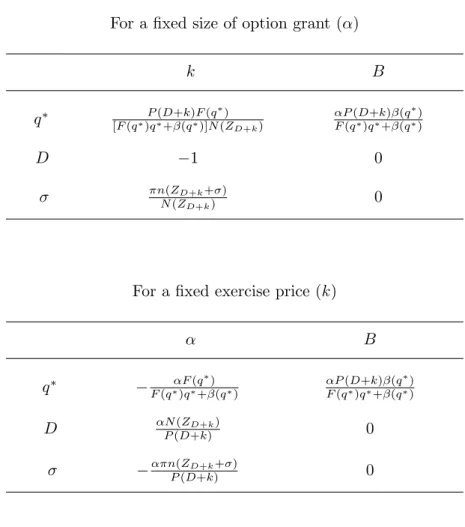
the value of equity when the safe project is chosen. Then the manager is paid entirely in fixed salary when the safe project is chosen, and in options when the risky project is chosen. The incentive compatibility constraint in this case simplifies to B =αq∗P(D+k), and the relation between the exercise price and grant size is determined completely by the individual rationality constraint alone. Since there is a continuum of (exercise price, grant size) satisfying the individual rationality constraint, we need to fix one of these variables for comparative statics purpose. The following proposition summarizes the results of the comparative statics. The exact expressions are provided in Table 1 where the two contractual variables in the first row are differentiated with respect to the three parameters in the first column.(13)
(12) In case of the US, the introduction of ‘the million dollar rule’ has led to the clustering of CEOs’
non-performance related pay around 1 million dollars.
(13) Since the relation between the exercise price and grant size is determined completely by the individual
Proposition 4: Let (B, α, k) be an optimal contract with stock options for which
k > VS. Then for a fixed size of the option grant α, ∂q∂k∗ ≥0, ∂k ∂D ≤0, ∂k ∂σ ≥0, ∂B ∂q∗ ≥0, ∂B ∂D = ∂B
∂σ = 0. And for a fixed exercise price k, ∂α ∂q∗ ≤ 0, ∂α ∂D ≥ 0, ∂α ∂σ ≤ 0, ∂B ∂q∗ ≥ 0, ∂B ∂D = ∂B ∂σ = 0.
— Table 1 goes about here. —
The intuition behind the above propostion is as follows. Consider first changes in q∗. If the owner wants a more conservative policy (higher q∗), then the value of options has to be adjusted downwards. This can be done by either decreasing the size of the option grant or increasing the exercise price. Therefore, if the size of the option grant is fixed, then a more conservative policy can be induced by increasing the exercise price. Similarly, if the exercise price is fixed, then the size of the option grant has to be reduced to induce a more conservative policy. However, such a unilateral adjustment will lead to the violation of the manager’s individual rationality constraint, which is already binding at the optimal contract. Thus a downward adjustment of option value needs to be accompanied by an upward adjustment in the base salary that leaves the individual rationality constraint intact.
Next, an increase in the level of debt reduces the value of options by increasing the effective exercise price. To offset the manager’s incentive to choose the safe project more often, either the size of the option grant needs to be increased or the exercise price needs to be decreased. As such adjustments will leave the value of options unchanged, simultaneous adjustments in the base salary are not necessary. Finally, an increase in the volatility of return from the risky project increases the value of options, which again calls for either a reduction in the size of the option grant or an increase in the exercise price. Again changes in the base salary are not necessary as the value of options will remain unchanged after the adjustment of the grant size or the exercise price.
These results parallel the findings in Propostion 2. With return-based contracts, the optimal pay-performance sensitivity parameter increases in the level of debt, and decreases in
q∗ and the volatility of return from the risky project. With stock options, such adjustments can be done more flexibly as there are two contractual variables available. If the exercise price is fixed, for example, the comparative statics predictions of the size of the option grant are
exactly consistent with those in Propostion 2.
We now turn to the case where the exercise price is low enough so that options are in the money when the safe project is chosen, i.e., VS ≥ k. Then the incentive compatibility
constraint becomes B =αq∗P(D+k)−α(VS −k), which determines the optimal contract
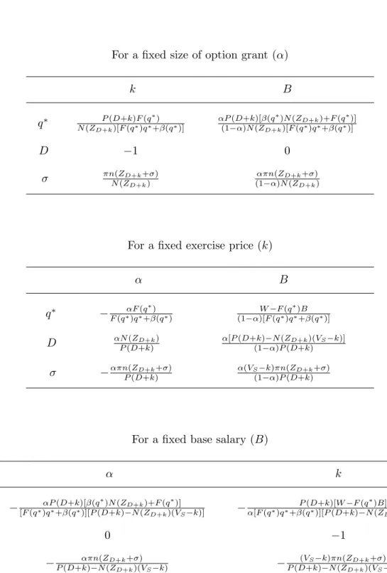
jointly with the individual rationality constraint. Since options affect the manager’s payoff under both projects, comparative static analyses are a bit more complicated. However, the basic intuition is still valid when one notes that the value of options is larger for the manager when the risky project is chosen. The results from comparative statics are summarized below, while the exact expressions are provided in Table 2.
Proposition 5: Let (B, α, k) be an optimal contract with stock options for which
k≤VS. Then for a fixed size of the option grant α, ∂q∂k∗ ≥0, ∂D∂k ≤0, ∂k∂σ ≥0, ∂q∂B∗ ≥0, ∂B
∂D = 0, ∂B
∂σ ≥ 0. For a fixed exercise price k, ∂α ∂q∗ ≤ 0, ∂α ∂D ≥ 0, ∂α ∂σ ≤ 0, ∂B ∂q∗ ≥ 0, ∂B ∂D ≥ 0, ∂B
∂σ ≥0. And for a fixed base salary B, ∂α ∂q∗ ≤0, ∂D∂α = 0, ∂α∂σ ≤ 0, ∂q∂k∗ ≤ 0, ∂k ∂D ≤0, ∂k ∂σ ≤0.
— Table 2 goes about here. —
As mentioned before, the key difference between the two propostions above lies in the way options reward the manager when the safe project is chosen. When the exercise price is low enough, options can be valuable even under very conservative investment policies. However, the benefits of options will be larger if proper risks are taken. This follows since the manager’s compensation under the safe project includes the base salary, which together with the value of options should be balanced with the manager’s compensation under the risky project. This is implied by the incentive compatibility. Therefore, comparative static results of an optimal contract are more or less the same in both cases. Having this in mind, we highlight only the difference bewteen the two propositions.
We start the discussion with the case when the size of the option grant is fixed. Then an increase in the volatility of return from the risky project leads to an increase in the exercise price but not the base salary when the exercise price is high (Propostion 4). However, both the exercise price and the base salary increase in the volatility when the exercise price is low enough (Proposition 5). To understand why this is the case, note that an increase in the exercise price
neutralizes the increase in the value of options under the risky project, which would have resulted from higher volatility. On the other hand, such an increase in the exercise price reduces the value of options under the safe project, which does not depend on the volatility. To satisfy the incentive compatibility constraint, the base salary should be increased to make up for the reduced value of options.
Suppose now that the exercise price is fixed. The base salary does not change in the level of debt nor in the volatility of return when the exercise price is high, but increases in both parameters when the exercise price is low. Consider debt first. A higher level of debt leads to a lower value of options under both projects, which needs to be compensated through an increase in the size of the option grant. But the decrease in option value is larger under the safe project since a dollar increase in debt implies a dollar decrease in the value of equity in this case. Therefore, the base salary needs to be increased to balance the incentives. Next, an increase in the volatility of return increases the value of options only under the risky project. However, a downward adjustment in the size of the option grant reduces the value of options under both projects, which calls for an increase in the base salary.
The final case is when the base salary is fixed. Suppose the owener wants a more conser-vative investment policy (higher q∗). This requires a reduction in the size of the option grant, which will reduce the value of options under both projects, violating the manager’s individual rationality constraint. Thus the exercise price needs to be reduced as well since the base salary cannot be increased. Changes in leverage can be easily accounted for by simply adjusting the exercise price without having to change the size of the option grant. By matching a dollar increase in the level of debt by a dollar decrease in the exercise price, the effective exercise price of options can be held fixed. If the volatility of return from the risky project increases, thereby increasing the value of options under the risky project, then the size of the option grant needs to be decreased to offset the manager’s incentive for excessive risk-taking. However, this will reduce the manager’s compensation under the safe project, which needs to be compensated through a decrease in the exercise price.
The two propositions above lead to a number of hypotheses regardling optimal executive stock options. First, if the firm wants to implement conservative investment policies, then the pay-performance sensitivity reflected in the size of the option grant should unambiguously
decrease and the option exercise price should unambiguously increase. Second, an incentive-neutral way of accounting for leverage is to adjust the option exercise price one-to-one to changes in the level of debt so that the effective exercise price of options remains unchanged. Third, the performance sensitivity does not decrease in the level of debt. Fourth, the pay-performance sensitivity unambiguoulsy decreases in the volatility of the firm’s return. Fifth, an increase in the volatility may increase or decrease the option exercise price depending on how other contractual variables can be flexibly adjusted.
5. Summary and Discussions
This paper has studied how an optimal wage contract can be implemented using stock options, and derived the properties of the optimal contract with stock options. The central thrust of the paper is that the exercise price as well as the size of the option grant should be optimally chosen to motivate managers. The paper has obtained a number of results regarding these contractual variables. First, for a fixed exercise price of executive stock options, the size of the option grant decreases in the riskiness of a desired investment policy, decreases in the volatility of return from the risky project, and increases in leverage. Second, for a fixed size of the option grant, the optimal exercise price of managerial stock options increases in the riskiness of a desired investment policy, increases in the volatility of return from the risky project, and decreases in leverage.
Several empirical predictions can be drawn from these conclusions mainly regarding the pay-performance sensitivity of management compensation when stock options are a primary instrument. First, the pay-performance sensitivity should be higher for firms in growth in-dustries where risk-taking is an essential part of their success. Second, the pay-performance sensitivity should decrease in the volatility of the firm’s stock price. Third, the pay-performance sensitivity should not decrease in the level of debt. And fourth, across firms with a similar pay-performance sensitivity, the option exercise price and the level of debt should be inversely related.
Executive stock options are one of the most widely used tools in motivating top man-agement of corporations. Despite the popularity, our understandind of the instrument is not
entirely satisfactory. At least two directions of further reseach can be suggested. The first con-cerns the near-universal practice of granting options at the money. Hall and Murphy (2000) is an initial attempt to this direction. To understand better the (non)optimality of such a prac-tice, the current model needs to incorporate risk aversion of managers and a richer mechanism whereby the stock price is determined. The second relates to the way different countries treat exercutive stock options differently for the purpose of tax and accounting report.(14) At the core of this question lies the valuation of executive stock options to the firm and to risk-averse executives. By modeling the manager’s preference in a way standard in the option-pricing literature (Brennan, 1979), the current paper could shed some light on this direction.
Appendix
Proof of Proposition 2: We will only show ∂D∂a ≥ 0 and ∂σ∂a ≤ 0. The rest are straightforward. To show ∂D∂a ≥ 0, it suffices to show ∂H∂D(D) ≥ 0 since ∂H∂a(D) ≥ 0. Denote ZD ≡
ln(π D)
σ −
1
2σ and let n(·) be the standard normal density function. Then
∂H(D) ∂D =N(ZD) + ∂ZD ∂D Dn(ZD)−πn(−ZD−σ)
. Using the expression for standard normal density function, it is easy to see that n(ZD)
n(−ZD−σ) =
π
D. Thus Dn(ZD)−πn(−ZD−σ) = 0
implying ∂H∂D(D) =N(ZD)≥0, hence ∂D∂a ≥0. Similarly, ∂H∂σ(D) =−πn(−ZD−σ)≤0,
and so ∂σ∂a ≤0.
Proof of Lemma 3: The incentive compatibility requires B +α(I −D−B −k)+ ≥
qαR0∞(x−D−k)+ dG(x) for all q <qˆ and the reverse inequality for all q ≥ qˆ. Thus
B =α
ˆ
qR∞
0 (x−D−k)
+ dG(x)−(I−D−B−k)+
. Given this, the manager who observed
q <qˆ is strictly better off by choosing S, and the manager who observed q >qˆ is strictly better off by choosing R. Since q has a continuous support so that q = ˆq is an event of measure zero, the claim follows.
Proof of Lemma 4: R∞ 0 (x−D−k) +dG(x) =R∞ D+kx dG(x)−(D+k) R∞ D+k dG(x). Since
x is lognormally distributed with ln x ∼ n(µ, σ) and π ≡ R∞
0 x dG(x) = exp(µ+ 1 2σ
2),
(14) Yermack (1995), and Hall and Liebman (2000) find that the effect of tax and accounting considerations
on the use of executive stock options is not significant in the US, while Klassen and Mawani (1999) report a positive correlation between the two in Canada. This discrepancy may be due to the differences in tax treatment of executive stock options in the two countries.
we have RD∞+kx dG(x) =πN(ZD+k+σ), and R∞ D+k dG(x) =N(ZD+k) where ZD+k ≡ ln π−ln (D+k) σ − 1 2σ. Proof of Lemma 5: ∂P(∂DD+k) = ∂ZD+k ∂D πn(ZD+k +σ)−(D+k)n(ZD+k) −N(ZD+k)
where n(·) is the standard normal density function. Using the expression for standard normal density function, it is easy to show that n(ZD+k+σ)
n(ZD+k) = D+k π . Thus πn(ZD+k + σ)−(D+k)n(ZD+k) = 0 implying ∂P(∂DD+k) = −N(ZD+k) ≤ 0. Similarly, ∂P(∂kD+k) = ∂ZD+k ∂k πn(ZD+k+σ)−(D+k)n(ZD+k) −N(ZD+k) =−N(ZD+k)≤0. Finally, ∂P(D+k) ∂σ = ∂ZD+k ∂s πn(ZD+k+σ)−(D+k)n(ZD+k) +πn(ZD+k+σ) =πn(ZD+k+σ)≥0.
Proof of Proposition 4: The two equations that characterize an optimal contract are
B = αq∗P(D+k) and W = αΨ(q∗)P(D+k) where Ψ(q∗) ≡ F(q∗)q∗ +β(q∗). To simplify notation, we will omit the arguments when necessary. For a fixed value of α, totally differentiating these two equations gives us
αq∗∂P∂k −1 αΨ∂P∂k 0 dk dB = −αP dq∗−αq∗∂D∂PdD−αq∗∂P∂σdσ −αPΨ0dq∗−αΨ∂P∂DdD−αΨ∂P∂σdσ . Thus ∂q∂k∗ = −P(D+k)Ψ0(q∗) Ψ(q∗)∂P ∂k = Ψ(P(qD∗)+Nk()ZF(q∗)
D+k) where the last equality follows from Ψ
0(q∗) =
F(q∗) and ∂P∂k =−N(ZD+k) from Lemma 5. Using Lemma 5 again to note ∂P∂k = ∂P∂D and ∂P
∂σ =πn(ZD+k+σ), the others follow similarly.
If k is fixed, then similar algebra can be applied to the following total differential.
q∗P −1 ΨP 0 dα dB = −αP dq∗−αq∗∂P∂DdD−αq∗∂P∂σdσ −αPΨ0dq∗−αΨ∂D∂PdD−αΨ∂P∂σdσ .
Proof of Proposition 5: The two equations that characterize an optimal contract are
B =αq∗P(D+k)−α(VS−k) and W =αΨ(q∗)P(D+k) where Ψ(q∗)≡F(q∗)q∗+β(q∗),
to which the same algebra used to prove Propostion 4 can be applied. To check the signs of derivatives, note that P(D+k) −N(ZD+k)(VS −k) ≥ 0. This follows since B =
αq∗P(D+k)−α(VS−k)≥0 due to limited liability, which implies P(D+k)≥ VSq∗−k ≥VS−k,
References
Acharya, V. V., John, K. and R. K. Sundaram (2000), “On the Optimality of Resetting Executive Stock Options”, Journal of Financial Economics, 57, 65-101.
Aggarwal, R. and A. A. Samwick (1999), “The Other Side of the Tradeoff: The Impact of Risk on Executive Compensation”,Journal of Political Economy 107, No. 1, 65-105. Aghion, P. and P. Bolton (1992), “An Incomplete Contracts Approach to Financial
Contract-ing”,Review of Economic Studies 59, 473-494.
Berkovitch, E. and R. Israel (1996), “The Design of Control and Capital Structure”, Review of Financial Studies 9, No. 1, 209-240.
Berkovitch, E., Israel, R. and Y. Spiegel (1999), “Managerial Compensation and Capital Struc-ture”,mimeo., Tel Aviv University.
Brennan, M. J. (1979), “The Pricing of Contigent Claims in Discrete Time Models”, Journal of Finance 34, No. 1, 53-68.
Brenner, M., Sundaram, R. K. and D. Yermack (2000), “Altering the Terms of Executive Stock Options”, Journal of Financial Economics 57, 103-128.
Carpenter, J. (2000), “Does Option Compensation Increase Managerial Risk Appetite”, Jour-nal of Finance 55, No. 5, 2311-2331.
Chance, D. M., Kumar, R. and R. B. Todd (2000), “The ‘Repricing’ of Executive Stock Options”, Journal of Financial Economics 57, 129-154.
Core, J. and W. Guay (1998), “Estimating the Incentive Effects of Executive Stock Option Portfolios”, mimeo., Wharton School, University of Pennsylvania.
Dewatripont, M. and J. Tirole (1994), “A Theory of Debt and Equity: Diversity of Securities and Manager-Shareholder Congruence”, Quarterly Journal of Economics 439, 1027-1054.
Garvey, G. T. and A. Mawani (1999), “ Executive Stock Options as Home-Made Leverage: Why Financial Structure Does Not Affect Risk-Taking Incentives”, mimeo., University of British Columbia.
Gilson, S. and M. Vetsuypens (1993), “CEO Compensation in Financially Distressed Firms: An Empirical Analysis”,Journal of Finance 48, No. 2, 425-458.
Hall, B. J. and J. B. Liebman (2000), “The Taxation of Executive Compensation”, NBER Working Paper 7596.
Hall, B. J. and J. B. Liebman (1998), “Are CEOs Really Paid Like Bureaucrats?”, Quarterly Journal of Economics113, No. 3, 653-691.
Hall, B. J. and K. J. Murphy (2000), “Optimal Exercise Prices for Executive Stock Options”,
American Economic Review,Papers and Proceedings 90, No. 2, 209-214.
Haugen, R. A. and L. W. Senbet (1981), “Resolving the Agency Problems of External Capital through Options”,Journal of Finance 36, No. 3, 629-647.
Jensen, M. and K. Murphy (1990), “Performance and Top Management Incentives”, Journal of Political Economy98, No. 2, 225-264.
John, T. A. and K. John (1993), “Top-Management Compensation and Capital Structure”,
Journal of Finance 48, 949-974.
Klassen, K. and A. Mawani (1999), “The Impact of Financial and Tax Reporting Incentives on Option Grants to Canadian CEOs”,mimeo., University of British Columbia. Murphy, K. J. (1999), “Executive Compensation”, in Ashenfelter, O. and D. Card (eds.),
Handbook of Labor Economics, Vol. 3B, Amsterdam: North-Holland, 2485-2563. Saly, P. J. (1994), “Repricing Executive Stock Options in a Down Market”, Journal of
Ac-counting and Economics 18, 325-356.
Yermack, D. (1995), “Do Corporations Award CEO Stock Options Effectively?” Journal of Financial Economics 39, 237-269.
Table 1: Comparative Statics of Optimal Contract
for a High Exercise Price
For a fixed size of option grant (α)
k B q∗ [F(q∗)Pq∗(D+β+(kq)∗F)](Nq∗()ZD+k) αP(D+k)β(q∗) F(q∗)q∗+β(q∗) D −1 0 σ πn(ZD+k+σ) N(ZD+k) 0
For a fixed exercise price (k)
α B q∗ −F(q∗αF)q∗(q+∗β)(q∗) αP(D+k)β(q∗) F(q∗)q∗+β(q∗) D αN(ZD+k) P(D+k) 0 σ −απn(ZD+k+σ) P(D+k) 0
Table 2: Comparative Statics of Optimal Contract
for a Low Exercise Price
For a fixed size of option grant (α)
k B q∗ N(Z P(D+k)F(q∗) D+k)[F(q∗)q∗+β(q∗)] αP(D+k)[β(q∗)N(ZD+k)+F(q∗)] (1−α)N(ZD+k)[F(q∗)q∗+β(q∗)] D −1 0 σ πn(ZD+k+σ) N(ZD+k) απn(ZD+k+σ) (1−α)N(ZD+k)
For a fixed exercise price (k)
α B q∗ −F(q∗αF)q∗(q+∗β)(q∗) W−F(q∗)B (1−α)[F(q∗)q∗+β(q∗)] D αN(ZD+k) P(D+k) α[P(D+k)−N(ZD+k)(VS−k)] (1−α)P(D+k) σ −απn(ZD+k+σ) P(D+k) α(VS−k)πn(ZD+k+σ) (1−α)P(D+k)
For a fixed base salary (B)
α k q∗ − αP(D+k)[β(q∗)N(ZD+k)+F(q∗)] [F(q∗)q∗+β(q∗)][P(D+k)−N(ZD+k)(VS−k)] − P(D+k)[W−F(q∗)B] α[F(q∗)q∗+β(q∗)][P(D+k)−N(ZD+k)(VS−k)] D 0 −1 σ − απn(ZD+k+σ) P(D+k)−N(ZD+k)(VS−k) − (VS−k)πn(ZD+k+σ) P(D+k)−N(ZD+k)(VS−k)