A University of Sussex
PhD
thesis
Available
online
via
Sussex
Research
Online:
http://sro.sussex.ac.uk/
This
thesis
is
protected
by
copyright
which
belongs
to
the
author.
This
thesis
cannot
be
reproduced
or
quoted
extensively
from
without
first
obtaining
permission
in
writing
from
the
Author
The
content
must
not
be
changed
in
any
way
or
sold
commercially
in
any
format
or
medium
without
the
formal
permission
of
the
Author
When
referring
to
this
work,
full
bibliographic
details
including
the
author,
title,
awarding
institution
and
date
of
the
thesis
must
be
given
Quantification Under
Class-Conditional Dataset Shift
David James Frederick Spence
A thesis presented for the degree of
Doctor of Philosophy
• This thesis, in full or in part, has not been previously submitted to this or any other university for a degree.
• None of the material in this thesis has already been submitted as part of required
coursework at any university.
• No part of the thesis results from joint work with other persons other than the
development of the 4dSDA dataset as set out in Section 3.4.1.
David James Frederick Spence
Abstract
Classification is the estimation of the class of each instance in a dataset,quantification is
the estimation of thenumber of instances of each class in a dataset. Quantification
meth-ods typically assume that the data which is being quantified has the same class-conditional distribution as the data on which the quantifier was trained. This thesis addresses the situation where this assumption cannot be made, where there is class-conditional dataset shift between the training data and the test data. The work was motivated by sentiment analysis tasks using tweets on Twitter. By selecting users based on the content of their tweet, the users cannot be considered to have been randomly drawn from the population. In this thesis, domain adaptation methods from classification have been applied to the problem of quantification. Separating the data into explicit sub-domains and quantifying each sub-domain separately can increase quantification accuracy but under certain condi-tions it can also decrease it. An expression for expected quantification error was derived in closed-form with some simplifying assumptions. In tests on real datasets, a method based on this approach gave a modest improvement to quantification accuracy. Constructing a new feature representation has proved successful for domain adaptation in classification. An approach using Stacked Denoising Autoencoders to generate a new feature represen-tation gave a 3.3% relative improvement in quantification accuracy. Finally, a method based on using Kernel Mean Matching for weighting instances in the training set gave a relative improvement in quantification accuracy of 10.7%. Experiments were conducted on publicly available datasets and also on a custom dataset of Twitter users.
I would like to thank...
David Weir and Novi Quadrianto for supervising me. Luc Berthouze for chairing my thesis committee.
My fellow members of the department, in particular Chris Inskip, Oliver Thomas, Matti Lyra and Miro Batchkarov for helping me get things to work.
My friends Ian Handel and Mark Bronsvoort at Edinburgh University and Neil Hawkins at Glasgow University for their general advice on doing a PhD and their specific advice, particularly on statistics.
Thomas Kober for gender labelling the 4dSDA dataset. Chris Inskip for the use of the SDA dataset.
CASM Consulting LLP for the use of Method52. Katie Barnett for putting up with me.
Contents
List of Figures vi
List of Tables xi
List of Variables xiv
1 Introduction 1
2 Literature review 7
2.1 Quantification . . . 7
2.1.1 Classify and count . . . 8
2.1.2 Classify and adjust methods . . . 8
2.1.3 Distribution matching . . . 11
2.1.4 Direct quantification . . . 12
2.1.5 Quantification loss functions . . . 15
2.1.6 Quantification test methods . . . 15
2.1.7 Quantification applied to specific areas . . . 16
2.2 Dataset shift . . . 17
2.2.1 Causality and dataset shift . . . 18
2.2.2 Causes of dataset shift . . . 18
2.2.3 Measures of dataset shift . . . 19
2.3 Unsupervised domain adaptation . . . 22
2.3.1 Mixtures of sub-domains . . . 22
2.3.2 Importance weighting of instances . . . 24
2.3.3 Feature representations . . . 28
2.3.4 Weakly supervised . . . 32
2.4 Quantification under class-conditional dataset shift . . . 32
3 Domain adaptation with explicit sub-domains 34 3.1 Definitions . . . 36 3.1.1 Validation data . . . 37 3.1.2 Test data . . . 38 3.1.3 Extension to sub-domains . . . 38 3.1.4 R* . . . 39
3.1.5 Quantification performance measures . . . 39
3.2 Quantification by matrix-inversion . . . 40
3.3 Quantification with and without sub-domains . . . 41
3.3.1 Method . . . 41 3.4 Initial experiment . . . 45 3.4.1 Dataset . . . 45 3.4.2 Method . . . 47 3.4.3 Results . . . 49 3.4.4 Discussion . . . 53 3.5 Analytic exploration . . . 53 3.5.1 Classes . . . 54 3.5.2 Random variables . . . 54
3.5.3 General closed-form solution . . . 55
3.5.4 Simplification: ntis large . . . 56
3.5.5 Simplification: nv is large . . . 57
3.6 Numerical validation of the closed-form solution . . . 65
3.6.1 Method . . . 65
3.6.2 Results . . . 66
3.7 Quantification accuracy and classifier accuracy . . . 67
3.8 Exploration of explicit sub-domains through simulation . . . 69
3.8.1 Method . . . 69
3.8.2 Simulation settings . . . 70
3.8.3 Validation set sizenv . . . 71
3.8.4 Multiple regression analysis . . . 74
3.8.5 Main-class recall . . . 76
3.8.6 Sub-domain recall . . . 76
3.8.7 Test set size . . . 77
iii
4 Domain adaptation with thresholded sub-domains 79
4.1 Experiment 1: Simulation . . . 80
4.1.1 Method . . . 80
4.1.2 Simulation settings . . . 82
4.1.3 Results . . . 82
4.1.4 Discussion . . . 86
4.2 Experiment 2: UCI datasets . . . 86
4.2.1 Datasets . . . 86 4.2.2 Generation of results . . . 88 4.2.3 Algorithm . . . 89 4.2.4 Parameters . . . 90 4.2.5 Classifier performance . . . 91 4.2.6 Results . . . 91 4.2.7 Discussion . . . 95
4.3 Experiment 3: determining thresholds . . . 96
4.3.1 Single criteria . . . 96
4.3.2 Multiple criteria . . . 97
4.3.3 Evaluation against the held-out UCI test datasets . . . 98
4.3.4 Discussion . . . 101
4.4 Experiment 4: Twitter dataset . . . 101
4.4.1 Twitter Age Friends (TAF) dataset . . . 102
4.4.2 Dataset initial analysis . . . 104
4.4.3 Method . . . 105
4.4.4 Results . . . 105
4.4.5 Discussion . . . 107
4.5 Conclusions . . . 108
5 Domain adaptation by instance weighting 109 5.1 Measuring dataset shift . . . 110
5.2 Datasets . . . 111
5.3 Instance weighting . . . 112
5.4 Kernel Mean Matching (KMM) . . . 113
5.5 Unconstrained Least Squares Importance Fitting (uLSIF) . . . 114
5.6 Instance weights by class . . . 116
5.6.2 Results . . . 120
5.6.3 Discussion . . . 122
5.7 Quantification by instance-weighted classify and adjust (IWCA) . . . 123
5.7.1 Method . . . 124
5.7.2 Results . . . 126
5.7.3 Discussion . . . 133
5.8 Classifier-based sample selection bias correction (SSBC) . . . 134
5.8.1 Method . . . 134
5.8.2 Results . . . 135
5.8.3 Discussion . . . 136
5.9 Iterative test-train bias reduction (ITTBR) . . . 136
5.9.1 Method . . . 138
5.9.2 Algorithm . . . 140
5.9.3 Results . . . 141
5.9.4 Discussion . . . 144
5.10 Conclusions . . . 144
6 Domain adaptation with feature representations 146 6.1 Marginalised Stacked Denoising Autoencoders (mSDA) . . . 147
6.2 Method . . . 148
6.2.1 Code . . . 148
6.2.2 mSDA training time . . . 148
6.2.3 Noise . . . 149
6.2.4 Oversampling from the Target domain . . . 149
6.2.5 Layers . . . 150
6.2.6 Classifier parameters . . . 151
6.2.7 Dataset samples and methods . . . 151
6.3 Results . . . 151
6.3.1 Layers . . . 152
6.3.2 Noise . . . 154
6.3.3 Oversampling from the Target domain . . . 154
6.3.4 Training and test set size . . . 155
6.3.5 Recall . . . 156
6.3.6 By level of bias and by dataset . . . 158
v
6.4 Conclusions . . . 161
7 Conclusions and further work 163 7.1 Datasets and bias . . . 165
7.2 Explicit subdomains . . . 166
7.3 Importance weighting . . . 168
7.4 Feature representation . . . 170
7.5 Direct quantification with biased training sets . . . 171
7.6 Implementation . . . 172
7.7 Last words... . . 172
8 Bibliography 173 A Quantification methods 185 A.1 Forman’sAdjusted Count as matrix-inversion . . . 185
A.2 Saerens et al. [97] probabilistic expectation-maximisation method . . . 186
A.3 Joachims [72] SVM for multivariate performance measures . . . 188
A.4 Hofer [62] distribution matching with Gaussian mixtures . . . 189
B Importance weighting methods 192 B.1 Importance weighting methods generally . . . 192
B.2 Kernel mean matching . . . 193
1.1 Estimated and actual class distribution with theclassify and count method 2
1.2 Estimated vs. actual class proportions using both the classify and count
and theclassify and adjust methods. UCI dev datasets. Data from Section
5.9 . . . 3
1.3 Absolute quantification error using classify and adjust method vs.
class-conditional dataset shift. Data from Section 5.9. 95% confidence intervals. . 4
1.4 Common approach to quantification under class-conditional dataset shift . . 5
3.1 Process for computation of quantification error with and without the use of
sub-domains. See Table 3.2 for key to symbols. . . 42
3.2 Validation of the 4dSDA dataset between datasets . . . 46
3.3 Distribution by estimated year of birth in the 4dSDA dataset . . . 47
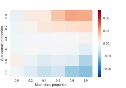
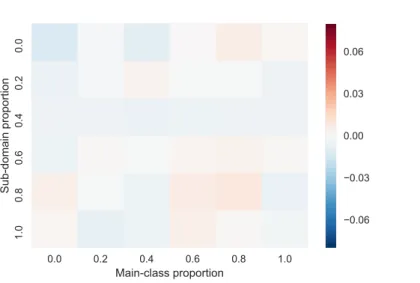
3.4 Mean main-class proportion error vs. main-class proportion and sub-domain
proportion. Classify and count method. 4dSDA dataset . . . 49
3.5 Mean main-class proportion error vs. main-class proportion and sub-domain
proportion. nsd-method. 4dSDA dataset . . . 50
3.6 Mean main-class proportion error vs. main-class proportion and sub-domain
proportion. sd-method. 4dSDA dataset . . . 51
3.7 Mean value of class proportion estimate error . . . 52
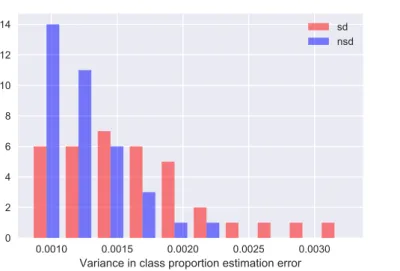
3.8 Variance in class proportion estimate error . . . 52
3.9 Normalised RMSE of estimate for size of main-class α: simulation values
less values from Equations 3.97 and 3.112 vs. log10 of size of validation set nv . . . 67
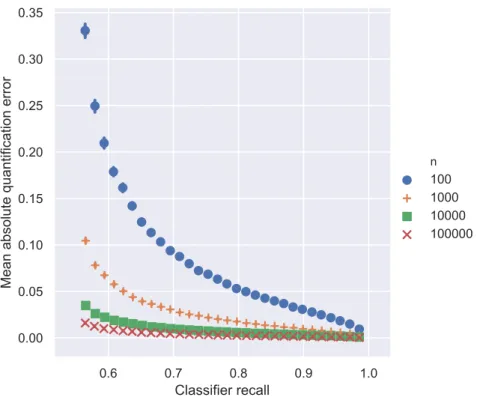
3.10 Mean absolute quantification error using classify and adjust method vs.
classifier recall and dataset size(n). Simulated data. . . 69
vii
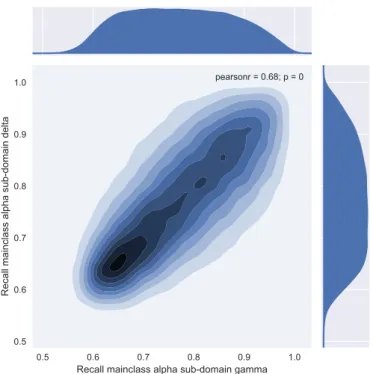
3.11 Kernel density estimation plot showing correlation of main-class α recall
values between the two sub-domains γ and δ . . . 71
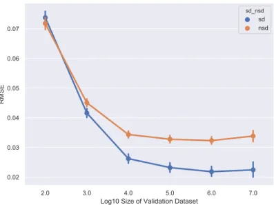
3.12 Quantification error in RMSE for the sd and nsd methods vs. log10 of validation set size . . . 72
3.13 Boxplot of ∆RMSE against size of validation set . . . 72
3.14 Kernel density estimation plot showing correlation of main-class α recall values between the two sub-domains γ and δ . . . 73
3.15 Boxplot ∆RMSE against size of validation set when main-class recall is the same in both sub-domains . . . 74
3.16 RMSE vs. main mainclass recall. 95% CI shown. . . 76
3.17 ∆RMSE vs. sub-domain recall mean . . . 77
3.18 ∆RMSE vs. Log10 of size of test set when validation set>10,000 . . . 77
4.1 Mean delta absolute error nsd-method minus absolute error sd-method by validation dataset size. 95% confidence intervals shown. . . 83
4.2 Mean delta absolute error (nsd-method minus absolute error sd-method) by quartile of bs prop prod. 95% confidence intervals shown. . . 84
4.3 Delta RMSE (nsd-sd) by quartile of bs prop prod and quartile of SDD . . . 85
4.4 Distribution of trv set sizes . . . 90
4.5 Classifier accuracy by dataset . . . 91
4.6 Mean delta absolute error nsd-method minus absolute error sd-method by decile of trv size. UCI dev datasets. 95% confidence intervals . . . 92
4.7 Mean delta absolute error nsd-method minus absolute error sd-method by decile of trv size. UCI dev datasets. 95% confidence intervals . . . 92
4.8 Mean delta absolute error nsd-method minus absolute error sd-method by decile of log10 c2p sum. UCI dev datasets. 95% confidence intervals . . . . 93
4.9 Mean delta absolute error nsd-method minus absolute error sd-method by decile of log10 c2p sum. UCI dev datasets. 95% confidence intervals . . . . 94
4.10 Mean delta absolute error nsd-method minus absolute error sd-method by absolute difference in sub-domain proportion between trv and te (SDDN). UCI dev datasets. 95% confidence intervals . . . 95
4.11 Distribution by estimated year of birth in the TAF training dataset . . . 103
5.1 Typical normalised distribution of the level of dataset shift in the test sets drawn from UCI dev, UCI test and TAF. Dataset shift measured by PADcb.111
5.2 Typical distribution of the level of dataset shift in the UCI dev datasets
test sets. Dataset shift measured by PADcb. . . 112
5.3 Typical distribution of level of dataset shift in the UCI test datasets test
sets. Dataset shift measured by PADcb. . . 112
5.4 Median cumulative weight proportion from KMM method vs. level of
dataset shift as measured by PADcb. Shown separately by dev dataset, kernel size multiple and B parameter . . . 114
5.5 Median cumulative weight proportion from uLSIF method vs. level of
dataset shift as measured by PADcb. Shown separately by dev dataset, kernel size multiple and B parameter . . . 115
5.6 Classifier accuracy by dataset . . . 119
5.7 Proportion of instance weight applied to class 0 instances in the training set
vs. proportion of class 0 instances in the test set. KMM method. UCI dev datasets. Kernel size multiples{0.01, 0.1, 1, 10}. . . 121
5.8 Proportion of instance weight applied to class 0 instances in the training
set vs. proportion of class 0 instances in the test set. UCI dev datasets.
uLSIF method. Sigma parameter {1.0, 3.162, 10.0} . . . 122
5.9 MAE of ut method with KMM weighting, threshold=0.5, kernel size
mul-tiple=1.0 and uu baseline method vs. PADcb quartile. UCI dev datasets. 95% confidence intervals . . . 129 5.10 MAE of ut method with KMM weighting, threshold=0.5, kernel size
mul-tiple=1.0 and uu baseline method vs. PADcb quartile. UCI test datasets. 95% confidence intervals . . . 130 5.11 Delta MAE of ut method with KMM weighting, threshold=0.5, kernel size
multiple=1.0. vs uu baseline method by PADcb quartile. 95% confidence intervals . . . 130 5.12 MAE of ut method with KMM weighting, threshold=0.7, kernel size
mul-tiple=1.0. and uu baseline method vs. PADcb quartile. UCI dev datasets. 95% confidence intervals . . . 131 5.13 MAE of ut method with KMM weighting, threshold=0.7, kernel size
mul-tiple=1.0. and uu baseline method vs. PADcb quartile. UCI test datasets. 95% confidence intervals . . . 132
ix
5.14 Absolute quantification error using classify and adjust method vs. class-conditional dataset shift. . . 137 5.15 ITTBR. PADcb by sub-iteration step. UCI dev datasets. . . 141 5.16 ITTBR. Absolute quantification error delta from initial value. Dev datasets.
95% confidence intervals . . . 141 5.17 Baseline absolute quantification error delta from initial value. Points
re-moved from training set at random. Dev datasets. 95% confidence intervals 142 5.18 ITTBR absolute quantification error delta from initial value less baseline
value. Dev datasets. 95% confidence intervals . . . 142 5.19 Absolute quantification error (actual vs. predicted class 0 proportion). Dev
datasets. . . 143
6.1 Mean mSDA calculation time per layer vs. number of data instances. 95%
confidence intervals shown. All UCI datasets . . . 149
6.2 RMSE of results from UCI dev datasets. mSDA layers from 0 to the layer
indicated. 95% confidence intervals shown. . . 153
6.3 RMSE of results from UCI dev datasets. mSDA layers from the layer
indi-cated up to and including layer 5. 95% confidence intervals shown. . . 153
6.4 RMSE of results from UCI dev datasets vs. level of noise. 95% confidence
intervals shown. . . 154
6.5 RMSE of results from UCI dev datasets. Impact of the balance of mSDA
training data between Source and Target domains. 95% confidence intervals shown. . . 155
6.6 Absolute quantification error vs. recall delta. mSDA results. UCI dev
datasets . . . 156
6.7 Recall delta vs. mSDA highest layer for mSDA results with UCI dev datasets.
Lowest layer = layer 0 . . . 157
6.8 Recall delta vs. mSDA lowest layer for mSDA results with UCI dev datasets.
Highest layer = layer 5 . . . 157
6.9 MAE of best mSDA method and baseline method vs. PADcb quartile.
UCI dev datasets. 95% confidence intervals . . . 158 6.10 MAE of best mSDA method and baseline method vs. PADcb quartile.
UCI test datasets. 95% confidence intervals . . . 158 6.11 MAE of ‘best’ method minus MAE baseline by PADcb quartile for UCI dev
6.12 MAE of ‘best’ method minus MAE baseline by PADcb quartile for UCI test datasets . . . 159 6.13 MAE of best mSDA method and baseline method vs. PADcb quartile. TAF
dataset. 95% confidence intervals . . . 161
List of Tables
2.1 Variations on theAdjusted Count method from Forman [44] . . . 9
2.2 Quantification loss functions . . . 15
2.3 Types of dataset shift [88] . . . 17
2.4 Reasons fordataset shift from Storkey [103] . . . 18
2.5 Importance weighting methods from Sugiyama and Kawanabe [104] . . . 27
2.6 Comparison of importance weighting methods [104] . . . 27
3.1 Class, main-class and sub-domain . . . 38
3.2 Key to symbols . . . 42
3.3 Class, main-class and sub-domain . . . 42
3.4 Observed recall values by main-class and sub-domain in the 4dSDA dataset 50 3.5 RMSE of sd and nsd methods . . . 51
3.6 Mean and variance sd and nsd method . . . 53
3.7 Class, main-class and sub-domain . . . 54
3.8 Numerical simulation: fixed parameter values . . . 70
3.9 Numerical simulation: sampled parameter values . . . 70
3.10 Numerical simulation: results of OLS regression using 6 parameters, full range of parameter values . . . 75
3.11 Numerical simulation: results of OLS regression using 6 parameters, nv > 10,000 . . . 75
4.1 Numerical simulation: fixed parameter values . . . 82
4.2 Numerical simulation: sampled parameter values . . . 82
4.3 Development datasets: UCI dev . . . 87
4.4 Held-out test datasets: UCI test . . . 87
4.5 Parameter settings . . . 90
4.6 Difference in abs error between nsd and sd-methods for various values of
baseline log10 trv size. UCI dev datasets . . . 96
4.7 Optimum multiple parameter values. UCI dev datasets . . . 97
4.8 Comparison of quantification performance of single and multiple criteria on the UCI dev datasets . . . 97
4.9 Combined UCI test datasets. Quantification performance with single and multiple criteria. . . 98
4.10 UCI CASP dataset. Quantification performance with single and multiple criteria. . . 99
4.11 UCI credit card default dataset. Quantification performance with single and multiple criteria. . . 99
4.12 UCI online news popularity dataset. Quantification performance with sin-gle and multiple criteria. . . 100
4.13 Proportion of results where the nmethod gives larger error than the sd-method . . . 101
4.14 Filtering applied in the generation of the TAF dataset . . . 103
4.15 Dimensionality reduction steps in the generation of the TAF dataset . . . . 104
4.16 TAF dataset split into tr, dev and te . . . 104
4.17 UCI online news popularity dataset. Quantification performance with sin-gle and multiple criteria. . . 106
4.18 Proportion of results where the nmethod gives larger error than the sd-method, TAF dataset . . . 106
4.19 TAF dataset. Quantification performance with single and multiple criteria. 107 4.20 Summary of Chapter 4 results . . . 108
5.1 Overall parameter settings . . . 117
5.2 KMM parameter settings . . . 118
5.3 uLSIF parameter settings . . . 118
5.4 Classifier kernel selection by dataset . . . 119
5.5 Approaches to introduce class-conditionality into instance weighting . . . . 124
5.6 Methods used to combine computed instance weights with the matrix-inversion quantification method . . . 125
5.7 Method-parameter settings with lower MAE than baseline which are sta-tistically significant at α < 0.05 under the Friedman test with Bonferroni corrections. UCI dev datasets. . . 127
xiii
5.8 Best method by mean rank from Table 5.7 . . . 127
5.9 Performance of best method from UCI dev datasets on the held-out UCI test
datasets . . . 128 5.10 Best method-parameter by MAE on UCI dev datasets for both KMM and
uLSIF instance weighting . . . 133 5.11 Best SSBC methods by mean rank, RMSE and MAE. UCI dev datasets . . 135 5.12 Best SSBC methods by mean rank, MAE and RMSE. UCI test datasets . . 136 5.13 ITTBR parameter settings . . . 139 5.14 Summary of Chapter 5 results . . . 145
6.1 Ten feature representations plus baseline constructed from the original
fea-tures (layer 0) and the five mSDA layers . . . 150
6.2 Best mSDA methods on UCI dev datasets against mean rank, RMSE and
MAE . . . 152
6.3 Best mSDA methods from UCI dev measured on the UCI test datasets . . . 152
6.4 RMSE from best method on UCI dev datasets vs. baseline for varying tr
and te set sizes . . . 155
6.5 Best mSDA methods from UCI dev measured on the TAF dataset . . . 160
6.6 Best mSDA methods on TAF dataset against mean rank, RMSE and MAE 160
6.7 Summary of Chapter 6 results . . . 161
7.1 Summary of results . . . 164
7.2 Size of validation set above which the sd-method gave better quantification
Variables
Style Example Use
Italic Roman lowercase nt Scalars
Bold Roman lowercase avs Vectors
Italic Roman uppercase P Random Variables
Roman uppercase R∗ Matrices
xv
av Vector of actual counts by class (main-class and sub-domain) in the
validation dataset
at Vector of actual counts by class (main-class and sub-domain) in the test
dataset
ant Vector of actual counts by class (main-class only) in the test dataset
R∗ Matrix of actual-to-predicted class probabilities implicit in the classifier
Rv Matrix of actual-to-predicted class (main-class and sub-domain) ratios
as observed for the validation dataset
pv Vector of predicted counts by class (main-class and sub-domain) as
gen-erated by the classifier from the validation dataset
Rnv Matrix of actual-to-predicted class (main-class only) ratios as observed
for the validation dataset
pt Vector of predicted counts by class (main-class and sub-domain) as
gen-erated by the classifier from the test dataset
pnt Vector of predicted counts by class (main-class only) as generated by
the classifier from the test dataset ˆ
at Vector of estimated actual counts by class (main-class and sub-domain)
for test dataset using sub-domain method ˆ
atm Vector of estimated actual counts by class (main-class only) in the test
dataset using sub-domain method ˆ
ant Vector of estimated actual counts by class (main-class only) in the test
dataset using no-sub-domains method
esd Error between estimated and actual class counts in the test dataset from
method using sub-domains
ensd Error between estimated and actual class counts in the test dataset from
method not using sub-domains
nv The size of the validation dataset
Introduction
How do you accurately estimate the class proportions in a dataset when the class-conditional feature distribution is different to that of the dataset that is available for training?
Often it is not the class ofindividual data points that is of interest, it is thedistribution of classes in the whole dataset. In sentiment analysis it might be the proportion of a group that is positive about a product. In market research it might be the ratio of men to women in a group of respondents and in epidemiology it might be the prevalence of a disease in a population. Increasingly, the requirements for privacy and anonymity mean that analysis has to be presented as group aggregates with any information at individual level removed. Estimating the class distribution in a dataset instead of the classes of individual data
points has been termed quantification [42].
The na¨ıve approach (classify and count) is simply to classify the data with a classifier
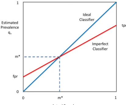
and count the number of instances assigned to each class. However this approach is flawed because classifiers are imperfect. Consider Figure 1.1. Given a test sample that is made up of 100% positive instances, a classifier will only classify some of those instances as positives. The proportion of actual positive instances that are classified as being positive is the True
Positive Rate (tpr). Similarly when the test sample is made up of 100% negative instances,
a classifier will inevitably classify some of those instances as positives. The proportion of actual negative instances that are classified as positive is the False Positive Rate (fpr).
For some value of class distribution m∗ the number of false negatives will exactly offset
the number of false positives and the estimated class distribution will be correct. For all
2
other class distributions the estimate will be incorrect.
tpr Estimated Prevalence q+ m* fpr 1 1 0 0 m* Actual Prevalence m+ Ideal Classifier Imperfect Classifier
Figure 1.1: Estimated and actual class distribution with theclassify and count method
This can be relatively simple to correct. Classify and adjust methods apply an adjustment
to the output of the classifier that corrects for its imperfect classification. Figure 1.2 shows
the quantification performance of a classify and count method and a classify and adjust
method. The estimates from the classify and count method are as would be expected
from Figure 1.1 while the improvement in estimation accuracy from theclassify and adjust
method is clear.
Classify and adjust methods typically require the assumption that the performance of the
classifier on each class in the test data is the same as it was on each class in the original labelled training data. This implies that the class-conditional feature distribution in the test data, Pte(x|y), is the same is it is in the training data, Ptr(x|y). As per the usual
convention,x represents the features of the data while y represents theclass labels.
However, the class-conditional feature distribution maynot the same in both the training
and test sets, for example:
A ‘quantifier’ has been trained to give an estimate of the male/female gender balance in a group of individual Twitter users based on the accounts that they are following on Twitter. The quantifier has been trained with a broad set of UK Twitter users with each user correctly labelled as male or female. The quantifier is then used to estimate the gender
0.0 0.2 0.4 0.6 0.8 1.0
Actual class proportion
0.0 0.2 0.4 0.6 0.8 1.0
Estimated class proportion
Method
Classify and Adjust Classify and Count Actual
Figure 1.2: Estimated vs. actual class proportions using both theclassify and count and
theclassify and adjust methods. UCI dev datasets. Data from Section 5.9
balance of another group of individuals. This group of individuals have all been selected because they tweeted about retirement homes in Scotland.
This group of Twitter users, selected from a population on the basis of the content of what they say in a tweet, are unlikely to have the same class-conditional feature distribution as the group of users on which the quantifier was trained. In this example, within each class (male and female) the age and location distribution of the dataset in question is likely to be different. This differencecould result in an error in the estimation of the gender balance
of the group. In general, wecannot simply assume that a dataset that has been generated
as a result of some selection process has the same class-conditional feature distribution as the dataset on which the quantifier was originally trained.
When class-conditional feature distributions are different we refer to this as class-conditional
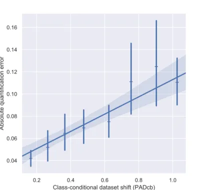
dataset shift. Figure 1.3 shows how quantification accuracy with a standardclassify and
adjust method degrades with increasing class-conditional dataset shift1.
The majority2 of academic work on quantification makes the assumption that
class-1
see Section 5.1 for an explanation of PADcb 2
4
0.2 0.4 0.6 0.8 1.0
Class-conditional dataset shift (PADcb)
0.04 0.06 0.08 0.10 0.12 0.14 0.16
Absolute quantification error
Figure 1.3: Absolute quantification error using classify and adjust method vs. class-conditional dataset shift. Data from Section 5.9. 95% confidence
intervals.
conditional dataset shift hasnot occurred. The novelty in this thesis is that its focus is on
quantification when class-conditional dataset shifthas occurred. Its main contribution is
to demonstrate that several approaches can reduce quantification error under conditions of class-conditional dataset shift. The best of these, using importance weighting to select from the labelled validation data, gave a relative improvement in quantification error of
10.7% over theclassify and adjust baseline on datasets where the class-conditional feature
distribution is different from that of the training data.
In this thesis, three different approaches are applied to the problem of quantification
under class-conditional dataset shift: explicit sub-domains in Chapters 3 and 4;importance
weighting of instancesin Chapter 5 andfeature representations in Chapter 6. However, all
of these methods fundamentally address the problem in a similar way: applying adomain
adaptation step to reduce (or ideally eliminate) the class-conditional feature distribution
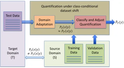
difference between the training and test sets so that a standard quantification method that relies on the assumption of no change in class-conditional feature distribution can work effectively. This is shown diagrammatically in Figure 1.4.
Classify and Adjust Quantification Domain Adaptation !" # $ ≠ !& # $ !" # $ ≈ !& # $
Quantification under class-conditional dataset shift Validation Data Source Domain (S) Target Domain (T) ( !&($) Training Data Test Data
Figure 1.4: Common approach to quantification under class-conditional dataset shift
Theexplicit sub-domains approach in Chapters 3 and 4 can be thought of as a ‘divide and
conquer’ approach. In these chapters the assumption is made that the data can be broken down into smaller groups (‘sub-domains’) in which the conditional feature distributions
do not vary. Quantification is carried out at this sub-domain level and the results then
aggregated up to class level as a final step. A limitation of this method is that the sub-domain has to be identified up-front and labelled in the training data. Another drawback of this approach is that dividing the training set into smaller groups increases the relative level of ‘noise’. The question explored in these chapters is whether the advantages of quantifying in smaller sub-domains outweighs the disadvantages from increased noise. An analytic approach yielded a closed-form answer to this question but only when the assumption was made that there is a large amount of labelled data available at training time. Numerical simulation allowed the question to be explored without making simplifying assumptions and showed the significance of a number of parameters.
In Chapter 4, the insights from Chapter 3 are used to develop a method which utilises sub-domains only when doing so was likely to improve quantification accuracy. This method achieved a 4.5% relative improvement in mean absolute error over the baseline method on the test data.
In Chapter 5, importance weighting of instances methods are used for domain
adapta-tion. With these methods, the distribution of the training data is brought closer to the
distribution of the test data by applying ‘importance’ weights to individual instances in the training set. Several methods of computing importance weights are used including Sample Selection Bias Correction [122], Kernel Mean Matching [58] and Unconstrained
6
Least-Squares Importance Fitting [104]. These methods work on aligning data
distri-butions overall, not specifically the class-conditional distribution differences, so various
approaches were taken to address the issue of class-conditionality. Ultimately, a method using Kernel Mean Matching gave a 10.7% relative improvement in mean absolute error over the baseline method on the test data.
In Chapter 6, attention switches from instances to features. Domain adaptation is
ad-dressed by using the Marginalised Stacked Denoising Autoencoder (mSDA) method [29] to transform the original features into a new representation. The best paramater settings gave a 3.3% relative improvement in mean absolute error over the baseline method on the test data.
The relevant literature is reviewed in Chapter 2 and conclusions and directions for potential further work are set out in Chapter 7.
The motivation for this work came from the Polly project in 2014-15. The Polly project was a collaboration between the University of Sussex, CASM Consulting LLP, the market research firm Ipsos-Mori and the think-tank Demos. It was funded by the UK Technology
Strategy Board (now Innovate UK), the EPSRC3 and the ESRC4. A key part of the
project was to explore the potential for the demographic profiling of Twitter users and promising results were obtained for estimating age, gender and location. The question of a dataset shift between the dataset being tested and the dataset on which the classifiers were trained was acknowledged as a possible issue but was not explicitly addressed as part of the project.
3The Engineering and Physical Sciences Research Council 4The Economic and Social Research Council
Literature review
This Chapter is organised into four sections. Literature on quantification is explored in
Section 2.1, dataset shift in Section 2.2 and unsupervised domain adaptation in Section
2.3. Finally, literature that has brought togetherdomain adaptation and quantification is
reviewed in Section 2.4.
Throughout the thesis, data that is used for training purposes is referred to as thetraining
set and we say that it has been drawn independently and identically distributed (iid) from
theSourcedomain. Similarly, we say that the data that is used for testing purposes is the
test set which has been drawn iid from theTarget domain.
2.1
Quantification
The approaches to quantification can be grouped into four broad categories:
• Classify and count
• Classify and adjust
• Distribution matching
• Direct quantification
8
2.1.1 Classify and count
For the reasons outline in the Introduction, classify and count is a na¨ıve approach to
quantification. The inevitable imperfection of the classifier gives an inevitably imperfect method of estimating class proportions.
2.1.2 Classify and adjust methods
Classify and adjust methods still rely on a trained classifier to classify or assign class
probabilities to the data but then a second adjustment step is applied to arrive at the
actual estimate of class proportions. The adjustment step implicitly or explicitly relies on information about the relationship between the actual and estimated class labels that has been obtained from labelled data, typically at the time that the classifier is trained. The two most common approaches to making this adjustment are matrix-inversion and probabilistic expectation-maximisation.
2.1.2.1 Matrix-inversion
The error from the classify and count method can be corrected with a simple linear
transformation. Assume we have two classes, positive (+) and negative (-). The test
set contains nt instances of which a+ are in the positive class. We define m+ as the
proportion of actual positive class instances in the test set: m+=
a+
nt
, (2.1)
and ˆm+ as the estimate of this value. Counting the instances by predicted class as given
by the classifier (i.e. the classify and count method) we havep+ positives. We define q+
as the proportion of predicted class positive instances in the test set where: q+=
p+
nt
. (2.2)
The matrix-inversion estimate of m+ is then [42]:
ˆ m+ =
q+−fpr
tpr−fpr, (2.3)
where the True Positive Rate (tpr) and False Positive Rate (fpr) are calculated from
has not been used to train the classifier. This method relies on the assumption that the
computed tprand fpr values are the same as would be seen on the test data if its labels
were available for inspection i.e. that the class-conditional feature distribution in the
Target domain is thesame as that in the Source domain.
In the field of machine learning, the matrix-inversion method is usually credited to Forman
[42] as theAdjusted Count method, although this is fundamentally the same method that
was seen earlier in Vucetic and Obradovic [117]. In epidemiology this method has been used since at least the 1960s. Rogan and Gladen [95], Levy and Kass [81] and Buck et al. [21] are widely cited.
Forman [44] puts forward a range of variations on the Adjusted Count method that are
aimed at prioritising quantification performance over classification performance. These are shown in Table 2.1.
Table 2.1: Variations on the Adjusted Count method from Forman [44]
Method Description
Crossover Set the threshold of the classifier such that it givesfpr= (1−tpr)
T50 Select the classifier threshold that results intpr = 50%
Max Select the classifier threshold that results in the maximisation of
the denominator i.e. maximise (tpr - fpr)
Median Sweep Compute ˆm+foreverysetting of the classifier threshold and return
themedian of these values
Forman [44] observes that Median Sweep performs better than the Mixture Model and
Adjusted Count methods although he suggests though that T50 and Crossover may be
simpler to implement.
While many further works discussed in this section claim to have achieved higher levels of performance, the performance of the simple matrix-inversion method has proved to be strong. It has frequently been used as a baseline and has frequently been shown to perform on a similar level to the author’s own chosen approach (e.g. Barranquero et al. [12] Esuli and Sebastiani [37] Gao and Sebastiani [49] Milli et al. [86] Xue and Weiss [121]). Gonz´alez et al. [52] states that the AC method is a theoretically perfect method when its learning
assumptions are fulfilled i.e. if we have perfect estimates for tpr and fpr for the data on
10
Bella et al. [13] put forward a variation onAdjusted Count method which they calledScaled
Probability Average. They believe that class-probabilities offer richer information on the
dataset than estimated class labels. In this method the aggregated class probabilities from a classifier are first computed and then are adjusted in a similar manner to the way that
Forman [44] adjusts the counts by class with theAdjusted Count method. Bella et al. [13]
found that theirScaled Probability Averagemethod outperformed other methods including
the Forman [44] Adjusted Count method. However, Esuli and Sebastiani [37] performed
a number of tests and found that Scaled Probability Average was not consistently better
thanAdjusted Count.
Further details of the Forman [42]Adjusted Count method can be found in Section A.1
2.1.2.2 Probabilistic expectation-maximisation
In 2002 Saerens et al. [97] outlined a probabilistic expectation-maximisation method for estimating class distribution that is considered to be seminal [35] and arguably the most popular algorithm for quantification [52].
The method requires a classifier that generates an output that can be interpreted as the
probability of being a member of each class, P(y|x). In the matrix-inversion method
above, the information about the probabilistic relationship between actual and predicted
class labels is explicit in the values of tpr and fpr. In this method this information is
implicit in the training of the classifier and the class label probabilities that it assigns.
The classifier is trained on the labelled training data and then used to assign estimated
class probabilities to the test data from the Target domain, PT(y|x). After that a two
step adjustment process iterates until a convergence criteria is met:
1. The class distribution PT(y) is re-estimated by marginalising the latest estimate of
posterior class probabilities PT(y|x).
2. The posterior class probabilities PT(y|x) are re-estimated using the latest estimate
of the class-distributionPT(y).
2.1.3 Distribution matching
The observed distribution of features, PT(x), or estimated class probabilities, PT(ˆy), in
the Target domain is assumed to be a mixture of the class-conditional feature distributions in the Source domain observed at training time.
The class distribution in the Target domain is estimated by comparing the test set to a synthetic dataset which has been made up by sampling the labelled data from the Source domain to a given class proportion. The estimate of the class proportion in the Target domain is the class proportion in the synthetic set which minimises some measure of distance between the distribution of the synthetic set and the distribution of the test set. Different authors have used different distance metrics.
Clearly these methods are again dependent on the assumption that the class-conditional feature distribution is the same in the Source and Target domains.
2.1.3.1 Distribution matching in the estimated label space Yˆ
Forman [42] put forward the Mixture Model method. Firstly, a classifier is trained with
data from the Source domain, then other labelled data from the Source domain is put through the trained classifier to give a distribution of raw classifier output values for each class.
Forman [42] uses a measure he defines as PP-Area to measure the distance between the
test and the synthetic datasets. PP-Area is defined as the area bounded by the Cu-mulative Distribution Function (CDF) of the test dataset and the CDF of the synthetic dataset. Forman [42] considered PP-Area to be a better metric than the more
conven-tional Kolmogorov-Smirnov value. He found thatMixture Model was very resilient to wide
variations in the class distribution of the training data, but was normally outperformed
by the variants on theAdjusted Count method (Crossover,T50,Max,Median Sweep (see
Section 2.1.2.1)).
Gonz´aLez-Castro et al. [54] measured the distance between the two distributions using
Hellinger Distance. They found that estimating class proportions with a method based
on the predicted class labels ˆy performed better than the method based the feature
12
2.1.3.2 Distribution matching in the feature space X
Du Plessis and Sugiyama [35] showed that the Saerens et al. [97] EM algorithm can be re-fomulated as a mixture method which minimises Kullback-Liebler (KL) divergence. They, however, prefer Pearson (PE) divergence to KL-divergence as the measure to minimise. PE-divergence can be considered to be the squared-loss variant of KL-divergence [35]. They prefer PE-divergence largely for reasons of practical implementation but also state that it has superior convergence properties. There was some difference in performance for the five methods that they implemented when they were applied to the six datasets, but in all six cases the PE-divergence based method either equalled or was better than the Saerens et al. [97] EM method.
As discussed above, Gonz´aLez-Castro et al. [54] explored distribution matching by
min-imising the Hellinger Distance in both the estimated label space ˆY in the previous section,
and in the feature space X. They obtained better performance when working in ˆY and
be-lieved that the lower performance in X was down to the issue of sparseness. The approach taken by Du Plessis and Sugiyama [35] and Iyer et al. [68] to measuring distance in X is
ar-guably more sophisticated than the Hellinger distance approach used by Gonz´aLez-Castro
et al. [54] and this may explain its superior performance.
2.1.3.3 Distribution matching in a transformed feature space
Iyer et al. [68] and Kawakubo et al. [76] projected the distributions into a Reproducing-Kernel Hilbert Space (RKHS) and then minimised Maximum Mean Discrepancy (MMD) (see Section 2.2.3.2). Their work builds on previous work such as Saerens et al. [97], Du Plessis and Sugiyama [35] and Zhang et al. [124]. Iyer et al. [68] initially used the PE-divergence method favoured by Du Plessis and Sugiyama [35] as a baseline, but dropped it stating that it (surprisingly) performed no better than a baseline of counting by predicted class using a classifier built on the work of Sun et al. [107].
2.1.4 Direct quantification
Given that the ultimate aim isquantificationand notclassificationan alternative approach
is to learn aquantifier directly and not to learn a classifier as an intermediate step. This
on classification error.
Esuli and Sebastiani [37] [38], Barranquero et al. [12] and Gao and Sebastiani [49] [48] all
used the SVM for Multivariate Performance Measures (SVM∆multi) method as put forward
by Joachims [72]. This method is itself a development from Tsochantaridis et al. [111]. Classifiers typically minimise a loss function where the loss is aggregated from the losses
computed for each individual instance in the training set. Joachims [72] SVM∆multi method
is different in that it can minimise a loss function that has been computed across a set
of data instances where the loss cannot be dis-aggregated to a loss for each instance, for
example from a confusion matrix. This allows a classifier to be trained to directly optimise a measure of quantification accuracy.
Esuli and Sebastiani [37] [38] use the Kullback-Leibler divergence (KLD) for their loss function. Specifically the KLD between the actual class distribution and the predicted class distribution based on the count of instances by predicted class from the classifier. They compare this method (which they term SVM(KLD)) to other baseline methods such as those of Forman [44] and Bella et al. [13] and claim that it is superior in accuracy, stability and running time.
Interestingly they comment that tpr and fpr were far from invariant across different sets
and they argue that this supports the SVM(KLD) method over methods such asAdjusted
Count that require explicit values for tpr and fpr. However, SVM∆multi / SVM(KLD) is
still optimising over the full set of training data. The assumption is that the test set and the training set are be drawn iid from the same domain. The SVM(KLD) will have learnt
some relationship between the set of x values of the instances in the training set and the
set of class labelsy. While the method does not rely onexplicit values for tpr and fpr it
will be just as susceptible to the underlying changes in the relationship between x and y
that cause those changes in tpr andfpr.
Barranquero et al. [12] also implemented a similar quantification approach to that used by Esuli and Sebastiani [37] i.e. one based solely on quantification loss. They found that
it performed poorly. They argue that in order to generalise well a quantifier must still
be a good classifier. A loss function that only focuses on quantification error (such as is
the case with Esuli and Sebastiani [37]) is, in their view, unsuitable because the resulting hypothesis space contains several local optima. Like Esuli and Sebastiani [37] they also
14
quantification loss functionanda classification loss function1. However, when they applied
the analytical approach as advised in Demˇsar [31] they found no statistically significant
difference between this method and 6 of the 7 Forman [44] methods that were used as benchmarks.
One possible explanation for the better performance claimed by Esuli and Sebastiani [37] is that their experiments used a large number of classes (88 in one experiment and 99 in another) whereas the Barranquero et al. [12] experiment used binary classes. As the number of classes tends towards the number of data instances (i.e. to a point where each class contains just one data instance and vice versa) the error in the estimate of class distribution (the quantification error) tends towards the classification error. By choosing such a large number of classes Esuli and Sebastiani [37] are effectively incorporating a degree of classification loss into their quantification loss based approach.
Tasche [109] looked at both the Barranquero et al. [11] and Esuli and Sebastiani [37] direct quantification methods and evaluated the method from Barranquero et al. [11] both from a theoretical perspective and experimentally. He found that the method was sensitive to mis-calibration and limited in its application.
Milli et al. [86] put forward a direct quantification method that did not make use of
the Joachims [72] SVM∆multi. Their method used decision trees (Quantification Trees).
They reported better performance than the Forman [44]Adjusted Countmethod, although
in several cases the Adjusted Count method actually gave the best performance. The
baselines forAdjusted Countused classifiers with the parameters set at their default values. Finally, the class distribution of the training sets was varied between 0.05 and 0.95. There are known issues when using unbalanced datasets to train standard classifiers [26] [69] [79] and this may have a larger negative impact on the baseline SVM classifier than on their decision tree method. However, despite these reservations, there is the possibility that their method is somehow akin to building a robust feature representation as per the methods set out in Section 2.3.3 and would potentially be an interesting area for further work.
In summary, Barranquero et al. [12] re-implemented the method from Esuli and Sebastiani [37] and found it performed poorly but found that their own method is not statistically
1
significantly better than the methods from Forman [44]. Tasche [109] also found that their method was no better than simple classify and adjust methods such as those from Forman [44]. Finally, the method in Milli et al. [86] was also not found to be clearly superior to the methods from Forman [44].
My conclusion was that none of the direct quantification methods are demonstrably
supe-rior than the far simplerAdjusted Count method from Forman [44] so this is the method
chosen for use in this thesis.
2.1.5 Quantification loss functions
The distribution matching methods in Section 2.1.3 and the direct quantification methods in Section 2.1.4 minimise a loss function over a set of instances rather than aggregate a loss function calculated separately for each instance in a set. Different authors have used a variety of loss functions, some of which are listed in Table 2.2 below:
Table 2.2: Quantification loss functions
Title Used in Note
NSS Normalised Square Score [12]
NAS Normalised Absolute Score [12]
EMD Earth Mover’s Distance [62] [76] see 2.2.3.3
HDx Hellinger Distance in X [54]
HDy Hellinger Distance in y [54]
PE Pearson Divergence [35]
MMD Maximum Mean Discrepancy [68] [76] see 2.2.3.2
PP-Area PP-Area [44]
2.1.6 Quantification test methods
The normal method (e.g. Forman [44], Bella et al. [13], Barranquero et al. [12]) for testing for quantification accuracy is to construct test datasets of a given class distribution by separately sampling instances of each class from the available labelled data. This is the approach I have used.
16
without any adjustment to the class proportions. They argue that artificially adjusting
class proportions would create unrealistic datasets. Gonz´alez et al. [52] are sympathetic
to this approach, observing that the class-conditional sampling methods may be artificial with respect to the actual data distribution of the problem.
This is an interesting question for further work and is discussed further in Chapter 7.
2.1.7 Quantification applied to specific areas
In many papers the motivation to explore quantification is driven by a particular problem in a particular field.
In epidemiology, estimating disease prevalence using screening tests is effectively the
equiv-alent ofquantification in computer science [87]. The limitations of the simpleclassify and
count method with an imperfect test are well known and the matrix-inversion formula
that computer scientists credit to Forman [42] in 2005 has been used by epidemiologists for estimating disease prevalence since Rogan and Gladen [95] in 1978, Levy and Kass [81] in 1970 or Buck et al. [21] in 1966.
However, while epidemiologists have been working with the problem of quantification with imperfect classifiers for many years (e.g. Cowling et al. [30], Donald et al. [33], Greiner and Gardner [56], Joseph et al. [73], McV Messam et al. [85]) they do not appear to have developed methods for dealing with quantification under dataset shift that could be used as part of the work for this thesis.
In social science, Hopkins and King [65] point out that practitioners want generalisations about the population of documents rather than the classification of individual documents i.e. quantification rather than classification. The focus of their work is on quantifying electronic records (blogs, speeches, government records, newspapers etc.) by category. Finally, sentiment analysis is an area which features heavily in the works on quantification. Works in this area include Blitzer et al. [19], Chan and Ng [25], Esuli et al. [38], Amati et al. [6], Chan and Ng [24] and Gao and Sebastiani [48]. By its nature, users of sentiment analysis tend to be interested in the aggregate opinion of a group rather than the opinion of individuals.
2.2
Dataset shift
Dataset shift is when the joint distribution between featuresx and labels y in the Target
domainT differs from that in the Source domainS [93] i.e.
PT(x, y)6=PS(x, y) (2.4)
Bayes’ rule gives:
P(x, y) =P(x|y)P(y) =P(y|x)P(x). (2.5)
Using Bayes’ rule, Moreno-Torres et al. [88] put forward the taxonomy for types of dataset shift shown in Table 2.3.
Table 2.3: Types of dataset shift [88]
Conditional Marginal
Prior probability shift: PT(x|y) =PS(x|y) PT(y)6=PS(y)
Covariate shift: PT(y|x) =PS(y|x) PT(x)6=PS(x)
Concept shift: PT(x|y)6=PT(x|y) PT(y) =PS(y)
or PT(y|x)6=PT(y|x) PT(x) =PS(x)
Other shift: PT(x|y)6=PT(x|y) PT(y)6=PS(y)
or PT(y|x)6=PT(y|x) PT(x)6=PS(x)
Most works on quantification assume Prior Probability Shift [68] i.e. that while the class
distribution is different in the Target domain to the Source domain PT(y) 6= PS(y), the
class-conditional feature distributions are not i.e. PT(x|y) =PS(x|y).
In this thesis, the assumption is that the class-conditional feature distribution P(x|y) is
not the same in both the Source and Target domains. Assuming both thatPS(y)6=PT(y)
and PS(x|y) 6=PT(x|y) would be classified as other dataset shift in Moreno-Torres et al.
[88]. They regard these problems are so hard that they are currently ‘impossible’ to solve. However, several works have attempted to address this ‘impossible’ problem, typically by applying some form of constraint between the Source and Target domain.
18
2.2.1 Causality and dataset shift
Both Moreno-Torres et al. [88] and Storkey [103] link type of dataset shift to the direction of causality. A common point of reference for both is Fawcett and Flach [39], which is itself a response to Webb and Ting [118]. Moreno-Torres et al. [88] states that writing the joint
distribution as P(x|y)P(y) applies only to Y → X problems. However Gonz´alez et al.
[53] think that this is not correct. Their view is that the property that P(x|y) remains
unaltered must be analysed for each particular application, independently of whether it
belongs to X→Y orY →X problems.
2.2.2 Causes of dataset shift
Storkey [103] considered the reasons for dataset shift and proposed the six categories given in Table 2.4 below:
Table 2.4: Reasons fordataset shift from Storkey [103]
Simple Covariate Shift Only the distributions of X change, everything else stays the same
Prior Probability Shift Only the distribution of Y changes, everything else stays the same
Sample Selection Bias Distributions differ as a result of an unknown sample rejection process
Imbalanced Data Deliberate dataset shift for computational or modelling convenience
Domain Shift Changes in measurement
Source Component Shift Changes in strength of contributing components
While these are given as causes for dataset shift, they are in reality a mix of causes and types. Moreno-Torres et al. [88] makes a clearer separation of causes and types. They state that while there are a variety of potential causes the most important causes of dataset
shift aresample selection bias andnon-stationary environments.
Sample selection bias is itself a major area of study. With over 27,000 citations Heckman
[60] is regarded as the seminal work on the subject and is the field of study for which he won the Nobel prize in Economic Science. Zadrozny [122] applied Heckman’s methods
for correcting for sample selection bias to the world of machine learning and these are discussed in Section 2.3.2.1.
The concept of sample selection bias is very relevant to this thesis. Going back to the
motivating in Chapter 1, sample selection bias has occurred because the group of
individ-uals that we are looking to quantify have been selected on the basis of the content of their tweets. They are not a simple random iid sample of Twitter users.
By non-stationary environments, Moreno-Torres et al. [88] are considering environments
where the data is non-stationary intimeor non-stationary inspace. They give the example
of junk mail as an example of a non-stationary environment in time. The creators of junk mail change the content and format of the junk mails they generate to attempt to defeat advances in junk mail filtering. Kelly et al. [77], Gama et al. [45] and others address dataset shift as temporally non-stationary environment problem and in this area the term
drift is typically used.
Sample selection bias andnon-stationary environments can be seen as two ways of looking
at the same issue: non-stationary environments can be considered as the equivalent of
sample selection bias where the data in the Target domain has been sampled withsample
selection bias biased on either time or on space.
2.2.3 Measures of dataset shift
Measuring the shift between datasets is not a trivial problem. The three main approaches appear to be:
• A-distance
• Maximum Mean Discrepancy
• Earth Mover Distance
2.2.3.1 A-distance
A-distance was originally defined in Kifer et al. [78] where they state that the intuitive
meaning ofA-distance is that it is the largest change in probability of a set that the user
cares about. The authors were looking for a distance function that would detect a distance > between two distributions P1 and P2 with a sample of at most n points from each
20
of P1 and P2. They considered, and rejected several existing measures. They rejected
Jensen-Shannon Divergence because it can only be applied to discrete distributions and because they felt that the concepts of entropy on which it is built are hard to convey to end users. They rejected other common measures of distance between distributions because they are too sensitive (e.g. L1) or too insensitive (e.g. Lp withp >1)2.
However, the authors state that in practice, computing the exactA-distance is impossible
and that one has to compute a proxy. Ben-David et al. [14] showed that a proxy for A
-distance can be found by optimising a classifier to discriminate between the two datasets and observing the error.
ProxyA-distance ˆdA is defined as:
ˆ
dA= 2(1−2), (2.6)
whereis the error rate obtained with the best hypothesis from the hypothesis set.
This has an intuitive meaning: if an optimised classifier cannot distinguish between two equal-sized datasets then they are close. In this case the classifier error rate will be around 0.5 giving a ˆdA of around 0.
Using classification accuracy as a measure of dataset shift was also used by Torralba and Efros [110] to measure the similarity between image datasets. Similarly the sample selection bias correction method from Zadrozny [122] uses a classifier that is trained to distinguish between two datasets.
A-distance is a popular measure in the literature, probably because it can be computed
simply, has an intuitive meaning and is theoretically grounded.
Some recent works on domain adaptation have either used A-distance in their analysis
(e.g. Glorot et al. [50]) or have used it as a fundamental part of an adversarial learning approach (e.g. Ajakan et al. [4], Ganin et al. [47]).
2.2.3.2 Maximum Mean Discrepancy (MMD)
The concept behind Maximum Mean Discrepancy (MMD) is to take samples from the two domains in question and project the data in the samples into a Reproducing Kernel
2There is more discussion onL
Hilbert Space (RKHS) using a kernel function. The MMD test statistic is the difference between the mean values of the domain samples computed in the RKHS. The smaller the test statistic the more likely it is that the two samples were drawn from the same domain i.e. the more similar the domains. Maximum Mean Discrepancy is defined in Borgwardt et al. [20] and Gretton et al. [57].
Under certain circumstances MMD is equivalent to the metric of Energy Distance [98]. Energy distance is a statistical distance between the distributions of random vectors, which characterizes equality of distributions [108].
MMD has been used in a variety of works on dataset shift and domain adaptation including Hoffman et al. [64], Long et al. [82], [83], Pan et al. [91]. Interestingly MMD has also
been used for straightforward quantification but always under the prior probability shift
assumption that class-conditional feature distributions are the same in both the Target and Source domains e.g. Iyer et al. [68], Kawakubo et al. [76].
2.2.3.3 Earth Mover Distance (EMD)
Earth Mover Distance (EMD) was first introduced by Rubner et al. [96] [62]. It is
con-ceptually very similar to Wasserstein3 distance. EMD and Wasserstein distance are the
same when the two distributions being compared have equal mass [80]. EMD is popular measure for distributional similarity in the field of image processing (e.g. Rubner et al. [96]) but has also been used in other areas of dataset shift and domain adaptation (e.g. Hofer [62])
EMD is based on the concept of computing the minimal cost to transform one distribution to another and is effectively a transport problem [96]. As such the concept of ground distance is fundamental. In 2D images where pixels are features, ground distance has a natural physical meaning. In Hofer [62], Euclidean distance in the feature space is used as the measure for ground distance.
3
22
2.3
Unsupervised domain adaptation
Methods that addressdataset shift typically go under the heading ofdomain adaptation.
In this thesis we are only interested in unsupervised dataset shift i.e. when labelled data
is only available from the Source domain and not from the Target domain.
Very commonly, researchers have been addressing situations where they have a classifier that has been trained with data from one domain and then want to perform the same classification task in a similar but non-identical domain where the amount of labelled data is limited or non-existent. There is the strong intuition that they should still try to use knowledge obtained from the original domain, but to adapt it to the new domain.
Domain adaptation is also referred to as transductive transfer learning itself a subset
of transfer learning [90] [106]. Storkey [103] notes that ‘the problem of dataset shift is
closely related to another area of study known by various terms such as transfer learning
orinductive transfer’.
Domain adaptation is of particular interest in the fields of natural language processing (NLP) and image processing.
Approaches to unsupervised domain adaptation can be broadly categorised into four groups:
• Mixtures of sub-domains
• Importance weighting of instances
• Feature representations
• Weakly supervised
Domain adaptation is a very large area of study. In this literature review I have focussed on selected papers that are particularly relevant to the quantification under class-conditional dataset shift problem.
2.3.1 Mixtures of sub-domains
With mixture of sub-domain methods, the assumption is that the Source and Target
domains are both made up from a mixture of common sub-domains. While the class-conditional feature distribution differs between Source and Target domains the assumption
is that it doesnot vary within the sub-domains. The difference in class-conditional feature distribution between the Source and Target domains is then assumed to be fully accounted for by a difference in their constituent proportions of sub-domains.
2.3.1.1 Ensemble approaches
Broadly, in ensemble approaches, a classifier is trained specifically for each sub-domain and the overall output (say instance classification) is computed as a function of the outputs of the ensemble of classifiers. Works in this area include Mansour et al. [84] and Duan et al. [36].
2.3.1.2 Latent domains
In Alaiz-Rodr´ıguez et al. [5] they extend the method from Saerens et al. [97] into
‘sub-classes’. Within each class the class-conditional feature distributions P(x|y) are assumed
not to be the same in the Source and Target domains. Each class is considered to be
made up of a number of sub-classes and for each sub-class the class-conditional feature
distribution is assumed to be the same in both the Source and Target domains. The
Saerens et al. [97] expectation-maximisation approach is applied at this sub-class level. They reported some good results but when they ran the experiment using feature-based biassing, as used by Zadrozny [122] and Gretton et al. [57], they found that their method offered no improvement over the class-level method from Saerens et al. [97] and in some cases performed worse.
The method outlined in Hofer [62] is effectively a distribution matching method (see Section 2.1.3) but one which works at a latent sub-domain level. The conditional feature distributions from the Source domain and the unconditional feature distribution from the Target domain are separately modelled as mixtures of Gaussian distributions. The unconditional feature distribution in the Target domain is considered to be made up of probability mass transferred from the conditional feature distributions in the Source domain, where that transfer minimises the Earth Mover Distance (Section 2.2.3.3). Full details of the method are given in Section A.4.
The authors applied this method to a dataset of company insolvencies that was obtained from the Danish tax authority. Estimates of class-proportions were benchmarked against
24
estimates from two other baseline methods, Global: the Global Drift Model from the
author’s earlier work Hofer and Krempl [63] and LFS: the Linear Feature Shift model
proposed in Biernacki et al. [17]. The published results indicate that the author’s method is superior to the chosen baseline methods.
However, in deciding which of the many approaches to re-implement I rejected the Hofer [62] method for a number of reasons. The dataset on which it was tested was confidential so I could not get access to it. They had not applied their method to any public domain datasets. The dataset they used was very low dimensionality: 4 categorical and 2 contin-uous features in contrast to the higher dimensionality datasets in this thesis. None of the papers that have subsequently cited Hofer [62] have re-implemented the method. Finally the authors were approached but were unwilling to share their code.
Having said this, I still believe it would still be an interesting piece of further work to benchmark the results in this thesis against the method from Hofer [62].
2.3.2 Importance weighting of instances
The second general approach to unsupervised domain adaptation isimportance weighting
of instances, often shortened toinstance weighting.
The principle behind instance weighting is to apply a weight to each instance of the training data that has been drawn from the Source domain so that its weighted joint probability distribution is as close as possible to that of the test data drawn from the Target domain. In theory, a classifier that is then trained on that weighted training data should perform well on the test data.
More detail on method for importance weighting of instances is given in Appendix B.
2.3.2.1 Sample selection bias correction
In Zadrozny [122], the training set is considered to be a sample drawn from the Target domain with a sampling bias based on the value of a selector variable. This sample selection bias is corrected for by applying weights to the instances in the training set. The weights are computed using the class-probabilities given by a classifier that has been trained to discriminate between instances from the