Structural Medical Image Analyses using Consistent Volume and Surface Image Processing

(1)

Structural Medical Image Analyses using Consistent

Volume and Surface Image Processing

By

Yuankai Huo

Dissertation

Submitted to the Faculty of the

Graduate School of Vanderbilt University

in partial fulfillment of the requirements

for the degree of

DOCTOR OF PHILOSOPHY

in

Electrical Engineering

May 11, 2018

Nashville, Tennessee

Approved:

Bennett A. Landman, Ph.D.

Benoit M. Dawant, Ph.D.

Richard Alan Peters, Ph.D.

Hakmook Kang, Ph.D.

Richard G. Abramson, M.D.

(2)

ii

ACKNOWLEDGEMENTS

The four year’s Ph.D. study and research experience has been the most excited journey in my life so far. When looking back this adventure, I have so many people to appreciate. First, I want to thank my wife Ge Liu, who has been a major source of my power and my precious since we started dating in 2005. I could not even have enough courage to start this journey without you, I LOVE YOU! I am grateful to my family, my father Yuejin Huo, my mother Jianya Zhang. You are the most selfless parents in the world and I feel so proud to be your son. I am grateful to my father in law Zhiyong Liu, my mother in law Xiaoxia Sun. You raised such a wonderful daughter and I appreciate you allow her to merry with me. I would like to thank my two daughters, Jessica Huo and Lillian Huo, who make me happy and peaceful. You make me understand the broader meaning of my life and thank you to be my and your mom’s “en ai bao bei”.

I want to thank my Ph.D. advisor Bennett Landman. You changed my life and I cannot be luckier than working with you. I appreciate you not only forgive the stupid mistakes I have done during my first two years, but also encourage me to be a better Yuankai. You are one of the few people that can match my highest rating for a human, “make sense”, which looks easy but actually incredible difficult to be.

I want to thank the folks at Vanderbilt University who have helped me. Zhoubing Xu, thank you for taking care of me during my Ph.D. You are such a humble, smart and nice friend, which make everyone likes you. Shunxing Bao, thank you for helping me for both my career and personal life. You have been one of my best friend at Nashville. I am grateful to my lab folks, Andrew Asman, Andrew Plassard, Robert Harrigan, Benjamin Yvernault, Stephen Damon, Justin Blaber, Shikha Chaganti, Prasanna Parvathaneni, Peijun Hu, Camilo Bermudez, Vishwesh Nath, Allison Hainline, Colin Hansen, Hyeonsoo Moon, Sandra González-Villà, Ilwoo Lyu. I am grateful and thank you for your help.

(3)

iii

LIST OF TABLES

Table Page

1. Data summary. Each value is represented by: number of subjects (number of images) ... 20

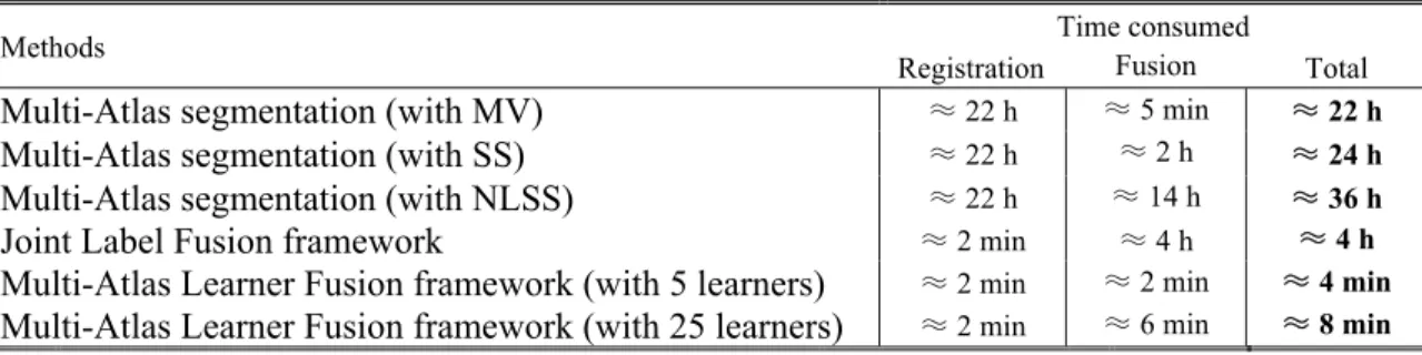
2. Runtime of each method on an Intel Xeon W3550 4 Core CPU (64 bit Ubuntu Linux 12.04) ... 30

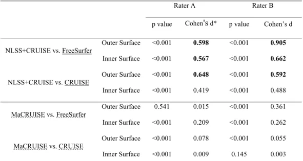
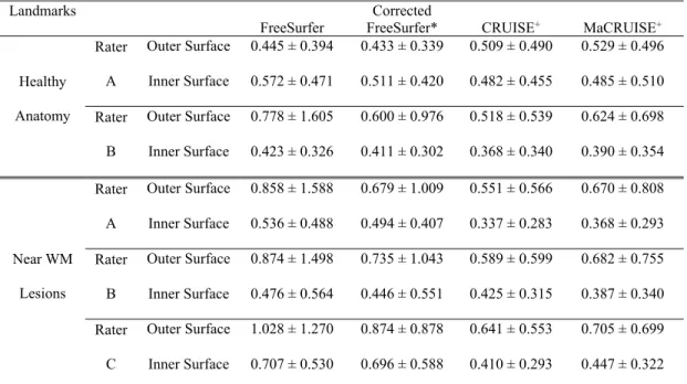
3. Absolute surface errors on subjects with healthy anatomy with MaCRUISE (mean ± standard deviation in mm). ... 52

4. Paired t-test and effect size analyses on absolute surface errors for landmarks with MaCRUISE. ... 52

5. Absolute surface errors with healthy anatomy and WM lesions with MaCRUISE+ (mean ± standard deviation in mm). ... 55

6. Paired t-test and effect size analyses on absolute surface errors for landmarks with healthy anatomy and WM lesions with MaCRUISE+_{... 56}

7. Accuracy test results of TICV ... 100

8. Accuracy test results of PFV ... 101

9. Data summary of 5111 multi-site images. ... 112

10. Quantitative Results of Reproducibility Experiment ... 130

11. Quantitative Results of Robustness Test ... 130

12. Performance of Four Pipelines using All 55 Volumes in A Leave-one-subject-out approach. ... 145

(9)

ix

LIST OF FIGURES

Figure Page 1. The principle of Big Data Medical Image Analysis, which contains (1) large-scale image

processing, and (2) large-scale data analysis. The focus of the dissertation is to provide a Big Data medical image analysis solution, which including large-scale image processing methods, consistent segmentation and surface reconstruction, inter-subject variation control, and large-scale data analysis. Then, we deploy the entire pipeline to understand the lifespan brain aging as an example. ... 2 2. Flowchart demonstrating the multi-atlas learner fusion (MLF) framework. A large collection

of training images is processed offline using a typical multi-atlas segmentation pipeline. The dimensionality of the training images is then reduced, and learners are constructed to map a weak initial estimate to the multi-atlas segmentation. Finally, for a new testing image, the image needs to be projected into the low-dimensional space and the locally appropriate learners can be fused to efficiently and accurately estimate the final segmentation. ... 20 3. Summary of the training data processed through multi-atlas segmentation and their

corresponding representation in the estimated low-dimensional space. The inlays in (A) and (B) illustrate that the PCA distance metric leads to reasonable clustering of anatomical features.

... 21 4. Total variation captured by first N modes from the PCA projection. The upper left figure shows

the total variation captured by first N modes from the PCA. It is got from the percentage of the cumulated sum of the first N eigenvalues among all eigenvalues. The lower left figure shows the derivative of the upper left figure. (b) Coordinate embedding of 3464 training dataset from 6 projects. The first two modes in the PCA low-dimensional space are shown. ... 23 5. Parameter optimization and sensitivity for the number of atlases fused for the initial majority

vote (A), and the type of weak learner used for the AdaBoost classifiers (B). A representative segmentation using the optimized parameters can be seen in (C). Note, on (B), “*” indicates statistically significant difference, and “NS” indicates no significant difference. ... 25 6. Mean accuracy assessment for the defined testing data using the multi-atlas segmentation

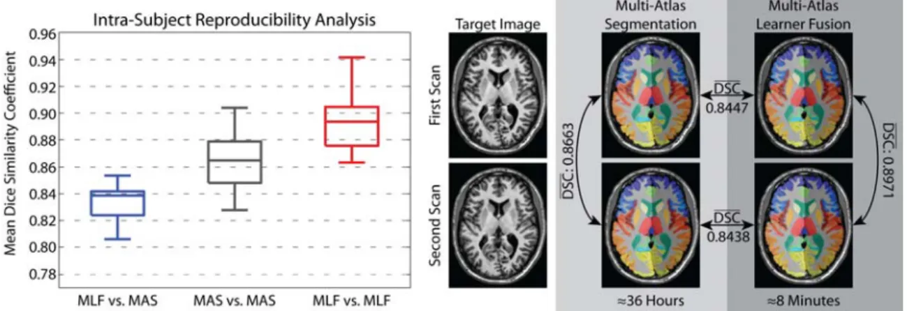
estimate as a “silver standard”. The results demonstrate (1) the MLF framework provides a dramatic decrease in total segmentation time, (2) increasing the number of fused learners has valuable benefits in terms of segmentation accuracy, and (3) fusing more than 5 local learners the MLF framework provides substantial and significant accuracy benefits over the joint label fusion baseline. ... 26 7. Reproducibility analysis on the MMMRR dataset. Note, (1) the MLF similarity to the

multi-atlas segmentation result approaches the intra-subject reproducibility for multi-multi-atlas segmentation, and (2) MLF is significantly more reproducible than multi-atlas segmentation on this dataset. ... 28 8. Summary of the simulation and results. The flowchart shows the framework of the simulation:

(10)

x

registration. (2) 10 of them were used as atlases for multi-atlas segmentation while 80 of them were used as training data for the MLF framework. (3) 3 images were deformed to 27 testing images for comparing the Multi-Atlas segmentation, small-scale model and big data model. The results demonstrate (1) the performance of the MLF framework is significantly improved when using big data model (3464 training images) and (2) the MLF framework under big data model provides the better performance than MV and SS even without using non-local information. ... 30 9. Results of empirical evaluation. The results indicate without using non-local information, the

MLF framework (large-scale) provides better performance than two multi-atlas segmentation algorithms (MV and SS) and has comparable performance as the JLF benchmark. Note that, the multi-atlas segmentation used “non-rigid registration + fusion” framework while the JLF and the MLF used “affine registration + fusion” framework. ... 32 10. Example for one subject, which corresponds to the different methods in Figure II.8. The

anatomical and the manual segmentation of the target image are also provided. ... 33 11. Block diagram of MaCRUISE. Black text indicates the steps in original CRUISE while red text

indicates the additional steps in MaCRUISE. ... 39 12. Results from NLSS multi-atlas segmentation. From the multi-atlas segmentation, we derive

cerebrum segmentation, GM segmentation and WM segmentation. ... 41 13. Here we present the differences and challenges in directly applying multi-atlas hard

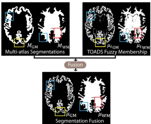
segmentation to cortical reconstruction. (“NLSS+CRUISE”). (a) shows cortical reconstruction based on GM and WM segmentation using CRUISE. (b) shows the consistent surfaces with NLSS multi-atlas. (c) shows that the outer surface (green) and inner surface (magenta) from NLSS+CRUISE are inaccurate on enlarged 2D overlay (red rectangle). The dotted surfaces indicate the improvements by using the proposed MaCRUISE method ... 42 14. Refined segmentations are obtained from segmentation fusion with the following

characteristics: (1) PVE issues in NLSS multi-atlas segmentation are resolved (blue rectangles), (2) the fused segmentations have WM labels consistent with TOADS (red rectangles), and (3) non-cerebrum tissues are cleaned by the multi-atlas segmentation (yellow rectangles). ... 43 15. MaACE compared with the ACE method, (1) MaACE is able to detect sulci in the outer surface

that are not detected by ACE, particularly when CSF evidence is not visible (yellow arrow in b). (2) MaACE also forces sulci locations to be consistent with multi-atlas segmentation at the boundaries of cortical labels (red arrow in b). This figure also shows the enhanced GM membership and skeleton from ACE and MaACE (top row)... 46 16. The CCSE step corrects the inaccurate cortical labels to background or WM, if they are located

outside of the outer surfaces or inside the inner surfaces, respectively. Meanwhile, CCSE adjusts the incorrect volume-wise labels to be cortical labels for voxels between inner and outer surfaces. The distances between voxels and surfaces are provided by the zero set level set functions and . The level of consistency is quantitatively controlled by two consistent coefficients, the inner surface consistent coefficient and the outer surface consistent coefficient . ... 48 17. Inner and outer surfaces are shown for different methods for a healthy subject. The red and

(11)

xi

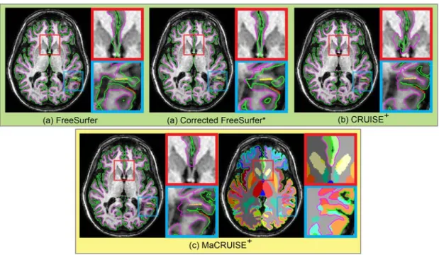
respectively. FreeSurfer and CRUISE are two benchmark methods that achieve accurate surfaces. Note, NLSS+CRUISE does not reconstruct accurate surfaces. Using MaCRUISE, we obtain consistent cortical surfaces and whole brain multi-atlas segmentations. MaCRUISE generates accurate surfaces at lateral ventricles as well as highlighted in yellow rectangles... 51 18. Inner and outer surfaces are shown for each method for an MS subject. Red and yellow dots in

blue and red rectangles are the manual outer and inner surface landmarks, respectively, near WM lesions. Based on the landmarks, CRUISE+ and MaCRUISE+ achieve more accurate surfaces than FreeSurfer and lesion corrected FreeSurfer*. Note that the corrected FreeSurfer* uses the same lesion mask as CRUISE+ and MaCRUISE+, which is generated by Lesion-TOADS. From (c), MaCRUISE+ achieves consistent cortical surfaces and whole brain segmentations that CRUISE+ does not. ... 54 19. This figure shows the sensitivity MaCRUISE has to and by varying them between 0 mm

to 1 mm with 0.05 mm intervals. The upper row shows average Dice improvement from NLSS to CSEE in MaCRUISE. (a) The method has maximum improvement when = . mm and = . mm. (b) The cortical labels follow a similar trend. (c) WM labels are only affected by the inner surface consistent coefficient . (d) The box plot shows the largest Dice improvements of all 132 labels from this dataset ( = . mm, = . mm) compared to the default values in MaCRUISE ( = . mm, = . mm). (e) and (f) demonstrates the improvements of all 98 cortical labels and 2 WM labels respectively. We compare our approaches with the state-of-the-art JLF method as well. “*” indicates statistically significant difference. ... 58 20. This figure shows the average surface distance (ASD) between different methods and the

correlation of lateral ventricle size for the population of elderly subjects. (a) The ASD between MaCRUISE with CRUISE and FreeSurfer is less than 0.5 mm in most cases, but four outliers are found. (b) The size of lateral ventricle is plotted using FreeSurfer and MaCRUISE which identified seven more outliers. A total of 11 inconsistent outliers are detected where failures occured in one of the methods. We note that FreeSurfer systematically estimates smaller ventricle size than MaCRUISE in the outliers. ... 59 21. The four outliers from surface distance analysis are shown. Both whole brain segmentations

and cortical surfaces on axial slices are provided. The areas in red rectangles show the global failures in FreeSurfer whereas MaCRUISE did not exhibit any such failures. ... 60 22. The seven outliers from inconsistent lateral ventricle size are shown. Both whole brain

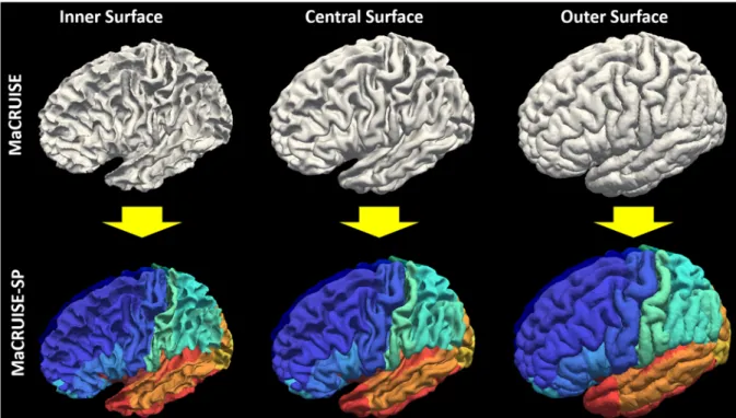
segmentations and cortical surfaces on axial slices are provided. The areas in red rectangles show the global failures while the areas in yellow rectangles show the local inaccurate surfaces. MaCRUISE did not exhibit such failures in any images. ... 61 23. The motivation of MaCRUISEsp was to provide quantitative surface labels for MaCRUISE

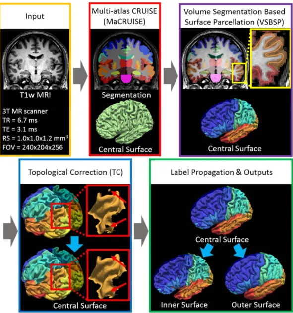
surfaces. ... 66 24. Work flow of MaCRUISEsp. (1) MaCRUISE was deployed on a single T1w MRI volume to

achieve consistent whole brain segmentations and cortical surfaces (inner, central and outer). (2) Surface parcellation was performed on central surface using volume segmentation based surface parcellation (VSBSP). (3) The topological correction is conducted to ensure the one connected component (OCC) for each surface region. (4) The inner and outer surfaces were parcellated on by propagating the labels from central surfaces. Finally, 98 cortical labels were assigned for each surface. ... 68

(12)

xii

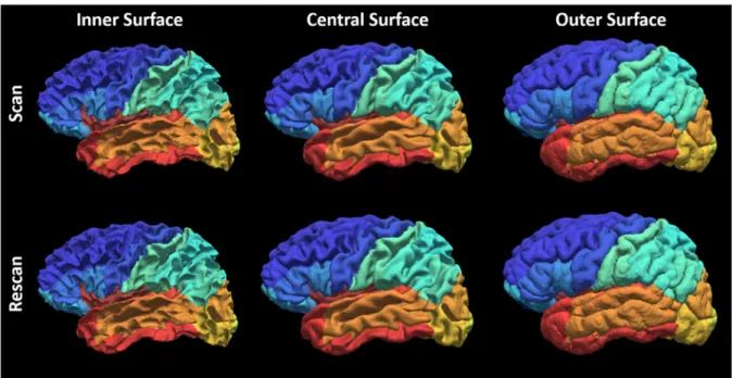
25. Qualitative reproducibility results on the surface parcellation between a randomly selected scan-rescan patient using MaCRUISEsp. ... 70 26. Quantitative segmentations results on the surface parcellation for the entire Kirby21 cohort.

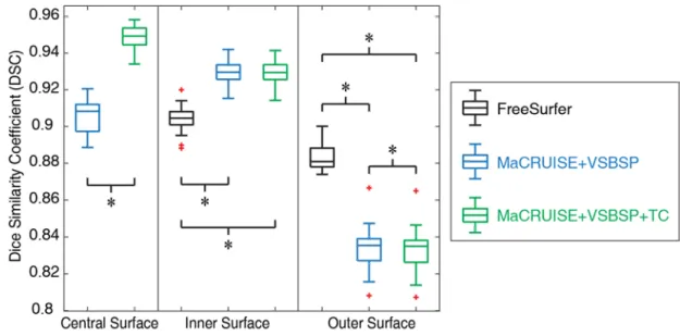
The reproducibility on inner and outer surfaces using FreeSurfer’s Destrieux 2009 atlas (75 labels) were employed as the baseline. The MaCRUISE+VSBSP method as well as the MaCRUISEsp (MaCRUISE+VSBSP+TC) method using BrainCOLOR atlas (98 labels) were presented. The symbol “*” indicated the differences are significant for the Wilcoxon signed rank test for p < 0.01. ... 71 27. The reproducibility of surface metrics (surface area and cortical thickness) were shown. The

Pearson correlation values for four metrics on each label were shown in the left panel. The color of each label corresponds to the Pearson correlation value showed in the color bar. Then, the qualitative results of all labels were shown as the boxplot in the right panel. ... 71 28. Flowchart of training a data-driven dictionary of whole brain probabilistic atlas... 75 29. Flowchart of applying the dictionary to customize a probabilistic atlas for a new subject. ... 77 30. Jensen-Shannon divergence. The comparisons of JS divergence for different atlases are all

significantly different for both withheld and OASIS testing images. ... 79 31. Dice similarity. The comparisons of Dice value for different atlases are all significant for both

withheld and OASIS testing images except the IXI-HH group marked by “Ø”. ... 80 32. One testing subject from OASIS dataset. Top row shows the anatomical image, manual

segmentation, highest probability segmentations using the group probabilistic atlases, Training Set 720 and Training Set 1888. The lower rows show the details of 6 regions. For each region, from left to right are: anatomical image, manual segmentation, probabilistic atlases generated by different methods and their overlays on manual segmentations. ... 81 33. Semi-manual pipeline of establishing atlases. First, the TICV label is obtained by applying a

threshold, morphological operations and the level set method on CT images. Then, the TICV label is propagated to MR image space and the reference PFV label are provided by merging TICV label and the automatic whole brain segmentation. Finally, the semi-manual atlases are obtained by conducting manual refinement on the reference labels. ... 91 34. BC1, BC2 and BC3 atlases are obtained by adding TICV and PFV labels. (a) 20 paired

MR-CT images are used to generate (b) semi-manual atlases. Then the NLSS multi-atlas segmentation is conducted on (c) T1w images 45 OASIS images in BrainCOLOR (BC) atlases to achieve TICV and PFV labels. (d) The first automatic segmentation results are referred as BC1 atlases. (e) Then the original 133 labels from BC are merged with BC1 atlases by keeping the BC labels if conflictions happen. The merged BC2 atlases contain 136 labels including the TICV, PFV and BC labels. (f) The 136 labels are merged back to 4 labels to resolve conflicts and form the BC3 atlases. A subset of BC2 atlases have been made freely available online to facilitate other researchers. We compare the performance of BC1, BC2 and BC3 atlases as well as semi-manual atlases. ... 94 35. Scatter plots comparing FreeSurfer, FSL, SPM12 and NLSS on TICV estimation. In the first

column, different automatic methods are compared with semi-manual segmentations by plotting the TICV volumes with a red line of best fit and NLSS method using semi-manual

(13)

xiii

atlases achieves latest R2_{= 0.970. The remaining columns show the scatter plots between} automatic methods. NLSS method still achieves large R2_{values compared with FreeSurfer,} FSL and SPM12. (b) Box plot of ASIM values between FreeSurfer, SPM12 and NLSS with Semi-manual segmentations. The proposed NLSS (“Ref.”) method achieves significantly higher (“∗”) ASIM scores than FreeSurfer and SPM12. Since FSL only provides scaling factors rather than TICV volumes, it does not have units in (a) and not shown in (b). ... 97 36. Box plots and statistical results on volume accuracy. The statistical analyses were conducted

between the proposed NLSS TICV estimation using semi-manual atlases (marked as reference “Ref.”) with other approaches or different atlases. If the difference was statistically significant, we marked the other method with “*” symbol. Otherwise, we marked it as “N.S.” ... 102 37. Box plots and statistical results on Dice coefficients. The statistical analyses were conducted

between the proposed NLSS TICV estimation using semi-manual atlases (marked as reference “Ref.”) with other approaches or different atlases. If the difference was statistically significant, we marked the other method with “*” symbol. Otherwise, we marked it as “N.S.” ... 103 38. Qualitative results comparing multi-atlas segmentation methods with semi-manual

segmentation. The red contours represent the spatial location of the semi-manual segmentation. The white color indicates the negative error, in which the estimated segmentation is smaller than the semi-manual reference. The green and purple color outside the red contours indicates the positive error, in which the estimated segmentation is larger than reference. ... 104 39. Qualitative results comparing multi-atlas segmentation methods with semi-manual

segmentation. The red contours represent the spatial location of the semi-manual segmentation. The white color indicates the negative error, in which the estimated segmentation is smaller than the semi-manual reference. The green and purple color outside the red contours indicates the positive error, in which the estimated segmentation is larger than reference. ... 105 40. Volumetric reproducibility analysis of different approaches on scan-rescan T1w images. For

all methods, inconsistency of TICV estimation between two scans on the same subject is less than 2%. The statistical analyses were conducted between the proposed NLSS TICV estimation using semi-manual atlases (marked as reference “Ref.”) with other approaches or different atlases. If the difference was statistically significant, we marked the other method with “*” symbol. Otherwise, we marked it as “N.S.” ... 106 41. Sensitivity to NLSS non-local search parameters. ... 108 42. The large-scale cross-sectional framework on 5111 multi-site MR 3D images. ... 113 43. Volumetry and growth rate. The left plot in (a) shows the volumetric trajectory of whole brain

volume (WBV) using C-RCS regression on 5111 MR images. The right figure in (a) indicates the growth rate curve, which shows volumetric change per year of the volumetric trajectory. In (b), C-RCS regression is deployed on the same dataset by additionally regressing out TICV. Our growth rate curves are compared with 40 previous longitudinal studies [1] on smaller cohorts (21 studies in (a) without regressing out TICV and 19 studies in (b) regressing out TICV). The standard deviations of previous studies are provided as black bars (if available). The 95% CIs in all plots are calculated from 10,000 bootstrap samples ... 117 44. Lifespan trajectories of 15 NOIs are provided with 95% CI from 10,000 bootstrap samples. The

(14)

xiv

trajectories with CI using C-RCS regression method by regressing out gender, field strength and TICV (same model as Figure VII.2b). For each NOI, the piecewise CIs of six age bins are shown in different colors. The piecewise volumetric trajectories and CIs are separated by 7 knots in the lifespan C-RCS regression rather than conducting independent fittings. The volumetric trajectories on both sides of each NOI are derived separately except for CB. ... 118 45. The six structural covariance networks (SCNs) dendrograms using hierarchical clustering

analysis (HCA) indicate which NOIs develop together during different developmental periods (age bins). The distance on the x-axis is in log scale, which equals to one minus Pearson’s correlation between two curves. The correlation between NOIs becomes stronger from right to left on the x-axis. The horizontal range of each colored rectangles indicates the 95% CI of distance from 10,000 bootstrap samples. Note that the colors are chosen for visualization purposes without quantitative meanings. ... 119 46. An example of the inconsistency of 3D joint label fusion (JLF) segmentation across

longitudinal multiple scans from the same subject. The 4DJLF is proposed to improve the consistency while maintain the sensitivity. ... 123 47. The 4DJLF framework. First, the same set of atlases are registered to the longitudinal target

images (3 time points in figure). Then, the matrices are calculated using Eq. 8.13. Finally, the spatial temporal performance of all atlases are model by Eq. 8.14, which leads to the final segmentations (“Seg.”). Note that the upper right × matrix is identical to Eq. 8.15. The original JLF estimates the block diagonal elements of the generalized covariance matrix (highlighted in magenta, green, and yellow) which would result in independent temporal estimates. ... 125 48. Quantitative results. (a) The reproducibility experiment shown that the proposed 4DJLF had

overall significantly better reproducibility than JLF and JLF-Multi. (b) The robustness test indicated that 4DJLF maintained the sensitivity as JLF, while JLF-Multi was not able to do so. The red “*” means the method satisfied both p<0.01 and effect size>0.1 compared with JLF (“Reference”), while the “N.S.” means at least one was not satisfied. The black “*” means the difference between two methods satisfied both p<0.01 and effect size>0.1. ... 129 49. This figure demonstrated the longitudinal changes of whole brain volume, gray matter volume,

white matter volume and ventricle volume for all 6 subjects (21 time points). The black arrows indicated that the proposed 4DJLF reconciles some obvious temporal inconsistency by simultaneously considering all available longitudinal images. ... 131 50. Qualitative results of deploying longitudinal segmentation methods on two examples. ... 132 51. (a) presents heterogeneous sequences in clinical acquired abdominal MRI as well as the

examples of splenomegaly spleens on MRI. (b) shows the spleen size and sequence type of all 55 MRI. ... 135 52. Multi-atlas labeling steps for each of the four pipelines. Pipeline 1 conducted multi-atlas label

fusion (MLF) on all registered atlases without using atlas selection. Pipeline 2 employed the SIMPLE atlas selection method before performing MLF. Pipeline 3 used the craniocaudal spleen length (L) to guide the atlas selection. Pipeline 4 evaluated the proposed L-SIMPLE method, which integrated the feature L to the SIMPLE atlas selection under the Bayesian framework. For all pipelines, a post refinement procedure was included to ensure the topological correctness of the spleen segmentation (one connected component). ... 137

(15)

xv

53. This figure presents an example of using different atlas selection strategies. The upper panel reflects the registration results of registering each atlas to the target image. The target image is shown as the left figure on the lower panel. The registered atlases are arranged based on the Dice similarity coefficient (DSC) to the target manual segmentation, whose DSC increased from top left to bottom right. Pipeline 1 (in blue rectangles) employed all registered atlases in the label fusion. Pipeline 2 (in pink rectangles) performed the atlas selection using SIMPLE method. Pipeline 3 (in green rectangles) used the craniocaudal spleen length (L) to guide the atlas selection. Pipeline 4 (in yellow rectangles) integrated L and SIMPLE to the proposed L-SIMPLE method under the Bayesian framework. In this example, Pipeline 4 chose the better atlas candidates (lower rows in upper panel) for the atlas selection, which achieved the highest DSC relative to the manual segmentation. ... 138 54. The scatter plot demonstrated that 2890 registrations have been performed on all possible

combinations between 55 clinical acquired splenomegaly images. The coordinate of each dot corresponded to the craniocaudal spleen length (L) of the source and target scan of the registration. The color of each dot indicated the DSC value between the registered spleen label and the manual segmentation. ... 143 55. The qualitative results of four pipelines on the three subjects with largest, median and smallest

DSC of Pipeline 4 with GC were shown with manual segmentation. For each pipeline, the “no GC” indicated the results without Graph Cuts while the “with GC” demonstrated the results with Graph Cuts. ... 144 56. The quantitative results of four pipelines on Dice similarity coefficient (DSC), mean surface

distance (MSD) as well as Hausdorff distance (HD) are shown in boxplots. The “no GC” indicated the results without Graph Cuts while the “w. GC” demonstrated the results with Graph Cuts. The statistical analyses were conducted between the proposed Pipeline 4 L-SIMPLE with Graph Cuts method (marked as reference “Ref.”) with other approaches. Statistically significant, differences are marked with a “*” symbol. Non-significant differences are indicated with “N.S.” ... 144 57. The correlation analyses between different pipelines with manual segmentation. The

semi-automated pipelines achieved higher Pearson correlation values than fully-semi-automated pipelines and fully-manual L measurements. The “+” and “=” indicated that the Pipeline 3 and 4 integrated the information derived from Pipeline 1 and 2 plus the craniocaudal spleen length (L). The “corr.” reflected the Pearson correlation values. The “no GC” indicated the results without Graph Cuts while the “with GC” demonstrated the results with Graph Cuts... 146 58. The sensistivty analyses of the proposed L-SIMPLE method on multi-contrast images. (a)

demonstrates that using both T1w and T2w images as atlases achieved better performance than only using T1w or T2w atlases on segmenting T1w images. (b) shows that using both T1w and T2w images as atlases achieved better performance than only using T1w or T2w atlases. From (a) and (b), it is evident that the performance of using the same sequence on both atlases and targets did not yield a significant difference on DSC compared with using the different sequences for atlases and targets respectively. The “*” symbol indicates significant differences. ... 147 59. The proposed network structure of the Splenomegaly Segmentation Net (SSNet). The number

of channels of each encoder is shown in the green boxes, while the number of channels of each decoder is two. The image (or feature map) resolution for each level is shown on the left side of this figure. ... 151

(16)

xvi

60. The testing accuracy of different epochs was shown in this figure. The y axial indicated the mean Dice similarity coefficients (DSC) on all testing volumes, while the x axial presented the epoch number from one to ten. The dashed curves were the testing accuracy for the case that only axial images were used as training and testing images. The solid curves were the testing accuracy for the case that all axial, coronal and sagittal view images were used in both training and testing scenario. ... 154 61. The qualitative results of different methods. The segmentation results of Unet, GCN and SSNet

on using (1) only axial 2D images, and (2) all axial, coronal and sagittal 2D images are shown in the figure for different columns. The manual segmentation results for the same subjects are presented as well. The results of three subjects were selected from the highest, median and lowest DSC from the SSNet’s testing data. ... 155 62. The quantitative results of different methods. The box plots in left panel indicate the results of

using only axial view images, while the right panel presents the results of using all axial, coronal and sagittal images as in both training and testing. The Wilcoxon signed rank tests were employed as statistical analyses, where “Ref.” indicates the reference method. The “*” indicates the p<0.01 while the “NS” means not significant. ... 156 63. The upper row shown that carnonical methods trained by normal spleen failed in splenomegaly

segmentation. The lower row shown that the proposed EssNet achieved splenomegaly segmentation from unpaired MRI and CT training images without using CT labels. ... 160 64. The left side was the CycleGAN synthesis subnet, where A was MRI and B was CT. G_1 and

G_2 were the generators while D_1 and D_2 were discriminators. The right subnet was the segmentation subnet for an end-to-end training. Loss function were added to optimize the EssNet. ... 161 65. The qualitative results of the synthesized images and segmentations in training Path A and Path

B. ... 162 66. The qualitative results of (1) three canonical methods using CT manual labels in CT

segmentation, and (2) CycleGAN+Seg. and the proposed EssNet methods without using CT manual labels. The splenomegaly CT labels were only used in validation and excluded from training for (2). Moreover, later methods not only performed spleen segmentation but also estimated labels for other organs, which were not provided by canonical methods when such labels were not available on CT. ... 164 67. The boxplot results of all CT splenomegaly testing images, where “*” means the difference are

significant at p<0.05, while “N.S.” means not significant. ... 165 68. Top: Non-contrast CT with cropped images of the kidney in which pyelocalyceal system is not

visualized. Bottom: Excretory phase of CT Urogram with cropped images of kidney and

pye-localyceal anatomy illuminated during excretion of contrast by the kidneys. ... 168 69. The workflow of the proposed framework. First, the whole kidney was localized and

segment-ed using multi-atlas segmentation. Then the pyelocalyceal structure was segmentsegment-ed from a Gaussian Matured Model and the tree structure was subsequently derived. Key landmarks (yellow dots) were manually identified from the 3D reconstruction and tree structure to

(17)

xvii

70. Quantitative results of the segmentation and angle measurements for a single kidney. Top row: 3D reconstruction of the kidney, 3D reconstruction of the pyelocalyceal structure, tree struc-ture. Bottom row: Overlays of reconstructions and tree structure, traditional 2D measurement [1] of IPA (red lines) using averaged 2D image (blue lines indicate key landmarks), and the 3D IPA measurement (red lines) using described method. ... 171

(18)

1

Chapter I.

Introduction

1.

Overview

Medical imaging refers to the technologies of creating visual representation of the interior of human body for scientific research and clinical analysis. Different imaging technologies (modalities) provide different properties, which enables us to investigate human body using particular field of view (FOV) and image contrast [2]. The history of medical imaging can be traced back to the discovery of X-ray in 1895 by Wilhelm Conrad Roentgen, who took the first X-ray on his wife’s hand [3]. Since then, many milestones have been made to enable new modalities and devices that we are performing currently (e.g., Ultrasound, Computed Tomography (CT), Magnetic Resonance Imaging (MRI), etc.) [2].

Two-dimensional (2D) or three-dimensional (3D) medical images are the major outcomes from medical imaging techniques. Based on such images, clinical practitioners can make diagnoses by visually investigating the medical images, which relies heavily on the experts’ experiences. To provide more information for clinical diagnoses and enable the scientific research, quantitative metrics are extracted from the qualitative images, which results in the research field called medical image analysis (MIA) [4]. To derive quantitative information from medical images, the expert manual delineation has been regarded as the “gold standard” due to the high reliability [5]. However, the manual delineation is resource and time consuming even with the advanced image-guided interactive tools [6]. Therefore, the fully-automated medical image processing is appealing for extracting quantitative metrics from qualitative medical images. Medical image analysis is an interdisciplinary field of engineering, computer vision, mathematics, data science and medicine, which focuses on the computational analysis of the acquired medical image rather than image acquisition (medical imaging) [4]. The computational methods in MIA can be categorized to two parts (Figure I.1). The first part is the image processing (Figure I.1a), which uses mathematical and computational models to extract quantitative information or metrics from medical images. Representative image processing approaches are preprocessing [7], registration [8], segmentation [5], surface reconstruction [9], etc. The second part is called data analyses (Figure I.1b), which investigates and

(19)

2

understands the hidden regularities behind the metrics extracted by image processing. The common data analyses approaches include statistical analysis [10], visualization [11], modality specific computing [7], etc.

Historically, the medical image analysis on structural images was limited to a small-scale cohort (e.g., <500 images), whose images were collected from a single scanner (site) (e.g., [12-23]). The rationales of using a small cohort are that (1) it is difficult for a single lab to collect a large-scale cohort (e.g., >5000 images) considering the time and resource consumption. (2) There are the difficulties in data sharing and collaborations between different institutes (e.g., need for approval from institutional review board (IRB)). (3) The image quality and homogeneity are easier to control by using small-scale image cohort collected from a single scanner.

In the past decade, advancements in data sharing and robust processing have made available considerable quantities of brain images all over the world, which has been changing the way of performing medical image analysis to the Big Data (large-scale) fashion [23, 24]. The recent special issue of 20th

Figure I.1. The principle of Big Data Medical Image Analysis, which contains (1) large-scale image processing, and (2) large-scale data analysis. The focus of the dissertation is to provide a Big Data medical image analysis solution, which including large-scale image processing methods, consistent segmentation and surface reconstruction, inter-subject variation control, and large-scale data analysis. Then, we deploy the entire pipeline to understand the lifespan brain aging as an example.

(20)

3

anniversary of the Medical Image Analysis journal (MedIA) demonstrates this challenge and opportunity in the first paragraph of “Future Directions” chapter “Big data is becoming a reality with very large scale imaging projects underway or planned. This new scale of data is enabling the solution of challenging problems where the simplicity of methods can offset by the quantity of data available. There are very exciting opportunities at the interface of MIA and the field of Medical Informatics; however there a very few people currently working in both areas.”[25].

The large-scale medical images are typically collected from multiple sites, which leads to the greater inter-subject variations than traditional small-scale cohorts. For instance, it is important to rectify the inter-subject variations in acquisitions, scanning protocols, scanner differences, population variations etc. in Big Data image analysis. Existing efforts on reconciling such variations are to (1) standardize the format and of data sharing[26], (2) perform meta-analysis using more data [27-29], (3) propose advances in image processing algorithms [30, 31]. However, given the fact that “The development of large-scale medical image analysis algorithms has lagged greatly behind the increasing quality (and complexity) of medical images and the imaging modalities themselves” [23], there is an urgent demand to develop large-scale image processing frameworks for the robust and timely medical image analysis [23].

Herein, new image processing methods and data mining approaches, compatible for the large-scale scenario, are required to (1) reduce the computational time for large-scale image processing, (2) achieve robust and consistent volume and surface metrics, (3) reconcile inter-subject variations for large cohorts, (4) perform large-scale data analysis using the metrics derived from image processing, and (5) to be robust for variations on intensities and contrasts for multi-site scans.

Beside the methodological challenges, applying large-scale medical image analysis techniques on investigating clinical and research problems leaves many rooms for researchers to fill in. Recent works have demonstrated the advantage of conducting large-scale medical image analysis in understanding prevalent human disorders [32], brain connectivity [33], psychiatric disorder [34] etc. Yet, only limited works have been conducted on investigating lifespan human brain aging, an essential topic in neurological research and clinical investigation, using Big Data medical images. Historically, age-related changes have

(21)

4

been studied in detail for specific age ranges (e.g., early childhood, teen, young adults, elderly, etc.) or more sparsely sampled for wider considerations of lifetime. Contemporaneous advancements [23, 24] in data sharing have made considerable quantities of brain images available from normal, healthy populations, which enable availability of the Big Data for investigating lifespan human aging.

Another interesting application of performing large-scale image processing methods is to explore the anatomies of abdomen organs. For instance, accurate non-invasive spleen volumetric size estimation plays an essential role in splenomegaly diagnosis and scientific studies [35]. Ultrasound [36-38] and computerized tomography (CT) [39-41] have been widely used in the spleen segmentation, yet, limited studies have been applied to magnetic resonance imaging (MRI) [42-44]. A major challenge of automated MRI spleen segmentation is that the absolute intensity of MRI is not in a quantitative scale like the Hounsfield Units (HU) in CT. Another challenge is that the relative intensity contrasts of abdominal tissues are in large variation using the different contrast mechanisms (e.g., T1-weighted (T1w), T2-weighted (T2w), proton density (PD), etc.). Such challenges hinder frequently used CT segmentation methods, which depend on absolute intensity scales, to be applied on the large-scale MR cohorts directly. Another direction is to model pyelocalyceal anatomy for the kidney, which can also influence the success rate of various treatment modalities of kidney stone. The traditional methods of deriving such quantitative measurements have relied on 2-dimensional images of a 3-dimensional system as well as manual delineations, which are both cumbersome and potentially inaccurate during treatment planning.

Herein, we present several new methods to address key technical challenges in large-scale medical image analyses and integrated such methods to investigate lifespan brain aging and abdominal image evaluation.

2.

Challenges in Large-scale Image Analysis

The increasing demands of imaging-based diagnosis and rapid developments of the advanced medical imaging techniques lead to the rapid growth of imaging data produced by hospitals and institutes [23]. Only in the past decade, the worldwide clinical and scientific collaboration has provided hundreds of

(22)

5

terabytes of data, which has been made publicly available [24]. The dramatic increasing in the volume and dimension of the medical images results in the challenges of image storage, processing and analysis [23, 24]. However, new clinical and scientific opportunities are arising to explore the valuable information from the large-scale data [23, 24]. Ideally, the automated medical image analysis algorithms are the key to extract biomarkers (biometrics) efficiently and robustly [23, 24]. However, since traditional medical image analysis techniques historically designed for smaller cohorts, new challenges emerge when deploying the existing methods under large-scale scenarios [23-25]. This situation leads to the high demands of novel medical imaging processing and data analyses algorithms, which are able to deal with the unprecedented large-scale datasets [23-25].

2.1.Large-scale Brain Image Processing

Image segmentation and surface reconstruction are two essential methods in large-scale brain image processing. Image segmentation is a computational procedure that assign a distinct label for every voxel in the digital medical images [5]. The representative image segmentation approaches include, but not limit to, threshold based segmentation [45], C-means clustering [46], deformable models [47], graph cuts [48], shape model [49], appearance model [50], learning based model [51], atlas-based segmentation [52-54] etc. Using image segmentation, we are able to derive volume based metrics (e.g., volume size, shape, momentum etc.) of each ROI. Surface reconstruction is another fundamental image processing approach, whose aim is to reconstruct the surfaces of different ROIs based on segmentation and deformable model. The typical surface reconstruction tools include, FreeSurfer [55], CRUISE [56], BrainVISA [57] etc. From the surface reconstruction, the surface based metrics (e.g., surface area, thickness, curvature etc.) are derived.

In large-scale image processing, we not only want to achieve the higher sensitivity from each individual subject compared with traditional image processing, but also want to achieve higher robustness of segmentation and surface reconstruction across the large-cohort. Historically, the image segmentation and cortical reconstruction are typically conducted independently, which may lead to inconsistent metrics

(23)

6

from two procedures. Such spatial inconsistences can hinder the simultaneous usages of volume and surface features in large-scale data analyses. There are limited reports of methods [58-60] for consistent whole brain volumetric segmentation and cortical surface reconstruction.

Another challenge in large-scale medical image analysis is the large inter-subject variations. Unlike the traditional small-scale image analysis, whose variations are typically well controlled by an individual institute. Larger inter-subject variations need to be controlled, at least alleviated, in the large-scale scenarios. To control the inter-subject variations, the total intracranial volume (TICV) has been widely used as a covariate in brain volumetric analyses [61-67]. Compared with whole brain volume (WBV) [68], TICV is often preferred since it provides an estimation of premorbid brain size [69, 70]. Historically, the existing methods performed TICV estimation only used a single affine registration. To reconcile the large inter-subject variability, Commowick et al. proposed to build a personal specific anatomical atlas for head and neck [71]. However, this framework cannot be directly applied to establish probabilistic atlases since each probabilistic atlas is averaged from a group of segmentations.

2.2.Large-scale Image Analysis

Image processing provides large-scale measurements/features (e.g., volume, surface, TICV) from big medical image cohorts [72]. Then data analysis used such measurements to explore the hidden regularities behind the images, which is related to data mining [23-25, 73]. The next challenge is to explore the large-scale metrics by either developing new or adapting existing computational and statistical models. However, traditional image analysis methods can yield less optimal performance for the large-scale challenge. Taking the lifespan brain volume trajectory as an example, prevalent analysis approaches have had difficulties addressing (1) complex volumetric developments on the large cohort across the life time (e.g., beyond cubic age trends), (2) accounting for confound effects, and (3) maintaining an analysis framework consistent with the general linear model (GLM) approach pervasive in neuroscience.

2.3.Computational Efficiency

(24)

7

issues such as higher demands on computational resources and time. To alleviate the computational complexities, learning based algorithms have been successfully employed to speed up the labeling process including, but not limited to, SVMs [74-76], random forest[77, 78], artificial neural networks [74, 79], logistic LASSO [80] and boosting [75]. Unfortunately, the previous learning-based schemes are mostly limited to single anatomical region segmentation rather than whole brain. When applied on whole brain, the computational expensive non-rigid registration is typically required to alleviate large inter-subject variation.

2.4.Large-variations for the Abdomen

The last challenge is that most of the prevalent medical image analysis approaches are historically designed for neuro images, which hinders us to apply such methods (e.g., preprocessing, registration, multi-atlas label fusion) to abdomen directly [81]. A major reason is that the abdomen has greater heterogeneity than the brain. Moreover, the locations of abdominal viscera for same subject can change obviously between two scans. For inter-subject variations, the heterogeneity is even greater. For instance, the spleen size of splenomegaly cohort varies from 368 cubic centimeter (cc) to 5670 cc reported by [82].

3.

Context for Advancing Large-scale Image Processing

Hundreds of secondarily derived biomarkers and biometrics can be extracted from a single medical image using advanced medical image processing methods, which allows the researchers to explore the hidden spatial and temporal relationships from large-scale dataset. We first introduce the multi-atlas segmentation (MAS) theory, then present two new techniques based on multi-atlas principle: (1) large-scale multi-atlas learner fusion (reduces the computational time), and (2) consistent multi-atlas segmentation and surface reconstruction (provides consistent volume and surface). Then, to reconcile the inter-subject variations, the data-driven probabilistic atlas and total intracranial volume estimation methods are introduced.

(25)

8

3.1.Multi-atlas Segmentation

Among segmentation methods, atlas-based segmentation is one of the most prominent families, which uses a pairing of structural MR scans and corresponding manual segmentation. In atlas-based segmentation models, an existing dataset (atlas) is spatially transferred to a previously unseen target image through deformable registration. Single-atlas segmentation has been successfully applied to some applications [83-85]. Yet, more recent approaches employ a multi-atlas paradigm as the de facto standard atlas-based segmentation framework [86, 87]. In multi-atlas segmentation, the typical framework is: (1) a set of labeled atlases are non-rigidly registered to a target image [8, 88-90], and (2) the resulting label conflicts are resolved using label fusion [87, 91-99].

The most prevalent multi-atlas label fusing theory has been developed to model the spatial relationships between atlases and targets in 3D scenarios. To improve the performance of 4D MAS for longitudinal data, we propose a novel longitudinal label fusion theory, called 4D joint label fusion (4DJLF) to incorporate the probabilistic model of temporal performance of atlases to the voting-based fusion.

3.2.Multi-atlas Learner Fusion

One major concern of applying multi-atlas segmentation framework on Big Data is the computational complexity as it typically takes over 24 hours for more than ten non-rigid registrations and the following multi-atlas label fusion. To decrease overall computational complexity, new approaches have emerged to minimize registration time. One of the most common methods is the atlas selection [97, 100-102], which reduces the times of registration by keeping the most representative atlases. Another direction is to use the learning based scheme, which grasps the non-local correspondences offline [91-93, 103, 104]. Advanced by the large-scale images, we present multi-atlas learner fusion (MLF), a framework for replicating the robust and accurate multi-atlas segmentation model, while dramatically lessening the computational burden.

3.3.Consistent Multi-atlas Volume and Surface Computing

(26)

9

independent processing in neuroimaging [105-110]. As a result, such spatial inconsistences can further hinder the consistent brain morphometry analyses. There are limited reports of methods for consistent whole brain volumetric segmentation and cortical surface reconstruction [58-60, 106, 111]. In this dissertation, we presented the multi-atlas CRUISE (MaCRUISE) method to achieve consistent whole brain segmentation and cortical surface reconstruction.

3.4.Big Data Driven Probabilistic Atlas

Probabilistic atlases are essential in understanding the spatial variation of brain anatomy, in visualization, and data processing. However, inter-subject variability is normally greater than inter-group variability, which hinders group-based atlases to capture individual variation. Advanced by large-scale training images, we presented a large-scale data-driven framework to learn a dictionary of the whole brain probabilistic atlases (132 regions) from 1888 heterogeneous 3D MRI training images.

3.5.Total Intracranial Volume Estimation

TICV is a widely used metric to reconcile inter-subject variations in neuro imaging, which is estimated by the volume inside the brain cranium including gray matter (GM), white matter (WM), cerebrospinal fluid (CSF) and meninges [112]. To derive accurate TICV estimation from brain MRI scan, a number of approaches have been developed and evaluated [113-122] [106] [117]. However, none of them estimate TICV by counting the voxels inside skull, which is a natural way of calculating TICV. In this dissertation, we present a multi-atlas based TICV estimation method using Non-Local Spatial STAPLE (NLSS) which is more accurate than previous methods and consistent with whole brain multi-atlas segmentation.

4.

Large-scale Data Analysis

The large-scale data analysis has been broadly applied to medical research and healthcare in past decades, which enables us to establish the correlations between qualitative data (e.g., demographic data), quantitative medical records (e.g., laboratory values) [123], and diseases [124]. Different from the medical

(27)

10

records, the large-scale image data analysis has not been widely investigated due the high degree of freedom in big image cohorts.

4.1.Large-scale Multi-site Cohorts

The maturation of medical imaging technologies as well as the image sharing and storage approaches provide the opportunity to deploy large-scale analysis on medical images. Investigating fundamental diseases using multi-scale images [125], as well as multi-site images [126] have been recognized during the past decade. The National Institutes of Health (NIH) National Database of Autism Research (NDAR) ([127], https://ndar.nih.gov/) is a database of understanding the autism disease. The National Institute on Aging's (NIA) Baltimore Longitudinal Study of Aging (BLSA) ([128, 129], https://www.blsa.nih.gov/) is a clinical research programs of understanding aging and aging-related diseases. The collections of functional MRI (fMRI) have been publicly available on both task-based fMRI from OpenfMRI project ([130], https://openfmri.org/) and resting-state fMRI from “1000 Functional Connectomes” project (fcon_1000) ([131], http://fcon_1000.projects.nitrc.org/). Other publicly available cohorts include Information eXtraction from Images (IXI), Open Access Series on Imaging Studies (OASIS) [132] and Multi-Modal MRI Reproducibility Resource (MMMRR)[133].

4.2.Large Inter-subject Variation

For a single study, the medical imaging data may not face the difficulties using existing processing algorithms and statistical method. However, as data sets from different studies, populations and sites are amassed into a large-scale cohort, considerable challenges emerge. For instance, it is challenging of rectifying the inter-subject variations in acquisitions, scanning protocols, scanner differences, population variations etc. Recent efforts on reconciling such variations are to (1) standardize the format and of data sharing[26], (2) perform meta-analysis using more data [27-29], (3) propose advances processing algorithms [30, 31]. However, if any, common solutions are well accepted to perform image analysis by rectifying such variations on large-scale image cohorts [24].

(28)

11

4.3.Lifespan Brain Aging

In the past decade, many efforts have been made of performing Big Data medical image analysis in understanding, but not limited to, Parkinson’s disease [32], brain connectivity [33], psychiatric disorder [34]. However, few, if any, works have been done on investigating the lifespan aging, the development of brain structures across lifespan, which is a key topic in understanding neuro-development. Herein, investigating lifespan aging on human brain is an appealing application of integrating the new Big Data medical image processing and analysis approaches. In this dissertation, we propose to investigate the lifespan human brain aging on more than 5,000 MR structural images.

5.

Robust Multi-model Abdomen Image Processing

5.1.Atlas-based Splenomegaly Segmentation

Splenomegaly is an abnormal enlargement of the spleen, which is associated with liver disease, infection and cancer [134]. Accurate non-invasive spleen volumetric size estimation plays an essential role in splenomegaly diagnosis and scientific studies [35]. Spleen segmentation using Ultrasound [36-38] and computerized tomography (CT) [39-41] have been used as the major imaging techniques in quantifying spleen size [135, 136]. However, the MRI has not been widely used as the absolute intensity of MRI is not in a quantitative scale like the Hounsfield Units (HU) in CT. Another challenge is that the relative intensity contrasts of abdominal tissues are in large variation using the different contrast mechanisms (e.g., T1-weighted (T1w), T2-T1-weighted (T2w), proton density (PD), etc.). In this dissertation, we propose to use atlas segmentation framework with Bayesian atlas selection and surface constraint on robust multi-contrast MRI spleen segmentation for splenomegaly.

5.2.Deep Learning Based Splenomegaly Segmentation

In recent years, deep learning methods have shown their superior performance on automatic spleen segmentation compared with traditional methods [137]. However, the existing deep learning methods are typically deployed on CT images with normal size spleen (e.g., spleen size < 500 cubic centimeter (cc)).

(29)

12

When dealing with splenomegaly MRI segmentation (e.g., spleen size > 500 cc), we need to deal with large inhomogeneity on intensities of clinical acquired MR and large variations on shape and size of spleen for splenomegaly patients [138]. Recently, global convolutional network (GCN) have shown advantages in sematic segmentation on natural images with large variations by using larger convolutional kernels [139]. Meanwhile, adversarial networks have been proven able to refine the semantic segmentation results [140]. In this dissertation, we propose a new Splenomegaly Segmentation Network (SSNet) to perform the splenomegaly MRI segmentation under the image-to-image framework with the end-to-end training. In SSNet, the GCN is used as the generator while the conditional adversarial network (cGAN) is employed as the discriminator [18].

One major limitation of DCNN methods is that we typically have to manually trace a new set of training data when segmenting new organs or new imaging modalities. For instance, a DCNN trained with normal spleens was not able to capture spatial variations of splenomegaly. Image synthesis has been used to segment images for one modality from another [141-144], yet, paired images were typically required for traditional methods. Recently, two stage methods have been proposed to use cycle generative adversarial networks (CycleGAN) [145] to synthesize training images for a target modality[146, 147]. Then, these efforts trained a segmentation network independently using synthetic images [148]. However, these two independent stages did not use the complementary information between synthesis and segmentation. Herein, we proposed a novel end-to-end synthesis and segmentation network (EssNet) to achieve the unpaired MRI to CT image synthesis and CT splenomegaly segmentation simultaneously without using manual labels on CT.

5.3.Characterization of Pyelocalyceal Anatomy for Kidney

Nephrolithiasis is a costly and prevalent disease that is associated with significant morbidity including pain, infection, and kidney injury. While surgical treatment of kidney stones is generally based on size and quality of the stones, studies have suggested that specific characteristics of pyelocaliceal anatomy, such as the lower pole infundibulopelvic angle, can also influence the success rate of various

(30)

13

treatment modalities [3, 4]. However, the traditional methods of deriving such quantitative measurements have relied on 2-dimensional images of a 3-dimensional system as well as manual delineations, which are both cumbersome and potentially inaccurate during treatment planning [3, 5, 6]. In this dissertation, we propose a novel non-invasive framework that automatically achieves a tree structure of the renal collecting system using CT urograms, allowing for 3-dimensional characterization of the pyelocaliceal anatomy.

6.

Contributions

The primary contributions are as follows. In Chapter II we present an efficient whole brain segmentation approach by learning features from large-scale MRI data. In Chapter III we present a novel multi-atlas CRUISE (MaCRUISE) method to combine the multi-atlas whole brain segmentation with brain cortical surface reconstruction. In Chapter IV we present a surface parcellation method to parcellate reconstructed whole brain surfaces to detailed cortical labels. Chapter V presents a novel data-driven method to establish a target image specified probabilistic atlas from large-scale cohorts. Chapter VI presents a novel simultaneous total intracranial volume (TICV) and posterior fossa volume (PFV) segmentation algorithm to achieve better performance than baseline methods. Chapter VII explore the life-span brain volume trajectories on whole brain, network, and region levels on more than 5,000 multi-site MRI brain volumes. The volumetric features were obtained using multi-atlas segmentation and a novel covariate-adjusted restricted cubic spline regression method was proposed to model the non-linear trajectory curves. In Chapter VIII we extend the multi-atlas label theory from 3D to 4D by considering the spatial temporal performance of registered atlases for longitudinal scenario. In Chapter IX we present a novel atlas-selection based segmentation method to perform MRI splenomegaly segmentation. We further leverage the splenomegaly segmentation accuracy by combing deep convolutional neural network and adversarial network in Chapter X. Chapter XI present a synthesis learning based segmentation method to perform splenomegaly segmentation on CT without having CT ground truth. In Chapter XII, we revisit the pyelocalyceal anatomy in management of kidney stone using 3D segmentation methods. Finally, we conclude in Chapter XIII by summarizing contributions and possible future directions.

(31)

14

6.1. Contributions on Brain

• We proposed the MLF framework cuts the runtime on a modern computer from 36 hours down to 3-8 minutes, which accelerate the multi-atlas segmentation on large-scale image. It explores the possibilities and limitations of designing fast whole brain segmentation methods on large-scale training images.

• We designed and implemented MaCRUISE to achieve consistent whole brain segmentation and cortical surfaces. Using MaCRUISE, we achieve 132 volume labels and 98 surface labels from a single T1-weighted (T1w) MRI scan by integrating previous separated multi-atlas segmentation theory and surface reconstruction theory.

• We present a data-driven framework to build a personal specific probabilistic atlas under the large-scale data scheme.

• We proposed a robust TICV estimation method using multi-atlas label fusion, which has been shown to be more accurate than previous methods. We created a set of TICV brain atlases to be publicly available for our community.

• We proposed to use C-RCS regression method within a multi-site cross-sectional framework and revisit the brain volumetry problem using more than 5,000 MR images.

• We proposed 4DJLF under the general label fusion framework by simultaneously incorporating the spatial and temporal covariance on all longitudinal time points, which is a longitudinal generalization of a leading joint label fusion method (JLF) that has proven adaptable to a wide variety of applications.

6.2. Contributions on Abdomen

• We performed the first study on model MRI splenomegaly segmentation with multi-atlas segmentation as well as deep convolutional neural network.

• We compared different strategies for multi-atlas splenomegaly segmentation and proposed the novel L-SIMPLE multi-atlas framework.

(32)

15

• We proposed the SSNet to address spatial variations when segmenting extraordinarily large spleens. SSNet was designed based on the framework of image-to-image conditional generative adversaria