Colloidal Materials: Part I

(1)

Joint Initiative of IITs and IISc  Funded by MHRD 1/14

Colloidal Materials: Part I

Dr. Pallab Ghosh

Associate Professor

Department of Chemical Engineering

IIT Guwahati, Guwahati–781039

(2)

Joint Initiative of IITs and IISc  Funded by MHRD 2/14 Table of Contents

Section/Subsection Page No.

1.2.1 Definition of colloids 3

1.2.2 Various types of colloid dispersions with examples 4

1.2.3 Classification of colloids 5

1.2.4 Coagulation and flocculation 6

1.2.5 Critical coagulation concentration 6

1.2.6 Thermodynamic and kinetic stabilities of colloids 8

1.2.7 Sedimentation in gravitational field 8

1.2.8 Sedimentation in centrifugal field 10

Exercise 13

(3)

1.2.1 Definition of colloids

A colloid is defined as a particle that has some linear dimension between 1 nm

and 1 m. A dispersion of such particles is called a colloid dispersion. Some examples are shown in Fig. 1.2.1.

(a) (b) Fig. 1.2.1 Examples of colloidal matters: (a) polystyrene latex, and (b) spherical

surfactant micelle.

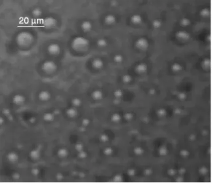
Sometimes in applied colloid science, the upper limit of size is extended to much larger values (e.g., several hundreds of micrometres). Examples are emulsions (Fig. 1.2.2) and foams.

Fig. 1.2.2 Emulsion of paraffin-oil in water (source: P. Ghosh, Colloid and Interface Science, PHI Learning, New Delhi, 2009; reproduced by permission).

Although the size of the particles is very small, a colloid dispersion is quite different from a solution. For example, a true solution passe through parchment or cellophane papers, but a colloid dispersion cannot; only the continuous medium of the dispersion seeps through. Some of the dispersions pass through an ordinary filter paper like a true solution. The particles of the dispersed phase can be viewed easily in an ultramicroscope or an electron microscope. They can be discerned by light scattering.

(4)

1.2.2 Various types of colloid dispersions with examples

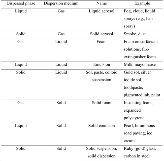
Some examples of colloid dispersions are given in Table 1.2.1. Table 1.2.1 Colloid dispersions

Dispersed phase Dispersion medium Name Example

Liquid Gas Liquid aerosol Fog, cloud, liquid

sprays (e.g., hair spray)

Solid Gas Solid aerosol Smoke, dust

Gas Liquid Foam Foam on surfactant

solutions, fire-extinguisher foam

Liquid Liquid Emulsion Milk, mayonnaise

Solid Liquid Sol, paste, colloid

suspension

Gold sol, silver iodide sol, toothpaste,

pigmented ink, paint

Gas Solid Solid foam Insulating foam,

expanded polystyrene

Liquid Solid Solid emulsion Pearl, bituminous

road paving, ice cream

Solid Solid Solid suspension,

solid dispersion

Ruby (gold) glass, carbon in steel

(5)

1.2.3 Classification of colloids

Freundlich (1926) classified the colloid systems into two categories: (i) lyophilic (or solvent-loving) colloids

(ii) lyophobic (or solvent-fearing) colloids

If water is the dispersion medium, the terms hydrophilic and hydrophobic colloids are used, respectively. Lyophilic colloid dispersions are formed quite easily by the spontaneous dispersion of the colloid particles in the medium. For example, the swelling of gelatin in water indicates the high affinity between the water and gelatin molecules. Classic examples of the lyophilic colloids are macromolecular proteins, micelles and liposomes. Lyophobic colloids do not pass into the dispersed state spontaneously. They are generally produced by mechanical or chemical action. An example of lyophobic colloid is latex paint.

Kruyt (1952) classified colloids as, (i) reversible colloids

(ii) irreversible colloids

For reversible colloids, the dispersed phase is spontaneously distributed in the surrounding medium by thermal energy. For example, a protein crystal dissolves in water spontaneously. Such spontaneous dispersion leads to an equilibrium size distribution corresponding to the minimum value of the thermodynamic potential. If the dispersed phase is thrown out of the colloid state, its redispersion is achieved easily. The irreversible colloid dispersions, on the other hand, are thermodynamically unstable. To illustrate, a gold crystal, if brought in contact with water, will not generate the sol spontaneously. The subdivision of the gold crystal into small particles can be performed only by supplying a considerable amount of energy. The total free energy of the goldwater interface is a positive quantity. The small entropic gain in the subdivision process is not sufficient to make the formation of sol spontaneous. This type of colloids has a natural tendency to be thrown out of the dispersion medium from the colloid state. Their stability in the colloid state is achieved with considerable difficulty.

(6)

1.2.4 Coagulation and flocculation

 The terms coagulation and flocculation are widely used in colloid chemistry to mean aggregation of the particles. The term coagulation to implies the formation of compact aggregates leading to the macroscopic separation of a coagulum, and the term flocculation is used implying the formation of a loose or open network which may or may not separate macroscopically.

 Various chemicals (e.g. polymers) are used to induce flocculation or coagulation. These are known as flocculants or coagulants.

 The intermolecular and surface forces play important roles in the stabilization and coagulation of colloids.

1.2.5 Critical coagulation concentration

 When the colloid particles are stabilized, the process is known as peptization. The reverse process, i.e., the destabilization of colloids is termed coagulation.

 Certain ions are necessary to cause peptization or coagulation.

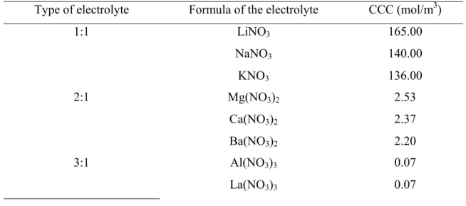
 The amount of electrolyte required to induce coagulation depends upon the valence of the counterion in the salt. This concentration of electrolyte is known as critical coagulation concentration (CCC) or flocculation value (see Table 1.2.2). Table 1.2.2 Critical coagulation concentrations of some salts for the negatively charged

AgI sol

Type of electrolyte Formula of the electrolyte CCC (mol/m3)

1:1 LiNO3 165.00 NaNO3 140.00 KNO3 136.00 2:1 Mg(NO3)2 2.53 Ca(NO3)2 2.37 Ba(NO3)2 2.20 3:1 Al(NO3)3 0.07 La(NO3)3 0.07

(7)

Ce(NO3)3 0.07

 The valence of the counterion is a very important parameter for the coagulation of a sol. The amount of divalent counterion required to coagulate the AgI colloid is much smaller than the amount of the monovalent counterion. The amount of trivalent counterion required is even less.

 The effect of valence of counterion on coagulation can be explained by the SchulzeHardy rule. It states that the critical coagulation concentration varies with the inverse sixth-power of the valence of the counterion. The specific nature of these ions is less important. Also, the effect of the valence of the coions (i.e., the ions of the electrolyte having the same charge as the colloid particles) is less significant on coagulation.

Example 1.2.1: The critical coagulation concentrations for NaCl, MgCl2 and AlCl3 for

negatively charged As2S3 colloids are 60 mol/m3, 0.7 mol/m3 and 0.09 mol/m3,

respectively. Verify whether these values are consistent with the SchulzeHardy rule or not.

Solution: Since the As2S3 colloid particles are negatively charged, the concentrations of

the cations are important. If we represent the concentrations of the monovalent, divalent and trivalent cations by c₁, c₂ and c₃, then from the given data on critical coagulation concentration, we have,

1: 2: 360 : 0.7 : 0.09 1: 0.012 : 0.0015

c c c

According to SchulzeHardy rule,

1: 2: 3 1: 1₆: 1₆ 1: 0.016 : 0.0014

2 3

 

c c c

(8)

1.2.6 Thermodynamic and kinetic stabilities of colloids

 Association colloids (e.g., surfactant micelles) and microemulsions are examples of thermodynamically stable colloidal systems.

 Many colloid systems are thermodynamically unstable. However, they are kinetically stable. The well-known examples are emulsions and foams. A system which shows resistance to coagulation is called kinetically stable colloid system.

 The term colloid stability generally implies kinetic stability.

1.2.7 Sedimentation in gravitational field

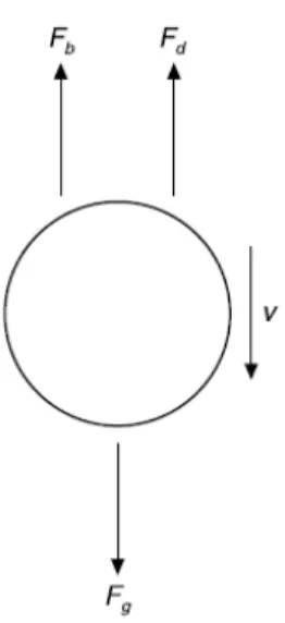
Let us consider the movement of an uncharged spherical particle through a liquid under the gravitational force (Fig. 1.2.3). For small colloid particles, the flow occurs at very low velocities relative to the sphere. This is known as creeping flow. Two other forces act on the particle: buoyant force and drag force, as shown in the following figure. The buoyant force acts parallel with the gravity force, but in the opposite direction.

Fig. 1.2.3 Forces acting on a colloid particle falling downwards by gravity.

The drag force appears whenever there is relative motion between a particle and the fluid. It opposes the motion and acts parallel with the direction of the movement, but in

(9)

Joint Initiative of IITs and IISc  Funded by MHRD 9/14 the opposite direction. Let us represent the gravity, buoyant and drag forces by F_g, F_b and F_d, respectively. Let the mass of the particle be m, and its velocity relative to the fluid be v. The resultant force on the particle is F_g F_bF_d. The acceleration of the particle is dv dt. Therefore, we can write the following force balance.

 _g  _b _d

dv

m F F F

dt (1.2.1)

The gravity force is,



g

F mg _(1.2.2)

By Archimedes’ principle, the buoyant force is the product of the mass of fluid displaced by the particle and the acceleration under gravity.

 b p mρg F ρ (1.2.3)

where ρ is the density of the liquid and ρ_p is the density of the particle. The drag force on the particle is given by Stokes’ law,

3



d

F πμvd (1.2.4)

where μ is the viscosity of the liquid and d is the diameter of the particle. Equation (1.2.4) is applicable when the particle Reynolds number



dvρ μ



is low (say, < 0.1). Two-thirds of the total drag on the particle is due to skin friction, and the rest is due to form-drag. From Eqs. (1.2.1)–(1.2.4) we get,

3       _ _   _ _    p p ρ ρ dv πμvd g dt ρ m (1.2.5)

When the particle settles under gravity, the drag always increases with velocity. The acceleration decreases with time and approaches zero. A small colloid particle quickly reaches a constant velocity after a very brief accelerating period. This is the maximum attainable velocity under the circumstances. It is known as the terminal velocity, v_t. The equation for v_t can be obtained by setting dv dt 0. Therefore, from Eq. (1.2.5) we get,

(10)

Joint Initiative of IITs and IISc  Funded by MHRD 10/14 3           p p t ρ ρ mg ρ v πμd (1.2.6)

Putting mπd g3 ρ_p 6 in Eq. (2.6), we get,





2 18   p t d g ρ ρ v μ (1.2.7)

This is the expression for terminal velocity based on Stokes’ law. It is evident that when



p

ρ ρ, the particle settles or sediments to the bottom (e.g., paint pigments settle to the bottom of a paint container). When ρ_p ρ, the converse is true and the particle rises, which is known as creaming (e.g., cream rises to the top of a bottle of milk). The derivation given in this section is based on the following assumptions.

(i) Settling is not affected by the presence of other particles in the fluid. This condition is known as free settling. When the interference of other particles is appreciable, the process is termed hindered settling.

(ii) The walls of the container do not exert an appreciable retarding effect.

(iii) The particle is large compared with the mean free path of the molecules of the fluid. Otherwise, the particles may slip between the molecules and thus attain a velocity that is different from that calculated.

If the particles are very small (~100 nm or less), Brownian movement becomes important. The effect of Browning movement can be reduced by applying centrifugal force. The concentrations of dispersions used in industrial applications are usually high so that there is significant interaction between the particles. As a result, hindered settling is observed. The sedimentation rate of a particle in a concentrated dispersion may be considerably less than its terminal falling velocity under free settling conditions.

1.2.8 Sedimentation in centrifugal field

It is easy to produce high acceleration in a centrifugal field so that the effects of gravity become negligible. The equation of motion for the particles in a centrifugal field

(11)

Joint Initiative of IITs and IISc  Funded by MHRD 11/14 is similar to the equation for gravitational field, except that the acceleration due to gravity needs to be replaced by the centrifugal acceleration rω2, where r is the radius of rotation and ω is angular velocity. Therefore, in this case the acceleration is a function of the position r. For a spherical particle obeying Stokes’ law the equation of motion is,





3 2 ₃ 6           p πd dr ρ ρ rω πμd dt (1.2.8)

As the particle moves outwards, the accelerating force increases. Therefore, it never acquires an equilibrium velocity in the fluid. Equation (1.2.8) can be simplified to give,





2 2 ₂ 18      _ _   p t d ρ ρ rω dr rω v dt μ g (1.2.9)

Thus, the instantaneous sedimentation velocity dr dt can be considered as the terminal velocity in the gravity field that is increased by a factor equal to the acceleration ratio,

2

rω g. Let us define a sedimentation coefficient

 

s as, 2

 dr dt

s

rω (1.2.10)

The sedimentation coefficient represents the sedimentation velocity per unit centrifugal acceleration. It can be determined by measuring the location of a particle along its settling path. Integrating Eq. (1.2.10), we get,







2 1



2 2 1 ln   r r s ω t t (1.2.11)

 Fine colloid particles sediment at a very slow rate under gravity. Swedish chemist Theodor Svedberg (Nobel Prize in Chemistry, 1926) developed a centrifuge which operates at a very high speed (e.g., 5000–10000 rad/s) generating an enormous centrifugal force. This force is much greater than the gravitational force. It is known as ultracentrifuge (Fig. 1.2.4).

 The dispersion is taken in a specially designed cell and vigorously whirled by special motors. The speed of rotation is so high that an acceleration as high as 106

(12)

Joint Initiative of IITs and IISc  Funded by MHRD 12/14 only hastens the sedimentation process, but it also separates the molecules on the basis of differences in mass, density or shape. The ultracentrifuge has proved to be very effective for macromolecular solutions, especially the proteins.

Fig. 1.2.4 Beckman L8-80M ultracentrifuge (photograph courtesy: Beckman Coulter India Pvt. Ltd.)

Example 1.2.2: A spherical particle suspended in water is placed in a centrifugal field. The diameter of the particle is 1107 m. What should be the rotational speed so that the particle moves from 6.5 cm to 7 cm in 60 s? Density of the particle is 7500 kg/m3. Solution: The sedimentation coefficient is given by,













 





2 7 2 9 3 1 10 7500 1000 3.6 10 18 _{18 1 10}            p d ρ ρ s μ s

The speed of rotation is,





1 2





1 2 2 1 9 ln ln 7 6.5 585.7 3.6 10 60     _ _ _ _         r r ω s t rad/s

(13)

Exercise

Exercise 1.2.1: Calculate the terminal velocity of a 10 m diameter carbon tetrachloride drop in water. Given: density of carbon tetrachloride = 1600 kg/m3, viscosity of water = 1 mPa s. What are the assumptions made in your calculation?

Exercise 1.2.2: A 1 m diameter quartz particle (density = 2650 kg/m3) suspended in water is placed in a centrifuge. The centrifuge rotates at a speed of 1000 rad/s. Calculate the sedimentation coefficient. What will be radial position of the particle with respect to its initial position after operating the centrifuge for 60 s?

Exercise 1.2.3: Answer the following questions.

i. Mention the forces which act on a colloid particle when it settles in liquid under gravity.

ii. What is terminal velocity?

iii. What is the difference between free settling and hindered settling? iv. What is creaming? When does it occur?

v. What is the advantage of centrifugal sedimentation over the gravitational sedimentation?

vi. Define sedimentation coefficient.

(14)

Colloidal Materials: Part I