How Volatile and Unpredictable are Aid Flows, and What are the Policy Implications?

(1)

Copyright ã UNU/WIDER 2001 * [email protected] and [email protected]

This is a revised version of the paper originally prepared for the UNU/WIDER development conference on Debt Relief, Helsinki, 17–18 August, 2001.

UNU/WIDER gratefully acknowledges the financial support from the governments of Denmark, Finland and Norway to the 2000-2001 Research Programme.

are Aid Flows, and What are the

Policy Implications?

Aleš Bulír and A. Javier Hamann*

December 2001

Abstract

This paper examines empirical evidence on the volatility and uncertainty of aid flows, and the main policy implications. Aid is found to be more volatile than fiscal revenues—particularly in highly aid-dependent countries—and mildly procyclical in relation to activity in the recipient country. These findings imply that the current pattern of aid disbursements is welfare-reducing. We also find that uncertainty about aid disbursements is large and that the information content of commitments made by donors is either very small or statistically insignificant. Policies to cope with these features of aid, as well as broader international efforts to reduce the volatility and procyclicality of aid, are briefly discussed.

Keywords: external aid, volatility, predictability, IMF-supported programs JEL classification: F35, O19

(2)

UNU World Institute for Development Economics Research (UNU/WIDER) was established by the United Nations University as its first research and training centre and started work in Helsinki, Finland in 1985. The purpose of the Institute is to undertake applied research and policy analysis on structural changes affecting the developing and transitional economies, to provide a forum for the advocacy of policies leading to robust, equitable and environmentally sustainable growth, and to promote capacity strengthening and training in the field of economic and social policy making. Its work is carried out by staff researchers and visiting scholars in Helsinki and through networks of collaborating scholars and institutions around the world.

UNU World Institute for Development Economics Research (UNU/WIDER) Katajanokanlaituri 6 B, 00160 Helsinki, Finland

Camera-ready typescript prepared by the authors and Adam Swallow at UNU/WIDER Printed at UNU/WIDER, Helsinki

The views expressed in this publication are those of the author(s). Publication does not imply endorsement by the Institute or the United Nations University, nor by the programme/project sponsors, of any of the views expressed.

ISSN 1609-5774

ISBN 92-9190-110-5 (printed publication) ISBN 92-9190-111-3 (internet publication)

Nowak, Matthew Odedokun, Tony Pellechio, T.N. Srinivasan and participants at the IMF Workshop on Macroeconomic Policies and Poverty Reduction held on April 12– 13, 2001, the WIDER conference on Debt Relief held on August 17–18, 2001, and the 57th Congress of the International Institute of Public Finance, held on August 27–30, 2001, for helpful suggestions. They also thank IMF desk officers for responding to their questionnaire. Siba Das, Patricia Gillett and Ivetta Hakobian provided excellent research assistance.

(3)

Prepared by Aleš Bulír and A. Javier Hamann1 October 2001

Abstract

This paper examines empirical evidence on the volatility and uncertainty of aid flows, and the main policy implications. Aid is found to be more volatile than fiscal revenues–

particularly in highly aid-dependent countries–and mildly procyclical in relation to activity in the recipient country. These findings imply that the current pattern of aid disbursements is welfare-reducing. We also find that uncertainty about aid disbursements is large and that the information content of commitments made by donors is either very small or statistically insignificant. Policies to cope with these features of aid, as well as broader international efforts to reduce the volatility and procyclicality of aid, are briefly discussed.

JEL Classification Numbers: F35, O19

Keywords: external aid, volatility, predictability, IMF-supported programs Author’s E-Mail Address: [email protected] and [email protected]

1_{The authors thank Craig Burnside, Domenico Fanizza, Dominique Guillaume, Henrik} Hansen, Tim Lane, Leslie Lipschitz, Russell Kincaid, Alex Mourmouras, Michael Nowak, Matthew Odedokun, Tony Pellechio, T.N. Srinivasan and participants at the IMF Workshop on Macroeconomic Policies and Poverty Reduction held on April 12-13, 2001, the WIDER conference on Debt Relief held on August 17-18, 2001, and the 57th Congress of the

International Institute of Public Finance, held on August 27-30, 2001, for helpful

suggestions. They also thank IMF desk officers for responding to their questionnaire. Siba Das, Patricia Gillett and Ivetta Hakobian provided excellent research assistance.

(4)

Contents Page

I. Introduction...3

II. Data Sources and Measurement Issues...5

A. The Data Set...5

B. The Composition of Aid...6

C. Common Denominator for Aid and Fiscal Revenue...9

D. The Time Series Properties of Aid and Revenue ...10

III. Measuring the Relative Variability of Aid and Revenue...10

IV. Predictability of Aid ...16

A. The Time Series Evidence ...16

B. How Good are Aid Projections in IMF-Supported Programs?...21

The Survey ...21

Results for project aid ...23

Results for program aid ...25

V. Conclusions and Policy Recommendations...28

Figures Figure 1. Frequency Distribution of the Cyclical Character of Aid ...15

Figure 2. Characteristics of Aid: Volatility, Cyclicality and Dependency ...17

Figure 3. Aid-dependent, Poor Countries and Countries with Volatile Aid also have Less Predictable Aid ...22

Figure 4. Frequency Distribution of Aid Disbursements...26

Figure 5. Prediction Errors of Aid in IMF Programs ...29

Tables Table 1. Relative Volatility of Aid and Revenue ...12

Table 2. Interdependence between Aid and Revenue Flows ...14

Table 3. Commitments are Poor Predictors of Actual Disbursements...20

Table 4. How Good are Short-term Aid Projections? ...24

Boxes Box 1. Components of Aid and their Economic Impact ...7

Box 2. Volatility and Composition of Aid: Malawi in the 1990s...8

Appendix Tables Table A1. Volatility of Aid and Revenue and the Aid-to-Revenue Ratio ...32

Table A2. Volatility of Aid and Revenue; Country Data...33

Table A3. Statistical Significance of Commitments in Forecasting Actual Disbursements....34

Table A4. List of Countries Used in the Survey...35

(5)

I. INTRODUCTION

This paper documents key cyclical properties of external aid flows from the point of view of the recipient country: their degrees of volatility and predictability, and the way in which they covary with domestic economic activity. Why the focus on the cyclical properties of aid? First, available estimates of the welfare cost of business fluctuations in developing countries suggest that they are significantly larger than those in industrial economies.2 Developing countries tend to be subject to more frequent and larger external shocks and are less able to cope with them due to pervasive liquidity constraints and the lack of effective countercyclical policy tools. A direct implication of this result is that advice to developing countries should pay more attention to reducing volatility. Second, these countries are also likely to be recipients of large volumes of aid disbursements of foreign aid, which have been found to be very volatile themselves (see below). This feature of aid can indirectly offset some of its direct beneficial effects by, for example, complicating the conduct of fiscal and monetary policy or exacerbating exchange rate variability (Edwards and van Wijnbergen, 1989). In particular, the negative welfare effects of volatile aid flows will be larger the higher the covariance between domestic output fluctuations and aid disbursements.3

In principle, the problem of aid volatility is analogous to that of volatility of commodity prices in countries that rely heavily on revenues from the exports of a single commodity. However, only a few, recent empirical studies have focused on the magnitude and consequences of aid volatility (and on best practices to deal with them) in contrast with the case of export price instability, where the main issues have been dealt with extensively in the economic literature.4_{Lensink and Morrisey (2000) find that the effect of aid on growth is} insignificant unless some measure of aid uncertainty is included in the regression, and that uncertainty about aid is detrimental to growth. Gemmell and McGillivray (1998) find that shortfalls in aid are most frequently followed by reductions in government spending, and sometimes by increases in taxes, or both. In other words, the typical aid-receiving country is

2_{Pallage and Robe (2001b) estimate that, on average, the welfare cost of output volatility in} Sub-Saharan Africa could be as much as 15-20 times higher that in the U.S.

3_{Assuming that government spending is financed only with tax revenues and foreign aid, it is} possible to show that the loss function of a risk-averse policymaker interested in minimizing deviations of public spending from planned levels is a positive function of the covariance between aid disbursements and actual revenues. We thank T.N. Srinivasan for this point. 4_{For example, Varangis and Larson (1996) provide a clear explanation of the problems} posed by commodity price uncertainty and clarify the differences among the main instruments to deal with price variability, unpredictability and expenditure smoothing. Similarly, Engel and Meller (1993) contain a set of case studies analyzing best policies to neutralize external shocks in developing countries (typically stabilization funds and the use of financial instruments).

(6)

unable to offset an unexpected non-disbursement of aid by borrowing, and has to resort to costly, and possibly inefficient, swift fiscal adjustment.5 Gemmell and McGillivray (1998) also find that aid is significantly more volatile than revenue and that, on average, aid tends to be procyclical (that is, countries tend to receive more aid in years when economic activity is on the rise; this, in turn, may imply a positive correlation between aid and fiscal revenues). These results are corroborated by Pallage and Robe (2001a) and suggest that the typical pattern of aid disbursement (highly volatile and procyclical) is likely to be welfare reducing.6 To the best of our knowledge, Collier (1999) is the only study that finds aid (in Sub-Saharan Africa) to be less volatile than tax revenues, and countercyclical.7

In this paper we re-examine these issues using a broader database than that used in the studies cited above (we use both publicly available time-series data as well as a cross-section of detailed data provided by IMF desk-officers of countries receiving aid). In line with the studies of Gemmell and McGillivray (1998) and Pallage and Robe (2001a), we find, first, that aid is substantially more volatile than either fiscal revenue or GDP and, further, that this relative volatility increases with the degree of aid dependency as measured by the aid-to-revenue ratio. We also find that aid tends to be mildly procyclical, and that countries that suffer from relatively high revenue volatility also exhibit higher volatility in aid receipts. These results suggest that aid tends to enhance budgetary and overall economic instability.

Second, time-series data show that commitments by donors exceed disbursements systematically and that aid cannot be predicted reliably on the basis of donors’ commitments alone. Cross-sectional data from IMF-supported programs reveal that commitment-based projections tend to overestimate project and, to a much higher degree, program aid. In addition, intra-year disbursements of program aid differ significantly from projections. Despite their poor track record as a predictor of disbursements, commitments continue to be used in budgetary exercises in aid recipient countries mainly as a result of pressures from donor countries and/or agencies.

Since the economic effects of aid are largely determined by the recipient country’s budgetary practices, we stress the need to account properly for aid volatility when designing

5_{Of course, incomplete adjustment to the shortfall in aid is likely to crowd out private} investment and/or create inflationary pressures (Hadjimichael et. al., 1995).

6_{We must stress here that the negative welfare effect referred-to above relates exclusively to} the cyclical movement of aid. Throughout this paper, we abstract from the issue of aid effectiveness, or even from the effect of aid volatility on growth. For a recent survey of those issues see, for example, Hansen and Tarp (2000, 2001).

7_{Collier (1999) is also the only study based on non detrended data. He takes his results to} imply that “a budget with a large component of aid would be more reliable than one with a low component of aid” (p. 542) and that all committed aid should be included in the budget.

(7)

adjustment programs in aid receiving countries—particularly when it comes to planning against the possibility of delays and/or shortfalls in aid disbursements vis-à-vis commitments. Finally, we discuss briefly measures that can be taken by both donors and aid-recipients— mainly in the areas of compliance with program objectives, program design, coordination among donors and improved disbursement procedures in donor countries—in order to reduce the volatility, procyclicality and unpredictability of aid and, thus, enhance its welfare effects.

The paper is organized as follows. Section II discusses briefly our data sources, as well as some problems posed by the need to select a common unit of measurement for several variables and the limitations of using aggregate data on aid. Section III looks at various measures of the relative instability of foreign aid and fiscal revenues. Section IV deals with the issue of predictability of aid flows and the information content of

commitments made by donors. This section also looks at the accuracy of predictions of aid made at various stages of a program supported by the donor community. Finally, Section V concludes with a discussion of the main policy implications of our findings.

II. DATA SOURCES AND MEASUREMENT ISSUES

Before turning to the assessment of the relative volatility and predictability of foreign aid, in this section we discuss the origin and scope of our data, as well as some problems associated with their measurement. These problems relate to the limitations of any empirical analysis based on aggregate aid estimates; problems linked to the selection of a common unit of measurement (denominator) for aid and domestic revenues; and the time-series properties of aid and revenue and the need to take them into account in order to measure volatility and predictability properly.

A. The Data Set

The data on aid used in this study were taken from the World Bank’s World

Development Indicators (WDI), which, in turn, are based on raw data compiled by the OECD and grouped under the heading of “Official Development Assistance” (ODA). The time series of commitments and actual disbursements of aid correspond to the line “Long-term funds by official and private donors, excluding IMF financing”. In principle, aid data are available for more than 100 countries, however, not all aid recipients represent relevant cases for the purposes of this study.

The pool of aid recipients changes over time. Within our sample period some former aid recipients became donors, others experienced a substantial change in their composition of aid, and several former communist countries joined the pool of aid recipients in the early 1990s. Thus, to compile a consistent database, we considered only cases that meet the following selection criteria: (i) at least eight annual observations available; (ii) presence of IMF-supported program(s) during the sample period; and (iii) population of at least 500,000.

(8)

The second criterion was intended to capture the mobilizing impact of IMF programs on aid flows and their composition.8 The third criterion was aimed at eliminating the small-country bias. These three criteria narrowed the potential sample to 72 countries for which aid data were available for the period 1975-1997 or some portion thereof.

Fiscal data used in the paper—total revenue in the local currency—were drawn from two sources. For the majority of countries (60), the series were obtained from the IMF’s International Financial Statistics (IFS). For the remaining 12 countries, mostly from sub-Saharan Africa and Asia, we used internal IMF data: in 10 cases we relied on the IMF’s African Department fiscal database, and in the other two the data were provided by IMF desk officers.9 Even with these additions, we were able to complete 1975-97 revenue series for only 47 countries; the available series are shorter for the other 25 countries (see Appendix Table A2).

B. The Composition of Aid

The OECD definition of ODA aggregates balance-of-payments support, capital projects, food aid, debt and emergency relief, peacemaking efforts, technical cooperation, concessional funding to multilateral development funds, and some other small categories of aid. More than 90 percent of the value of aid falls in the first two categories: some 50-60 percent is disbursed in the form of untied balance-of-payment support (the so-called program aid), while the remainder comes in the form of tied, project-related aid. These averages, however, may be affected by the presence of a few large recipients of program aid (say, Mexico in 1995 or Indonesia in 1998). Poor, aid-dependent countries generally have above-average proportions of project aid.

Given the high degree of heterogeneity among the components of aid, the use of an aggregate concept of aid is problematic, particularly when aid volatility is at the center of the discussion (Box 1 discusses the key macroeconomic differences between the two main categories of aid). For one thing, certain categories of aid are bound to be more volatile than others—for example, food aid is disbursed only during disaster periods—and, therefore, higher aggregate aid volatility may simply reflect shifts in the composition of total aid. In fact, aggregate volatility of aid may be high (low), even though the volatility of aid components may be low (high) when the covariance between the components is positive (negative) and relatively large (Box 2 illustrates this point in the case of Malawi).

8_{As explained below, most aid takes the form of project-related aid or untied, program aid.} The second category is practically non-existent in countries without IMF-supported

programs.

9_{The results obtained for these countries do not differ systematically from those obtained for} countries for which published data was available.

(9)

Box 1. Components of Aid and Their Economic Impact

Foreign aid is not a homogeneous variable, even though a popularly held view assumes that the fungibility of its various components makes it homogeneous. For example, aid earmarked for the construction of schools could free, ceteris paribus, financial resources for, say, military buildup. But what if aid is not fungible because the preferences of donors and aid recipients differ? The available evidence shows that the economic consequences of various forms of aid are not identical, see Lancaster (1999) for a review.

First, consider aid tied to specific investment projects. If donors' and

recipients' preferences are identical, the effect of project aid would be some increase in investment, imports, and budgetary spending on either tradables or nontradables— with the composition being decided by the preferences of domestic agents—as domestic fiscal resources earmarked for a project are replaced with aid. However, if aid is financing projects that the government would otherwise not have undertaken, the effect of aid would be simply the associated increase in investment and imports of tradables, with little or no impact on the domestic currency or absorption.

The second major category of aid is program aid. These funds could be considered totally fungible: additional program aid could finance higher spending, lower taxes, a reduction in debt, or a combination of all three, with the authorities deciding the composition. However, program aid finances typically additional spending on nontradable goods and, as such, that it has a strong impact on interest and exchange rates, often crowding out domestic absorption and hindering exports (Younger, 1992).

(10)

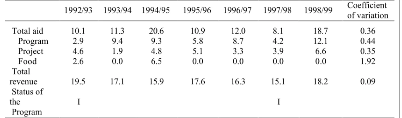
Box 2. Volatility and Composition of Aid: Malawi in the 1990s

Malawi is a good example of the complexity of aid flows. Aid, albeit significantly volatile, has been more stable on aggregate than two of its components (as suggested by the coefficients of variation shown below). Numerically, the lowest total aid receipts in any year have been 40 percent of maximum total aid receipts during that period and 62 percent of the average. However, the same ratios for program aid have been 35 percent and 56 percent and for project aid 29 percent and 44 percent, respectively. The ratios for total revenue have been much higher at 77 percent and 88 percent, respectively.

Table 1. Malawi: Various Types of Aid Flows, 1992/93-1998/99 (In percent of GDP) 1992/93 1993/94 1994/95 1995/96 1996/97 1997/98 1998/99 Coefficient _{of variation} Total aid 10.1 11.3 20.6 10.9 12.0 8.1 18.7 0.36 Program 2.9 9.4 9.3 5.8 8.7 4.2 12.1 0.44 Project 4.6 1.9 4.8 5.1 3.3 3.9 6.6 0.35 Food 2.6 0.0 6.5 0.0 0.0 0.0 0.0 1.92 Total revenue 19.5 17.1 15.9 17.6 16.3 15.1 18.2 0.09 Status of the Program I I

Sources: Malawian authorities; and Fund staff estimates and projections.

Note: ‘I’ indicate interruptions in the ESAF arrangement that affected disbursements during the whole fiscal year.

Aid is volatile also in the very short term. For example, during a period of less than two months in 1998/99, Malawi received about US$150 million of balance-of-payment support. This inflow of foreign exchange, which was more than twice as large as total disbursements during the previous 18 months, was equivalent to more than 150 percent of programmed reserve money or 11 percent of GDP. As a result, the Reserve Bank of Malawi had to undertake massive liquidity operations in order to prevent a triple-digits expansion of the monetary stock.

(11)

But there is an additional dimension to the aid heterogeneity problem: different forms of aid have different conditionality. For example, some aid is disbursed if an IMF-supported program is considered to be “on track”, others may have sector-specific conditionality and their disbursements depend on complex donor-recipient interactions. As a result, increased aid volatility may also reflect, to varying degrees, problems with project implementation, compliance with macroeconomic conditionality, or disruptions to the normal disbursement process originating in the donor country.

The literature offers little evidence on the empirical relevance of the points discussed above. On the one hand, insufficient data prevent comprehensive cross-country studies from differentiating among categories of aid. On the other hand, the few small-scale studies that have tried to decompose aid into various subcategories have either rejected parameter

constancy across regions (White, 1992 and Mosley et al., 1987 and 1992) or found the impact of aid to be insignificant in a cross-country set up (Mosley et al., 1992). Individual country studies are similarly inconclusive (see, for example, Pack and Pack, 1990 and 1993, for Indonesia and the Dominican Republic, respectively). In light of these results, we use the OECD composite definition of aid in Sections III and IV.A and investigate aid volatility and predictability separately for project and program aid in Section IV.B.

C. Common Denominator for Aid and Fiscal Revenue

Statistical measures of relative volatility are affected by the choice of a common denominator for aid and revenue. We use two alternative denominators for aid and revenue: percentages of GDP and current U.S. dollars in per-capita terms. From a domestic policy point of view, the percent-of-GDP denominator is more relevant as aid-receiving

governments generally do their financial programming either in domestic currency or in percentages of GDP rather than in U.S. dollars per capita. Moreover, the percent-of-GDP denominator captures better the impact of aid flows on exchange rate than the U.S. dollars per capita denominator. WDI data on GDP in local currency units, annual average market exchange rates, and population were used.

Why does the choice of a common denominator matter? Since our series for aid are denominated in U.S. dollars and those for revenues in domestic currency units, our

comparisons of volatility of aid and revenue are affected by another variable, namely the exchange rate.10 On the one hand, when expressing aid and revenue in U.S. dollars per capita, the volatility of domestic revenue becomes a composite measure of volatility of revenue in local currency terms and volatility of the exchange rate. On the other hand, when expressing the variables in percent of GDP, the volatility of aid becomes a composite measure of

10_{The impact of exchange rate volatility can be very large: on average, the volatility of the} exchange rate (measured by the coefficient of variation) in trended, raw data is almost forty times higher than that of aid.

(12)

volatility of aid in U.S. dollars, volatility of the exchange rate, and the impact of those variables on GDP.11 Thus, measures of relative volatility of aid tend to be lower when the series are expressed in U.S. dollars per capita, as compared to percentages of GDP. However, the implicit bias varies from country to country, as the volatility of the exchange rate between the domestic currency and the U.S. dollar tends to be larger in aid-receiving countries with floating exchange rates. As a result, due to the lack of a preferred scale variable for aid and revenue, we use both transformations, and keep in mind the biases that each of them are likely to introduce when interpreting our results.

D. The Time Series Properties of Aid and Revenue

Augmented Dickey-Fuller tests (not reported here but available upon request) indicate that the series for aid and revenue are generally nonstationary (or, in a few cases, stationary around a deterministic trend), and this finding is robust to the choice of the denominator. What are the implications of trends for measuring volatility? The standard statistics

(variance, the standard deviation, and the coefficient of variation) are designed for variables that revert to a constant mean and their application to trended data may result in serious biases. To avoid this problem, we detrended our aid and revenue series using the Hodrick-Prescott filter, and only then applied the usual measures of volatility.12

III. MEASURING THE RELATIVE VARIABILITY OF AID AND REVENUE

This section reviews our findings on the relative volatility of aid and domestic fiscal revenue. We calculate “trend-corrected” variances for aid and revenue, _θA_and

R

θ , respectively, and a measure of relative volatility defined as the ratio of the two,

R A _θ

θ /

=

Φ .

In the rest of this section we examine the properties of the measure of relative volatility, Φ. In particular, we: (i) calculate Φ for each country; (ii) look at the frequency distribution of individual country Φ’s and test the significance of averages and medians across countries;13_{(iii) test the relationship of}_Φ_{’s vis-à-vis other variables, such as the}

11_{Donors determine aid volumes either directly in U.S. dollars or in their own currencies,} which typically fluctuate much less vis-à-vis the U.S. dollar than currencies of aid-receiving countries, and, hence, the volatility of dollar-denominated aid is unaffected by the donors’ currencies exchange rate volatility.

12_{Following Pesaran and Pesaran (1997), we set the “smoothing” parameter}_λ_{at 7.}

13_{Since the distribution of}_Φ_{is not normal (it is bounded on the lower end), we checked the} statistical significance of sample averages using an F-test. The significance of sample

(13)

correlation coefficients between (detrended) aid and revenue (i.e., cyclicality of aid) and the ratio of (not detrended) aid to revenue (i.e., aid dependency); and (iv) in order to check the robustness of our results, we arrange countries into two sub-groups according to their degree of aid dependency, and compare the results for the full sample with those obtained for the smaller samples. Thus, we carry out our calculations not only for the full sample of 72 countries, but also for a sub-sample of countries with aid-to-revenue ratios of 10 percent or more (57 and 55 countries when measured in percent of GDP and U.S. dollars per capita, respectively) and also for a sub-sample of countries with aid-to-revenue ratios of 50 percent or more (33 and 29 countries when measured in percent of GDP and U.S. dollars per capita, respectively). The first cutoff point eliminates the more developed Latin American and Asian countries from the sample, while the second cutoff point defines a group of highly

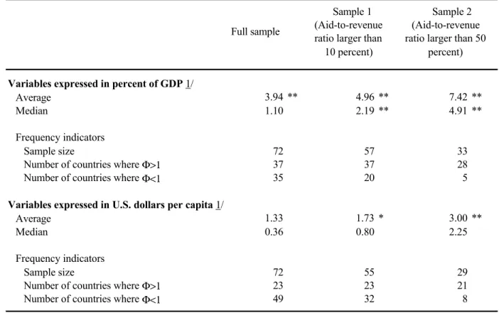
aid-dependent countries, mostly from Sub-Saharan Africa. The results are presented in Table 1. Our first finding is that aid is more volatile than revenue, particularly in countries with a high aid-to-revenue ratio. On the one hand, when variables are expressed in percent of GDP, aid is on average more volatile than revenue in all samples, and this result is

statistically significant (the F-test fails to reject the null hypothesis that the average Φ’s are larger than one at the 1 percent level of significance in every case).14 Furthermore, the relative volatility of aid grows with aid dependence: the average value of Φ increases from 3.94 to 7.42 as the sample is narrowed down to the most aid-dependent countries (the results for the median values of Φ follow a similar pattern). On the other hand, when the variables are expressed in U.S. dollars per capita, the average Φ is bigger than one in the full sample, but the difference from one is statistically insignificant. In the other two samples, aid is on average relatively more volatile than revenue and the results are statistically significant; again, the average value of Φ increases with aid dependency (from 11_/

3 to 3). The estimated

medians also grow as the sample is restricted to more aid-dependent countries, but they are not significantly different from one.15

We look also at the frequency of cases in which aid is more (or less) volatile than revenue and find stronger evidence in favor of a higher incidence of countries where aid is more volatile than revenue (Φ>1). When variables are expressed in percent of GDP, the share of countries with more volatile aid grows from about half in the full sample to about 2_/

3

in the middle sample, and well over 4_/

5 in the sample of the most aid-dependent countries. In

medians, which were used as another way to control for the non-normality of Φ, was

checked using a “runs test” (SPSS Inc., 1999, pp. 235-6).

14_{See Appendix Tables A1 and A2 for sample-specific and country-specific estimates of the} absolute volatility of aid and revenue.

15_{These results confirm that the choice of the scale variable matters. As predicted, when} variables are measured as a percentage of GDP, the estimated relative volatility of aid tends to be higher.

(14)

Table 1. Relative Volatility of Aid and Revenue (Φ)

Variables expressed in percent of GDP 1/

Average 3.94 ** 4.96 ** 7.42 **

Median 1.10 2.19 ** 4.91 **

Frequency indicators

Sample size 72 57 33

Number of countries where Φ>1 37 37 28

Number of countries where Φ<1 35 20 5

Variables expressed in U.S. dollars per capita 1/

Average 1.33 1.73 * 3.00 **

Median 0.36 0.80 2.25

Frequency indicators

Sample size 72 55 29

Number of countries where Φ>1 23 23 21

Number of countries where Φ<1 49 32 8

Source: Table A1 in Appendix [1].

1/ The null hypotheses that Φ > 1 is tested for averages with the F-test and for medians with the "runs test" ; '*' and '**' indicate statistical significance at the 5 and 1 percent level, respectively.

Full sample

Sample 1 (Aid-to-revenue ratio larger than

10 percent)

Sample 2 (Aid-to-revenue ratio larger than 50

(15)

the case of variables denominated in dollar-per-capita terms, there are more cases of aid being relatively less variable that revenues in the full and middle samples. In contrast, in the last sample, countries with higher relative aid volatility outnumber those with higher

volatility of revenue by a margin of 5 to 2.

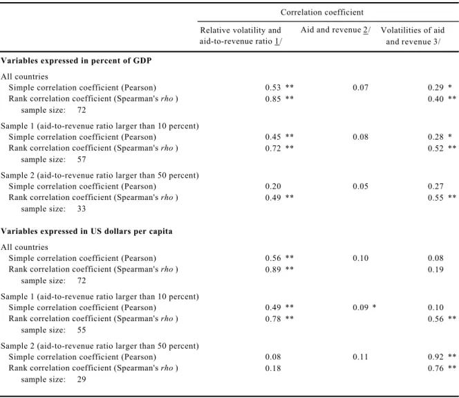
Second, we find that the relationship between the relative volatility of aid and aid dependency is robust.16_{The first column of Table 2 shows the correlation coefficients} between Φ and aid dependency in each of the three samples. The common denominator makes little difference in this case: the simple correlation coefficients between Φ and the aid-to-revenue ratio are of the order of 0.5-0.6 in the full sample, 0.5 in the middle sample, and a much lower 0.1-0.2 in the sample with aid-to-revenue ratios of 50 percent or more. The rank correlation coefficients (Spearman’s ρ) are about 0.7-0.9 in the full and middle samples and about 0.2-0.5 in the most aid dependent group. The positive correlation between the relative volatility of aid and aid dependency is statistically significant for all but the smallest sample. The lack of statistical significance in the smallest sample may reflect the fact that, by eliminating countries with a low aid-to-revenue ratio, we lower substantially the variance of the aid-to-revenue ratio series. In any case, we would stress that the average Φis about 20 times higher in the 10 most aid-dependent countries than in the 10 least aid-dependent countries.

Third, we find that, if anything, aid is modestly procyclical (second column of

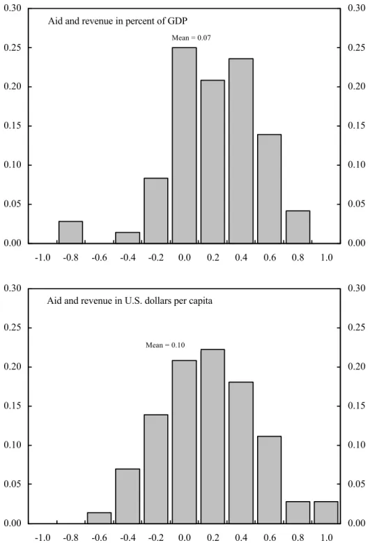
Table 2). The full-sample averages of individual correlation coefficients of detrended aid and revenue are positive, of similar size in all samples, but statistically insignificant in all but one case. However, a look at the distribution of correlation coefficients (Figure 1) reveals that they are concentrated to the right of zero and that only a small number of countries exhibit pronounced countercyclical pattern of aid. Furthermore, the share of countries with a

correlation coefficient smaller than –0.3 falls between 5 percent and 10 percent, whereas the share of countries with a correlation coefficient larger than 0.3 is 35-40 percent depending on whether the variables are expressed in percent of GDP or in U.S. dollars per capita. Thus, although the average results provide only weak support for the hypothesis that aid is procyclical, aid is found to be countercyclical only in a very small number of countries.

Finally, we find that shocks to domestic revenue are correlated with those to foreign aid (last column of Table 2). The correlation coefficients between the variances of aid (_θA₎

and revenue (_θR_{) are stable at about}_a_{for the variables in percent of GDP and grow from}

16_{A closer look at the data (Appendix Table A1) reveals that this result is not driven by} lower absolute revenue volatility in aid-dependent countries. For example, narrowing the full sample to countries with aid-to-revenue ratios of more than 50 percent leads to increases in average absolute aid volatility of 90 percent and 80 percent when variables are expressed in percent of GDP and in dollar-per-capita terms, respectively. By comparison, revenue volatility increases by 80 percent and declines by 97 percent, respectively.

(16)

Table 2. Interdependence Between Aid and Revenue Flows

(Aid and revenue are measured as differences from its Hodrick-Prescott filter) Correlation coefficient

Relative volatility and Aid and revenue 2/ Volatilities of aid aid-to-revenue ratio 1/ and revenue 3/ Variables expressed in percent of GDP

All countries

Simple correlation coefficient (Pearson) 0.53 ** 0.07 0.29 * Rank correlation coefficient (Spearman's rho) 0.85 ** 0.40 **

sample size: 72

Sample 1 (aid-to-revenue ratio larger than 10 percent)

Simple correlation coefficient (Pearson) 0.45 ** 0.08 0.28 * Rank correlation coefficient (Spearman's rho) 0.72 ** 0.52 **

sample size: 57

Simple correlation coefficient (Pearson) 0.20 0.05 0.27 Rank correlation coefficient (Spearman's rho) 0.49 ** 0.55 **

sample size: 33

Variables expressed in US dollars per capita All countries

Simple correlation coefficient (Pearson) 0.56 ** 0.10 0.08 Rank correlation coefficient (Spearman's rho) 0.89 ** 0.19

sample size: 72

Simple correlation coefficient (Pearson) 0.49 ** 0.09 * 0.10 Rank correlation coefficient (Spearman's rho) 0.78 ** 0.56 **

sample size: 55

Simple correlation coefficient (Pearson) 0.08 0.11 0.92 ** Rank correlation coefficient (Spearman's rho) 0.18 0.76 **

sample size: 29

Source: IFS, World Development Indicators, AFR fiscal database; and Fund staff calculations. Note: '*' and '**' indicate statistical significance at the 95 percent and 99 percent level, respectively. 1/ Correlation coefficient between each country's Φ and its aid-to-revenue ratio.

2/ Average of individual countries' correlation coefficients between detrended aid and revenue. 3/ Correlation coefficient of each country's aid and revenue variances (θ).

(17)

Figure 1. Frequency Distribution of the Cyclical Character of Aid 1/

(Relative frequency)

Source: Table A2.

1/ Measured by the correlation coefficient of aid and domestic fiscal revenue. Aid and revenue in percent of GDP

0.00 0.05 0.10 0.15 0.20 0.25 0.30 -1.0 -0.8 -0.6 -0.4 -0.2 0.0 0.2 0.4 0.6 0.8 1.0 0.00 0.05 0.10 0.15 0.20 0.25 0.30 Mean = 0.07

Aid and revenue in U.S. dollars per capita

0.00 0.05 0.10 0.15 0.20 0.25 0.30 -1.0 -0.8 -0.6 -0.4 -0.2 0.0 0.2 0.4 0.6 0.8 1.0 0.00 0.05 0.10 0.15 0.20 0.25 0.30 Mean = 0.10

(18)

0.2 to 0.9 when the variables are denominated in dollars per capita. While the sign of the correlation coefficient might have been expected, the size of the correlation coefficients and their stability across different samples are surprising. These results further undermine the notion that aid tends to smooth out shocks to revenue.

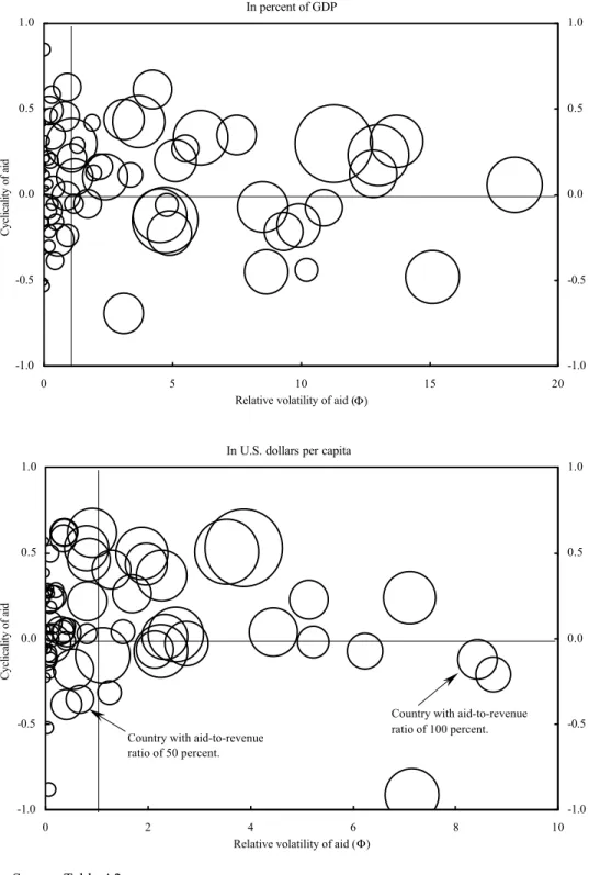
We summarize our main results graphically in Figure 2, where the top panel corresponds to variables expressed in percent of GDP and the bottom panel to variables denominated in dollars per capita. Each panel captures three dimensions: on the horizontal axis we plot the relative volatility of aid, Φ; on the vertical axis the correlation coefficient of aid and revenue (cyclicality of aid); and each observation is represented by a bubble whose size indicates the country’s aid-to-revenue ratio. First, we observe that aid is more volatile than revenue in countries with high aid dependency, as most of the “larger” bubbles are to the right of the vertical line Φ=1. Second, aid appears to be procyclical, as the majority of bubbles are above the horizontal line corresponding to a zero correlation between aid and revenue. Moreover, in only a few aid-dependent countries, that is, those with “larger” bubbles, aid is countercyclical. This pattern of cyclicality is more pronounced in the bottom panel, where aid and revenue are measured in dollar-per-capita terms.

IV. PREDICTABILITY OF AID

In this section we establish some stylized facts regarding the predictability of aid both, in general, and in the context of IMF-supported programs. To this end, we carry out two separate exercises. The first one is based on time-series data on aid disbursements and commitments in current U.S. dollars, and seeks to assess the information content of

commitments in the context of a simple auto-regressive model for aid disbursements. Available time series were typically longer in this case, as there was no need to compute them as a percentage of GDP, or constrain them to be of equal length as revenue series. The second exercise is based on responses to a questionnaire by IMF country desk economists. The results of this questionnaire allow us to test whether there are systematic differences between commitments made by donors, projections prepared in the context of IMF-supported programs, and actual disbursements.

A. The Time Series Evidence

Before turning to the estimation of the marginal contribution of commitments, C, to the prediction of disbursements, D, we would like to provide some basic information on these two variables for our sample of 72 countries. A simple look at individual-country plots of their C and D series (available upon request) reveals two salient features: (i) several episodes of spikes in commitments that, generally, were not followed by increased disbursements; and (ii) a systematic tendency for commitments to exceed disbursements.

The first point reflects a propensity for donors to react, in terms of large increases in commitments but not necessarily in disbursements, to positive changes in recipient countries, such as in the Central African Republic following the end of Bokassa’s regime in the early

(19)

Figure 2. Characteristics of Aid: Volatility, Cyclicality, and Dependency

(The size of the bubble indicates the aid-to-revenue ratio)

Source: Table A2.

In percent of GDP -1.0 -0.5 0.0 0.5 1.0 0 5 10 15 20

Relative volatility of aid (Φ)

Cyclicality of aid -1.0 -0.5 0.0 0.5 1.0

In U.S. dollars per capita

-1.0 -0.5 0.0 0.5 1.0 0 2 4 6 8 10

Relative volatility of aid (Φ)

Cyclicality of aid -1.0 -0.5 0.0 0.5 1.0

Country with aid-to-revenue ratio of 50 percent.

Country with aid-to-revenue ratio of 100 percent.

(20)

1990s or the end of the civil war in Mozambique in the mid-1990s. The exception to the second point are mainly (but not exclusively) a relatively small number of instances within our sample in which a country has received some form of financial help following an unforeseen balance of payments crisis. These cases, however, are concentrated among countries with relatively higher levels of income per capita and capital mobility, and low aid dependency. For the other countries in our sample, the C-to-D ratio was larger than one (i.e., commitments exceed disbursements), with the implicit average overprediction of

disbursements reaching up to 20 percent.17

While the simple calculations discussed above reveal that commitments tend to overestimate disbursements by a relatively wide margin, they do not say much about the information value of a commitment figure for predicting aid for the budget. In order to assess the marginal value of aid commitments in predicting aid disbursements, we estimated the following equation for the same sample of countries as in the previous section:

, 1 0 t i t t K i i t

D

C

T

D

=

β

+

β

₋

+

γ

+

δ

+

ε

=

∑

(1)

where T is a time trend and K represents the lag length. The ability of commitments to help predict the future course of disbursements is tested through the statistical significance of γ in this very simple forecasting equation for disbursements.18 We would expect that γ should be not only statistically significant but also positive and close to one if commitments contained high marginal information value. Of course, there are no simple a priori interpretations for the possible failure of γ to be significantly different from zero. Potential reasons for the failure of commitments to materialize include, inter alia, non-compliance by the receiving country with conditions attached to committed aid, delays associated with administrative problems in donor countries, or simply changes in underlying economic and/or political developments. Whatever the case, though, we think that it is important to document the predictive power of a variable that is widely used in fiscal programming exercises mainly in response to pressure from donors.

17_{Of the 71 countries in the sample (Cambodia had to be excluded from this exercise due to} the small number of observations available), only 18 received on average more aid than was committed. Of these, half have very low aid-to-revenue ratios and are among the best known cases of balance of payments crisis-related financial assistance (Argentina, Brazil, Ecuador, Mexico, Indonesia, Philippines, Thailand, Turkey, and Venezuela).

18_{We want to emphasize here that the purpose of this exercise is not to develop an elaborate} forecasting model for disbursements but, instead, to test the significance of commitments in the context of a parsimonious model. The equation was estimated using aid data on current U.S. dollars.

(21)

Given the nonstationarity of Ct and Dt, the parameter γ was estimated by running

equation (1) in first differences. The estimation process was carried out in two steps. In a first step, two alternative values of K were selected from a version of equation (1) that did not include Ct: those that minimized the Akaike Information Criterion (AIC) and the

Schwartz-Bayes Information Criterion (SBIC). The value of γ was then estimated by adding Ct as a

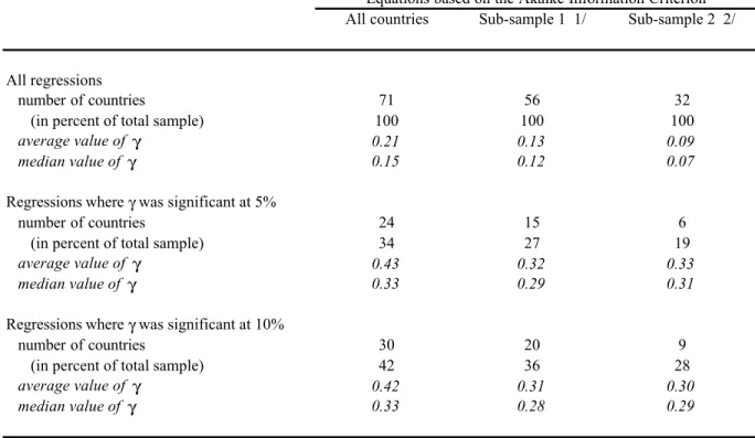
regressor in the resulting equations.19_{The results obtained using the AIC are summarized in} Table 3; there are no substantial differences between the results obtained under the AIC and those obtained under the SBIC.

In general, the estimated γ’s are not statistically significant, especially in countries with higher aid-dependency ratios. When all countries are considered, γ is significant at the 5 percent level in about a of the regressions.20 In these cases, the average value of γ is about

0.4; however, the median value is smaller (about a), reflecting the fact that the estimated value of γ was quite large for only a few countries: γ was higher than 0.7 in 5 higher-income countries with very low aid-to-revenue ratios (Argentina, Mexico, Panama, Turkey, and Venezuela).21 The estimated values of γ decreased (and the difference between their average and median values narrowed significantly) when the sample of countries was reduced to cases in which aid represents at least 10 percent of revenues. The estimated value of γ did not change further when the sample was reduced to countries where aid represents at least 50 percent of revenues, but the share of regressions with γ’s significant at the 5 percent level fell from about a in the full sample to about 1_/₅_{. When the level of statistical significance is}

lowered to 10 percent, none of the conclusions described above changes significantly. Two main conclusions can be drawn from Table 3. First, the marginal predictive power of commitments made by donors is statistically significant only in a relatively small fraction of the countries in our sample, and this fraction falls as the sample is reduced to countries where aid is relatively important. Second, even among countries where

commitments contain statistically significant information about future disbursements, the results suggest that commitments should not be taken at face value, but instead should be discounted heavily.

Finally, in line with the results of section III, we explored the relationship between predictability of aid, as measured by γ, and a few other variables. The top two panels of Figure 2 plot the estimated values of γ against the aid-to-revenue ratio and GDP per capita, respectively (the panels show also a fitted regression line and the estimated regression

19_{As a general rule, the initial number of lags was determined as one third of the available} number of observations.

20_{In one case, Thailand,}_γ_{is negative and statistically significant.}

(22)

All countries Sub-sample 1 1/ Sub-sample 2 2/ All regressions

number of countries 71 56 32

(in percent of total sample) 100 100 100

average value of γ 0.21 0.13 0.09

median value of γ 0.15 0.12 0.07

Regressions where γ was significant at 5%

median value of γ 0.33 0.29 0.31

Regressions where γ was significant at 10%

median value of γ 0.33 0.28 0.29

1/ Countries where aid represents more than 10 percent of government revenues. 2/ Countries where aid represents more than 50 percent of government revenues.

(Estimated values of γ in italics)

Table 3. Commitments are Poor Predictors of Actual Disbursements

(23)

coefficient). The relationship is negative in the first case, positive in the second case, and the estimated regression coefficients are statistically significant at the 1 percent level. These results show quite clearly that the predictive power of donors’ commitments tends to be lower in poorer and in more aid-dependent countries. The bottom two panels of Figure 3 plot the estimated γ’s against the two measures of relative aid volatility (Φ). In both cases, the relationship is negative, albeit not statistically significant, indicating only a weak correlation between volatility and unpredictability.

B. How Good are Aid Projections in IMF-Supported Programs? The Survey

The results in this section are based on responses by 37 IMF desk economists to a questionnaire sent in late 1999 (see Appendix Table A4 for a list of the countries). The questionnaire requested information on project and program aid for the most recent program period. The majority of the 37 countries in the sample drew financial support from the IMF under the Enhanced Structural Adjustment Facility (ESAF) and a few under General

Resource Account facilities. It must be stressed that, although the definition of aid employed in this questionnaire was intended to be as close as possible to that used by the OECD, in many cases the IMF estimates of aid inflows are somewhat smaller. This discrepancy mostly reflects the asymmetric nature of information on aid between donors and recipients: data on such components as technical assistance, peacemaking efforts, and other smaller categories of aid are often not reported to the recipient country and, hence, are not recorded in the countries’ fiscal and balance of payments accounts (on which the responses to our questionnaires are based).

We received data on project aid at four different junctures related to the life of a program, and recorded them under the following labels: (1) “Original projections”, prepared by the IMF staff about a year ahead of the start of the program. These projections are based on information on past disbursements as well as preliminary and heavily discounted donor commitments.22 (2)“Budget projections,” that is, the authorities’ projection at the time of the budget presentation, which usually takes updated commitments by donors at face value. (3) “IMF-program projection,” that is, the IMF staff estimate embedded in the financial program. Staff of the IMF generally incorporates some 90-95 percent of updated project aid

commitments into their fiscal projections. (4) “Disbursements”, as recorded by the authorities.

Regarding program aid, we received data at the same junctures as in the case of project aid, except for the budget estimates, which are generally identical to IMF projections.

22_{This figure can be thought of as corresponding to the first year of the medium-term} projections generated in an existing program or, in the case of countries that did not have an ongoing program, a set of estimates used at the start of a negotiation process that would lead to the adoption of a program over the next year.

(24)

Figure 3. Aid-Dependent, Poor Countries And Countries With Volatile Aid Have Also Less Predictable Aid

Source: Authors' own estimates.

Notes: The slope of the regression line is denoted by β. '*' and '**' indicate statistical significance at the 5 and 1 percent level, respectively.

Predictability of aid and aid dependency -1.0 -0.5 0.0 0.5 1.0 1.5 2.0 0 100 200 300 400

Aid-to-revenue ratio in percent

Estimated γ 's -1.0 -0.5 0.0 0.5 1.0 1.5 2.0

Predictability of aid and GDP per capita

-1.0 -0.5 0.0 0.5 1.0 1.5 2.0 0 2,000 4,000 6,000 8,000 GDP per capita Estimated γ 's -1.0 -0.5 0.0 0.5 1.0 1.5 2.0

Predictability and volatility of aid (I)

-1.0 -0.5 0.0 0.5 1.0 1.5 2.0 0 5 10 15 20 Average Φ in percent of GDP Estimated γ 's -1.0 -0.5 0.0 0.5 1.0 1.5

2.0 Predictability and volatility of aid (II)

-1.0 -0.5 0.0 0.5 1.0 1.5 2.0 0 2 4 6 8 10

Average Φ in dollar-per-capita terms

Estimated γ 's -1.0 -0.5 0.0 0.5 1.0 1.5 2.0 β = -0.14** β = 0.11** β = -0.01 β = -0.02

(25)

Specifically, we have data for: (1) “Original projections” (one-year-ahead projections

prepared by IMF staff, conditional on past disbursements and heavily discounted preliminary donor commitments); (2) “IMF-program projections” (non-discounted, updated commitments provided by donors);23_{and (3) “Disbursements”. Unlike in the case of project aid, for}

program aid we were able to obtain also a quarterly breakdown of each of the three annual projections.

Not all low-income countries with IMF-supported programs receive both project and program aid, and in some cases the distinction between the two is not made.24_{Also, a few} country desks did not report data that correspond to the definitions of “Original projections” or “Budget projections” described above. As a result, we do not have a balanced data set. For project aid we obtained: 27 observations for Original projections, 32 for IMF-program projections, 24 for Budget projections and 32 for Disbursements. For program aid, we obtained: 23 observations for Original projections, 28 for IMF-program projections and 28 for Disbursements. In order to have a common denominator, all data were expressed in percentages of the IMF-program projections.

Results for project aid

The average Disbursements of project aid fall short of all types of projections (Table 4).25 The ranking of errors in projections vis-à-vis Disbursements is unambiguous: Budget projections are the worst with an average error of 15 percent; IMF-program projections are the most accurate, with an average error of 5 percent; while Original projections come, quite surprisingly, in the middle with an average error of almost

8 percent.26_{Interruptions in IMF programs appear to have no statistically significant impact}

23_{Unlike project aid, program aid commitments (and disbursement dates) are updated} constantly; thus, in this case, the figure for “IMF-Program Projection” refers to the number used in the IMF Board meeting documents.

24_{There are reasons to believe that project aid data are of lower quality than those for}

program aid. Project aid disbursements generally take the form of paying invoices from third parties such as construction companies, importers, consultants, and so on. Reporting of these payments to aid receiving countries is often delayed and occasionally incomplete; some countries even lack their own independent systems for project aid monitoring. In contrast, program aid disbursements are recorded as a cash transfer in recipient countries’ central banks and, as such, can be easily monitored.

25_{While the original projections are fairly close to program projections (higher by only about} 22 percent), budget estimates were almost 10 percent higher than program projections, and IMF projections 5 percent higher.

26_{For project aid, one percentage point of prediction error amounts to about 0.1 percent of} GDP (the average IMF-program projection was 5.2 percent of GDP and the average “Disbursement” was 4.8 percent of GDP).

(26)

(In percent of IMF program projections, sample averages) Original projections (one-year-ahead IMF projections) Budget projections (authorities' commitment-based projections) Disbursements (as provided by the authorities) Project aid 1/ All countries 102.6 109.5 94.9 Of which:

Without program interruptions 105.2 109.1 94.9

With program interruptions 2/ 88.0 111.6 94.8

Program aid (annual data) 3/

All countries 100.9 . . . 68.5

Of which:

Without program interruptions 106.2 . . . 73.8

With program interruptions 2/ 65.5 . . . 33.8

Of which: 4,5/

Grants

Of which:

With program interruptions 6/ . . . .

Loans

Of which:

With program interruptions 65.5 . . . 4.9

Program aid (quarterly data) 7/

All countries . . . 49.3

Of which:

Without program interruptions . . . 46.2

With program interruptions 2/ . . . 82.5

1/ Data for 27 countries for original projections, 24 countries for budget projections, and 31 countries for actual outturns.

2/ Data for 4 countries. In one country, no program aid was committed and none was disbursed. 3/ Data for 23 countries for original projections and 26 countries for actual outturns.

4/ Because some country data do no have breakdown for grant and loans, the sum of grants and loans does not equal to the total program aid.

5/ Grant and loan data are available for 19 and 24 countries, respectively. 6/ Averages are not reported, because only one observation was available. 7/ Average deviation from the quarterly IMF-program projection.

(27)

on project-aid Disbursements. The fact that Budget projections fare the worst even though they are prepared relatively late in the process—and, presumably, with updated

commitments—reflects the pressure exerted by donors for aid recipient countries not to discount their commitments.

A closer look at the distribution of Disbursements as percentages of IMF-program projections (Figure 4, top panel) reveals that, while all projections overestimated

Disbursements on average, there were plenty of cases in which Disbursements were actually underestimated. Out of the 32 countries for which we had data on IMF-program projections and Disbursements, 18 countries had their project aid Disbursements fall short of IMF-program projections by about 20 percent of IMF-program projections, while 14 countries had project aid Disbursements that exceeded IMF-program projections by roughly the same magnitude.

Results for program aid

Program aid shortfalls vis-à-vis IMF projections are more marked: both Original and IMF-program projections overestimated Disbursements on average by more than 30 percent (despite some variations in individual cases, original and program projections are practically identical on average).27 The explanation for the much larger prediction errors in program aid projections as compared to project aid lies in the different nature of conditionality associated with the two types of aid. Unlike project aid, which flows gradually according to

multiple-year disbursement schedules and entails direct monitoring by donors of some large projects, program aid is generally disbursed only if the IMF-supported macroeconomic program is on-track (it is held back if the program is off-track). For this reason, in the case of program aid, it may be useful to look separately at programs with and without interruptions due to breaches in conditionality.

The difference in type of conditionality, however, does not account fully for the much more pronounced over-projections in the case of program aid. While countries with program interruptions (Central African Republic, Republic of Congo, Zambia, and Papua New

Guinea) received, on average, only about one-third of program aid commitments, successful, uninterrupted programs received still only three-quarters of program aid commitments.28 So, what explains the substantial shortfall vis-à-vis program projections in programs that

remained officially “on track”? There are three possible explanations: (i) program-aid

shortfalls originated in donor countries and are not related to recipient countries’ compliance

27_{For program aid, one percentage point of prediction error amounts to about 0.05 percent of} GDP (the average IMF-program projection was 4.7 percent of GDP and the average

“Disbursement” was 3.2 percent of GDP).

28_{Interestingly, in the group of interrupted programs original projections were some} 35 percent smaller than IMF-program projections, perhaps reflecting original skepticism about the prospects of the country securing and adhering to a program.

(28)

Figure 4. Frequency Distribution of Aid Disbursements 1/ (In percent of program projections)

Source: IMF questionnaire; authors' calculations.

1/ The samples contain 33, 28, and 23 countries, respectively. Excluding countries with no disbursements and countries with program interruptions.

2/ Average deviation from the quarterly projection. Project Aid Average 0.00 0.05 0.10 0.15 0.20 0.25 0.30 0 10 20 30 40 50 60 70 80 90 100 110 120 130 140 150 160 170 180 190 200 Relative frequency 0.00 0.05 0.10 0.15 0.20 0.25 0.30

Program Aid (Annual Data)

Average 0.00 0.05 0.10 0.15 0.20 0.25 0.30 0 10 20 30 40 50 60 70 80 90 100 110 120 130 140 150 160 170 180 190 200 Relative frequency 0.00 0.05 0.10 0.15 0.20 0.25 0.30

Program Aid (Quarterly Data) 2/

0.00 0.05 0.10 0.15 0.20 0.25 0.30 0 10 20 30 40 50 60 70 80 90 100 Relative frequency 0.00 0.05 0.10 0.15 0.20 0.25 0.30 Average Projections = disbursements Projections = disbursements Projections = disbursements

(29)

with donor conditionality; (ii) aid recipient countries breached donor conditionality, but not that associated with the IMF-supported program; or (iii) the overestimation reflects strategic behavior by the IMF, given its unique role as arbiter of external assistance. Unfortunately, we do not have information to assess the relative importance of these hypotheses.

The average result of excessively optimistic projections at all junctures is more representative in the case of program aid than for project aid (Figure 4, middle panel). Out of the 28 countries for which we received data on IMF-program projections and outcomes, 24 countries saw their Disbursements fall short of IMF-program projections (by an average of 42 percent of IMF-projected program aid), while only 4 countries recorded program aid Disbursements in excess of IMF-program projections (by an average of 14 percent). The overestimation of Disbursements exceeded 20 percent in only two countries.

Yet another way of dissecting our results is to compare prediction errors for program loans and program grants separately. Aside from differentiating aid that is debt neutral (grants) from aid that contributes to debt creation (loans),29 this analysis allows us to compare prediction errors vis-à-vis bilateral and multilateral donors. The differentiation in our data is not perfect, however. On the one hand, only bilateral donors disburse grants. On the other hand, loans are disbursed both by bilateral and multilateral donors. Still, the results show that bilateral aid in the form of program grants—which comprise about one-third of total program aid—has a much smaller prediction error than program loans, both bilateral and multilateral (bottom part of Table 4). While grant disbursements are lower that program projections by almost 13 percent, the corresponding estimate for loan disbursements is almost 40 percent. Also the shortfall vis-à-vis the original projection is much smaller for grants than for loans. We should mention, however, that the sample size is much smaller than in previous cases (19 and 24 countries for grants and loans, respectively), primarily because the breakdown of program aid is not available for some countries.

Program aid not only falls significantly short of the programmed level, but its

quarterly distribution also differs substantially from the programmed path (Figure 4, bottom panel). On average, actual quarterly outturns deviate by about 50 percent from the quarterly path estimated at the beginning of the program period. In other words, if, according to the program, a country expects to receive 10 million dollars in a given quarter, it gets, on average, either 5 million or 15 million. Out of 23 countries for which quarterly data are available, only 2 countries received program aid with prediction errors lower than 20 percent

29_{From a net-present-value perspective, aid in the forms of loans and grants may differ} relatively little. Even though loans will have to be repaid eventually, concessional lending is quite generous: interest rates are very low and the loan contracts usually offer extended grace periods.

(30)

(using the previous numerical example, only 2 countries could expect to get either 8 or 12 millions of U.S. dollars per quarter).30

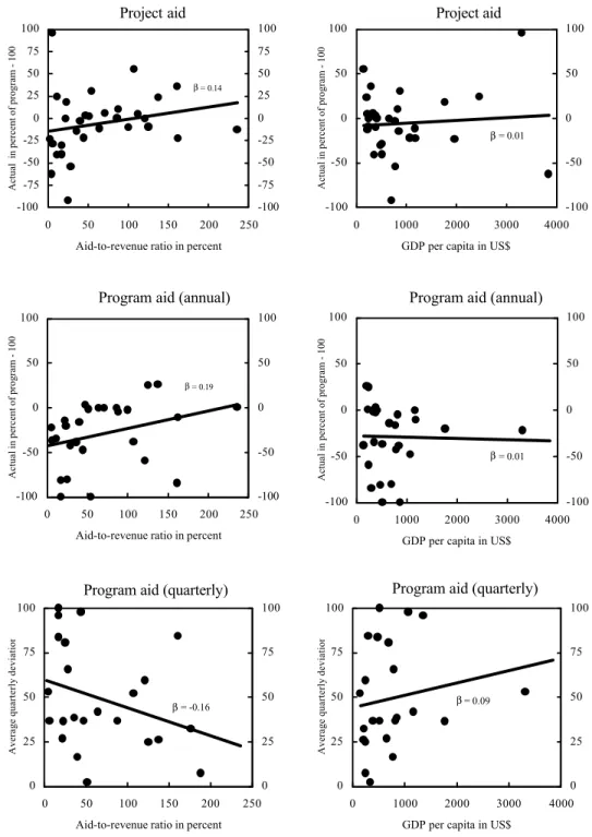
Unlike the case of donors’ commitments in the context of our “naive” prediction model (Section IV.A), the IMF-program projections of aid do not exhibit any systematic relationship vis-à-vis either aid dependency or the level of development. Figure 5 plots differences between IMF-program projections and Disbursements (expressed in percent of the former), against those two variables, separately for project aid and program aid, the latter in annual and quarterly frequencies. Although project and annual program aid prediction errors seem to be smaller in countries with lower aid-to-revenue ratios, the correlation is not statistically significant (top two left panels). Second, project and annual program aid

prediction errors appear to be completely unrelated to the level of development—the slopes of the fitted lines on the right, top two panels are flat and their values are statistically insignificant. Finally, the quarterly prediction errors (bottom panels) appear to be declining with the aid-to-revenue ratio, and increasing with the level of development, but, again, these results are not statistically significant.

The results from our questionnaire suggest that official projections of aid (including those of the IMF) are subject to large errors and that, particularly in the case of program aid, they seem to exhibit a substantial upward bias. It is somewhat ironic that even with the heavy discount of preliminary donors’ commitments embedded in the IMF staff’s Original

projections, for which the IMF staff is often criticized, those projections tend to overestimate Disbursements significantly. Original and IMF-program projections have, on average, practically identical forecast errors and, hence, it appears that the additional information that should in principle be provided by updated commitments at the beginning of the program period, adds in fact very little to the Original projections. The intra-year volatility of program aid was found to be remarkably high.

V. CONCLUSIONS AND POLICY RECOMMENDATIONS

In this paper we assess empirically various aspects of the cyclical behavior of aid flows. Although the welfare implications of highly volatile and unpredictable aid flows can be substantial—especially in countries that receive large volumes of aid—the issue has not received enough attention in the literature. Our findings suggest that the typical pattern of disbursement of aid tends to enhance budgetary and, possibly, overall economic instability, and reduce welfare. Before summarizing these findings, however, we would like to stress our hope that this paper will stimulate further research, particularly in assessing the robustness of our results to changes in detrending methods, the specific definition of aid flows or even the

30_{This calculation was made excluding the countries with program interruptions. The} average deviation in countries with program interruptions was more than 80 percent.

(31)

Figure 5. Prediction Errors of Aid in IMF Programs

(In percent of program projections)

Source: Authors' calculations.

Note: The slope of the regression line is denoted by β. Project aid -100 -75 -50 -25 0 25 50 75 100 0 50 100 150 200 250

Actual in percent of program - 100

-100 -75 -50 -25 0 25 50 75 100 β = 0.14 Project aid -100 -50 0 50 100 0 1000 2000 3000 4000

GDP per capita in US$

-100 -50 0 50 100

Program aid (annual)

-100 -50 0 50 100 0 50 100 150 200 250

-100 -50 0 50 100 β = 0.19