Electronic copy available at: http://ssrn.com/abstract=1872211
!"#$%#"&'()*$)+$,-.('(./&0$,-'#12)*1$
! ! "#$%!&'!"$#()#! *#$%+$,)!-./001!02!&$3$4)5)3,! 6378)#97,:!02!;$1720#37$<!=$879! =$879<!;>!?@ABA! C@DEF!G@HIE@BH! (5($#()#J+.%$879')%+! KKK'495'+.%$879')%+LM(5($#()#! ! ! N)##$3.)!O%)$3P! Q$$9!-./001!02!"+973)99! 6378)#97,:!02!;$1720#37$<!")#R)1):! ")#R)1):<!;>!?SGHE! C@BEF!ASHIAGAG! 0%)$3J/$$9'()#R)1):')%+! KKK'0%)$3'+9! ! ! ! ! ! -)T,)5()#!HEBB! ! ! ! ! ! !!!!!!!!!!!!!!!!!!!!!!!!!!!!!!!!!!!!!!!!!!!!!!!!!!!!!!!! P!U)!,/$3R!V7./01$9!"$#()#79<!-7503!*)#8$79<!&$#RR+!W$+9,7$<!&$,,7!W)10/$#X+<! >3%#)7!-750308<!Y$010!-0%737<!Z)3)!-,+1[<!-/)#7%$3!N7,5$3<!-,)T/)3!6,R+9<!\734!]$0<! $3%!^+0!_+0!20#!.055)3,9!03!,/79!T$T)#'!U)!,/$3R!V0$/!-,0225$3!20#!T#087%734!+9! K7,/!$3!$3$1:979!02!,/)!%79T097,703!)22).,!20#!,/)!`73379/!%$,$9),'!^$3):!-57,/! T#087%)%!8$1+$(1)!#)9)$#./!$9979,$3.)'!! !Electronic copy available at: http://ssrn.com/abstract=1872211 !
The Behavior of Individual Investors
We provide an overview of research on the stock trading behavior of individual investors. This research documents that individual investors (1) underperform standard benchmarks (e.g., a low cost index fund), (2) sell winning investments while holding losing investments (the “disposition effect”), (3) are heavily influenced by limited attention and past return performance in their purchase decisions, (4) engage in naïve reinforcement learning by repeating past behaviors that coincided with pleasure while avoiding past behaviors that generated pain, and (5) tend to hold undiversified stock portfolios. These behaviors deleteriously affect the financial well being of individual investors.
! B! The bulk of research in modern economics has been built on the notion that human beings are rational agents who attempt to maximize wealth while minimizing risk. These agents carefully assess the risk and return of all possible investment options to arrive at an investment portfolio that suits their level of risk aversion. Models based on these assumptions yield powerful insights into how markets work. For example, in the Capital Asset Pricing Model—the reigning workhorse of asset pricing models—investors hold well-diversified portfolios consisting of the market portfolio and riskfree investments. In Grossman and Stiglitz’s (1980) rational expectations model, some investors choose to acquire costly information and others choose to invest passively. Informed, active, investors earn higher pre-cost returns, but, in equilibrium, all investors have the same expected utility. And in Kyle (1985), an informed insider profits at the expense of noise traders who buy and sell randomly.
A large body of empirical research indicates that real individual investors behave differently from investors in these models. Most individual investors hold underdiversified portfolios. Many apparently uninformed investors trade actively, speculatively, and to their detriment. And, as a group, individual investors make systematic, not random, buying and selling decisions.
Transaction costs are an unambiguous drag on the returns earned by individual investors. More surprisingly, many studies document that individual investors earn poor returns even before costs. Put another way, many individual investors seem to have a desire to trade actively coupled with perverse security selection ability!
Unlike those in models, real investors tend to sell winning investments while holding on to their losing investments—a behavior dubbed the "disposition effect." The disposition effect is among the most widely replicated observations regarding the behavior of individual investors. While taxes clearly affect the trading of individual investors, the disposition effect tends to increase, rather than decrease, an investor’s tax bill since in many markets selling winners generates a tax liability that might be deferred simply by selling a losing, rather than winning, investment.
! H! Real investors are influenced by where they live and work. They tend to hold stocks of companies close to where they live and invest heavily in the stock of their employer. These behaviors lead to an investment portfolio far from the market portfolio proscribed by the CAPM and arguably expose investors to unnecessarily high levels of idiosyncratic risk.
Real investors are influenced by the media. They tend to buy, rather than sell, stocks when those stocks are in the news. This attention-based buying can lead investors to trade too speculatively and has the potential to influence the pricing of stocks.
With this paper, we enter a crowded field of excellent review papers in the field of behavioral economics and finance (Rabin (1998), Shiller (1999) Hirshleifer (2001), Daniel, Hirshleifer, and Teoh (2002), Barberis and Thaler (2003), Campbell (2006), Benartzi and Thaler (2007), Subrahmanyam (2008), and Kaustia (2010a)). We carve out a specific niche in this field—the behavior of individual investors—and focus on investments in, and the trading of, individual stocks. We organize the paper around documented patterns in the investment behavior, as these patterns are generally quite robust. In contrast, the underlying explanations for these patterns are, to varying degrees, the subject of continuing debate.
We cover five broad topics: the performance of individual investors, the disposition effect, buying behavior, reinforcement learning, and diversification. As is the case with any review paper, we will miss many papers and topics that some deem relevant. We are human, and all humans err. As is the case for individual investors, so is the case for those who study them. !
! D!
1.
The Performance of Individual Investors
1.1. The Average Individual
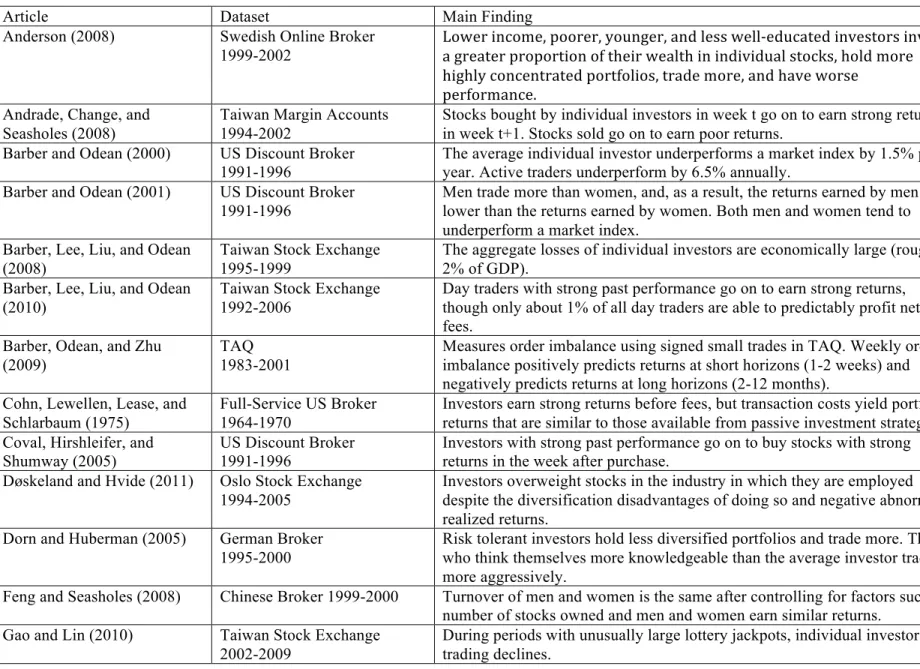
In this section, we provide an overview of evidence on the average performance of individual investors. In Table 1, we provide a brief summary of the articles we discuss. Collectively, the evidence indicates that the average individual investor underperforms the marketaboth before and after costs. However, this average (or aggregate) performance of individual investors masks tremendous variation in performance across individuals.
In research published through the late 1990s, the study of investor performance had focused almost exclusively on the performance of institutional investors, in general, and, more specifically, equity mutual funds.1 This was partially a result of data availability (there was relatively abundant data on mutual fund returns and no data on individual investors). In addition, researchers were searching for evidence of superior investors to test the central prediction of the efficient markets hypothesis: investors are unable to earn superior returns (at least after a reasonable accounting for opportunity and transaction costs).
While the study of institutional investor performance remains an active research area, several studies provide intriguing evidence that some institutions are able to earn superior returns. Grinblatt and Titman (1989) and Daniel, Grinblatt, Titman, and Wermers (DGTW, 1997) study the quarterly holdings of mutual funds. Grinblatt and Titman conclude (p.415) “superior performance may in fact exist” for some mutual funds. DGTW (1997) use a much larger sample and time period and document (p.1037) “as a group, the funds showed some selection ability.” In these studies, the stock selection
!!!!!!!!!!!!!!!!!!!!!!!!!!!!!!!!!!!!!!!!!!!!!!!!!!!!!!!!
1 A notable exception to this generalization is Schlarbaum, Lewellen, and Lease (1978), who analyze the round-trip trades in 3,000 accounts at a full-service US broker over the period 1964 to 1970. They document strong returns before trading costs, but after costs returns fail to match a passive index. One concern with these results is that the authors analyze the internal rate of return on round-trip trades, which biases their results toward positive performance since investors tend to sell winners and hold losers (the disposition effect). This dataset is also used in Cohn, Lewellen, Lease, and Schlarbaum, 1975; Lease, Lewellen, and Scharbaum, 1974; Lewellen, Lease, and Scharbaum, 1977.
! S! ability of fund managers generates strong before-fee returns, but is insufficient to cover the fees funds charge.2
In financial markets, there is an adding up constraint. For every buy, there is a sell. If one investor beats the market, someone else must underperform. Collectively, we must earn the market return before costs. The presence of exceptional investors dictates the need for subpar investors. With some notable exceptions, which we describe at the end of this section, the evidence indicates that individual investors are subpar investors.
To preview our conclusions, the aggregate (or average) performance of individual investors is poor. A big part of the performance penalty borne by individual investors can be traced to transaction costs (e.g., commissions and bid-ask spread). However, transaction costs are not the whole story. Individual investors also seem to lose money on their trades before costs.
The one caveat to this general finding is the intriguing evidence that stocks heavily bought by individuals over short horizons in the U.S. (e.g., a day or week) go on to earn strong returns in the subsequent week, while stocks heavily sold earn poor returns. It should be noted that the short-run return predictability and the poor performance of individual investors are easily reconciled, as the average holding period for individual investors is much longer than a few weeks. For example, Barber and Odean (2000) document that the annual turnover rate at a U.S. discount brokerage is about 75% annually, which translates into an average holding period of 16 months. (The average holding period for the stocks in a portfolio is equal to the reciprocal of the portfolios' turnover rate.) Thus, short-term gains easily could be offset by long-term losses, which is consistent with much of the evidence we summarize in this section (e.g., Barber, Odean, and Zhu (2009a)).
!!!!!!!!!!!!!!!!!!!!!!!!!!!!!!!!!!!!!!!!!!!!!!!!!!!!!!!!
2 See also Fama and French (2010), Kosowski, Timmerman, Wermers, and White (2006), and citations therein. Later in this paper, we discuss evidence from Grinblatt and Keloharju (2000) and Barber, Lee, Liu, and Odean (2009) that documents strong performance by institutions in Finland and Taiwan, respectively.
! @! It should be noted that all of the evidence we discuss in this section focuses on pre-tax returns. To our knowledge, there is no detailed evidence on the after-tax returns earned by individual investors because no existing dataset contains the account-level tax liabilities incurred on dividends and realized capital gains. Nonetheless, we observe that trading generally hurts performance. With some exceptions (e.g., trading to harvest capital losses), it is safe to assume that ceteris paribus investors who trade actively in taxable accounts will earn lower after-tax returns than buy-and-hold investors. Thus, when trading shortfalls can be traced to high turnover rates, it is likely that taxes will only exacerbate the performance penalty from trading.
1. 1. 1.Long-Horizon Results
Odean (1999) analyzes the trading records of 10,000 investors at a large discount broker over the period 1987-1993. Using a calendar-time approach, he finds that the stocks bought by individuals underperform the stocks sold by 23 basis points per month in the 12 months after the transaction (with p-values of approximately 0.07) and that this result persists even when trades more likely to have been made for liquidity, rebalancing, or tax purposes are excluded from the analysis. These results are provocative on two dimensions. First, this is the first evidence that there is a group of investors who systematically earn subpar returns before costs. These investors have perverse security selection ability. Second, individual investors seem to trade frequently in the face of poor performance.
Barber and Odean (2000) analyze the now widely used dataset of 78,000 investors at the same large discount brokerage firm (henceforth referred to as the LDB dataset). Unlike the earlier dataset, which contained only trading records, this dataset was augmented with positions and demographic data on the investors, and the analysis here focuses on positions rather than trades. The analysis of positions, from a larger sample of investors (78,000 v. 10,000) and a different time period (1991-1996 v. 1987-1993), provides compelling evidence that individual investors self-managed stock portfolios underperform the market largely because of trading costs.
! A! Barber and Odean (2000) sort households into quintiles based on their monthly turnover from 1991-1996. The total sample consists of about 65,000 investors, so each quintile represents about 13,000 households. The 20 % of investors who trade most actively earn an annual return net of trading costs of 11.4 %. Buy-and-hold investors (i.e., the 20 % who trade least actively) earn 18.5 % net of costs. The spread in returns is an economically large 7 percentage points per year.
These raw return results are confirmed with typical asset-pricing tests. Consider results based on the Fama-French three-factor model. After costs, the stock portfolio of the average individual investors earns a three-factor alpha of -31.1 basis points (bps) per month (-3.7 percentage points (pps) annually). Individuals who trade more perform even worse. The quintile of investors who trade most actively averages annual turnover of 258 %; these active investors churn their portfolios more than twice per year! They earn monthly three-factor alphas of -86.4 bps (-10.4 pps annually) after costs.
Grinblatt and Keloharju (2000) analyze two years of trading in Finland and provide supportive evidence regarding the poor gross returns earned by individual investors. The focus of their investigation is whether certain investors follow momentum or contrarian behavior with respect to past returns. In addition, they examine the performance of different categories of investors. Hampered by a short time-series of returns, they do not calculate the returns on portfolios that mimic the buying and selling behavior of investors. Instead, they calculate the buy ratio for a particular stock and investor category on day t, conditional on its future performance from day t+1 to day t+120, and test the null hypothesis that the buy ratio is equal for the top and bottom quartile of future performers. For households, the buy ratio for the top quartile is greater than the buy ratio for the bottom quartile on only 44.8% of days in the two-year sample period (p=0.08). For Finnish financial firms and foreigners, the difference in the ratios is positive on more than 55% of days. Individual investors are net buyers of stocks with weak future performance, while financial firms and foreigners are net buyers of stocks with strong future performance.
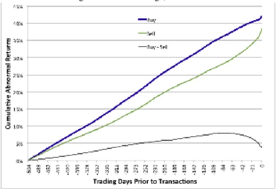
! G! Further confirmation regarding the perverse trading ability of individual investors comes from Taiwan. Barber, Lee, Liu, and Odean (2009) analyze the trading records of Taiwanese investors over the period 1995 to 1999. They construct portfolios that mimic the trading of individuals and institutions, respectively. When portfolios are constructed assuming holding periods that range from one day to six months, the stocks bought by institutions (sold by individuals) earn strong returns, while stocks bought by individuals (sold by institutions) perform poorly. A long-short strategy that mimics the buying and selling of individual investors and assumes a holding period of 140 trading days earns a negative abnormal return of 75 basis points per month before accounting for transaction costs (p<0.01).
The trading losses of individual investors in Taiwan are material. When one considers commissions and the transaction tax on sales, the aggregate trading losses of individuals are equal to 2.8% of total personal income in Taiwan and 2.2% of Taiwan’s total GDP. Back-of-the-envelope calculations indicate the net returns earned by individual investors in aggregate are 3.8 percentage points below market returns. Three factors contribute (roughly) equally to the shortfall: perverse stock selection ability, commissions, and the transaction tax, with a somewhat smaller role relegated to poor market timing choices.
The detailed trading information that we have on Finnish and Taiwanese investors is not available in the U.S. However, Hvidkjaer (2008) and Barber, Odean, and Zhu (BOZ, 2009a) use signed small trades from the TAQ database to infer the trading of individual investors in the U.S. The signing algorithm is a modified version of that proposed by Lee and Ready (1991), which identifies trades as buyer- or seller-initiated by comparing transaction prices to spreads. For each stock, both papers calculate a measure of order imbalance based on signed small trades (trades less than $5,000). BOZ verify that this is a reasonable measure of individual investor trading activity. Using the LDB dataset and a second dataset from a full-service broker (1997 to 1999) (hereafter the FSB dataset), BOZ document order imbalance calculated from signed small trades is highly correlated with order imbalance from retail trades at these two brokers. Specifically, the
! b! correlation between order imbalance based on small trades in TAQ and order imbalance from the broker trading records is about 50%. In contrast, the correlation between order imbalance based on large trades (trades over $50,000) and broker trading records is reliably negative. This evidence indicates that small trades are a good proxy for the behavior of individual investors during this period.3
Using small trades as a proxy for the trading of individual investors, both Hvidkjaer (2008) and BOZ (2009a) document that stocks heavily bought by individuals over horizons ranging from one month to one year go on to underperform stocks heavily sold by individuals. For example, Hvidkjaer sorts stocks into deciles based on signed small trade turnover (i.e., buys less sells divided by shares outstanding). At a formation period of six months, the top decile (stocks heavily bought) underperforms the bottom decile (stocks heavily sold) by 89 basis points per month (p<0.01).
1. 1. 2.Short-Horizon Results
Contrary to the long-run evidence discussed above, the returns earned by individual investors over short horizons (up to a week) appear to be quite strong. Kaniel, Saar, and Titman (KST, 2008) document individual investor trading positively predicts short run returns. KST identify individual investor trades using the 2000 to 2003 NYSE’s Consolidated Audit Trail Data (CAUD) files, which contains detailed information on all orders that execute on the exchange, including a field that identifies whether the order comes from an individual investor. Measuring order imbalance over a nine-week horizon, they document the top decile of stocks heavily bought by individuals earn market-adjusted returns of 16 bps over the next 20 trading days (about a month), while the bottom decile (i.e., stocks heavily sold) earn -33 bps. KST argue that their results are largely consistent with individual investors acting as “…liquidity providers to institutions that require immediacyc!(p.274). Analyzing the same data, Kaniel, Liu, Saar, and Titman (2011) find evidence consistent with informed trading by individual investors around !!!!!!!!!!!!!!!!!!!!!!!!!!!!!!!!!!!!!!!!!!!!!!!!!!!!!!!!
3 Given the adoption of price decimalization in 2001 and the spread of algorithmic trading, the proportion of volume traced to small trades has increased dramatically. We suspect these developments undermine the use of small trades as a proxy for the behavior of individual investors post-2001. O’Hara, Yao, and Ye (2011) confirm our suspicions.
! ?! earnings announcements. They document that the stocks bought in aggregate by individuals in the 10 days prior to an earnings announcement outperform those sold in aggregate by about 1.5% in the two days around the earnings announcement. They argue liquidity provision and private information contribute equally to the strong returns earned by individuals around earnings announcements.
Similarly, BOZ (2009) document that small trade order imbalance from TAQ positively predicts returns over short horizons. Specifically, when order imbalance is measured at a weekly horizon, stocks heavily bought outperform for the subsequent two weeks before going on to underperform for the remainder of the year. It is difficult to attribute these patterns to liquidity provision as the order imbalance in BOZ is based on signed rather than all trades. If a stock is bought at a price above the quoted spread, it is categorized as a buy, while if the stock is sold at a price below the quoted spread, it is categorized as a sell. This signing yields order imbalance measures that are based only on liquidity demanders rather than on liquidity suppliers, presenting a challenge for the KST liquidity provision story. Indeed the contemporaneous relation between returns and order imbalance is positive in BOZ (what one would expect when order imbalance is based on liquidity demanders), but negative in KST (what one would expect when order imbalance is based on liquidity providers). BOZ argue that the combination of a positive relation between small trade order imbalance and short-horizon returns, followed by return reversals at long horizons, can be explained by the correlated sentiment-based trading of individual investors. In the short run, sentiment temporarily pushes prices above fundamental value, leading to predictable long-run return reversals.
Kelley and Tetlock (KT, 2011) use data routed by retail brokers to two market centers over the period 2003 to 2007 to analyze the trading of individual investors. Brokerage firms route a significant fraction of their order flow (roughly 40%) to these market centers, and the data contain a code that classifies the order submitter as an individual or institution. Using a daily Fama-Macbeth regression approach, KT document that daily order imbalance of retail traders positively predicts returns at horizons up to 20 days. KT (2010) argue the strong returns over short horizons is evident in both market
! BE! and limit orders. They conclude “…retail market orders aggregate private information about firms’ future cash flows, whereas retail limit orders provide liquidity to traders demanding immediate execution.”
These four papers use somewhat different approaches, datasets, and time periods. All four present intriguing evidence that individual investors’ trades positively predict returns at short horizons in the U.S. There is an ongoing debate in the literature regarding the origins of this short-run predictability in the U.S.
In contrast to the consistent finding of short-run predictability in the U.S., the non-U.S. evidence is mixed. Barber, Lee, Liu, and Odean (2009) document that individual investors in Taiwan incur losses over short horizons. Long-short portfolios that mimic the buy-sell trades of individual investors earn reliably negative monthly alphas of -11.0%, -3.3%, and -1.9% over horizons of 1, 10, and 25 days respectively. Andrade, Chang, and Seasholes (2008) document a similar result using changes in stocks held in margin accounts by individual investors in Taiwan over the period 1994 to 2002. In Andrade et al., stocks are sorted into quintiles based on their order imbalance in week t; stocks heavily bought go on to earn poor returns (-23 bps) in the following week, while those heavily sold earn strong returns (29 bps). Kaniel, Saar, and Titman (2008) speculate that their liquidity provision story does not apply to the Taiwan market, where individual investors dominate trading; roughly 90% of total trading volume can be traced to retail investors in Taiwan.
1. 1. 3.Market v. Limit Orders
The evidence on the profitability of market v. limit orders of individual investors also yields conflicting results. Kelley and Tetlock (2011), which we discussed in the prior section, document short-term profits on retail trades emanating from both market and limit orders in the U.S. Linnainmaa (2010) documents losses on limit orders and gains on market orders in Finland. Barber, Lee, Liu, and Odean (2009) find the opposite result in Taiwanashort-term gains on passive orders and short-term losses on aggressive (quasi-market) orders.
! BB! Linnainmaa (2010) argues that individual investors perform poorly on their trades because informed traders pick off their limit orders. Assume sleepy individual investors have unmonitored limit orders to sell a stock. A savvy investor learns of a good earnings announcement that will drive the stock’s price higher. Armed with this earnings news, the savvy investor places market orders to buy the stock and profits in the short-term by picking off the unmonitored limit orders of individual investors. Linnainmaa (2010) uses data from the Finnish Stock Exchange over the period 1998 to 2001 that allows him to identify whether an investor has placed a limit or market order. Consistent with the hypothesis that individual investors are picked off, he documents that the returns on individual investor trades that emanate from limit orders lose 51 bps on the day following trade and 3.3% over 63 days. In contrast, the returns on trades that emanate from market orders gain 44 bps on the day following trade and 3.5% over 63 days. In Finland, individual investors lose money on executed limit orders, but make money on executed market orders. When combined, the gains and losses leave individual investors in his sample with profits that are indistinguishable from zero.
The evidence from Taiwan is not consistent with that from Finland. Taiwan is an electronic limit order market. Barber, Lee, Liu, and Odean (2009) categorize the limit orders as passive or aggressive. Orders to buy with prices in excess of the most recent unfilled sell limit order are categorized as aggressive; those with an order price below the most recent unfilled buy limit order are categorized as passive. (Sell orders are categorized as passive or aggressive in a similar way.) One can view aggressive limit orders as roughly equivalent to market orders since the only way to demand execution in an electronic limit order market is to place an order with an aggressive price (e.g., be willing to buy at a high price or sell at a low price). At short horizons (of one to 10 days following the trade), individual investors make money on their passive trades, though the six-month returns are indistinguishable from zero. Individual investors lose money on their aggressive trades at both short and long horizons. This is in striking contrast to the results in Finland, where individuals lose money on limit orders and make money on market orders.
! BH!
1.2. Cross-Sectional Variation in Performance
The performance of the average individual obscures tremendous variation in outcomes across individuals. Importantly, the cross-sectional variation in performance is predictable and can be traced to investment skill, cognitive abilities, investment style, location, and gender.
There is strong evidence of performance persistence among individual investors. Coval, Hirshleifer, and Shumway (CHS, 2005) use the LDB dataset to analyze performance persistence: Do investors with strong past returns go on to earn strong returns? They sort investors into deciles based on the performance of their buys during the first half of the sample period (1991 to 1993) and analyze the subsequent performance of their purchases in the second half of the sample period (1994 to 1996). Using buys during the latter period, CHS construct a calendar-time portfolio that mimics the buying of investors in each performance decile. The return spread between the top and bottom performance deciles is about 5 bps per day in the week following trade. This return spread does not account for transaction costs; round-trip spreads and commissions would easily wipe out a 25 bps trading advantage. Nonetheless, the evidence of variation in investor skill is intriguing.
Barber, Lee, Liu, and Odean (2011) analyze the performance of day traders in Taiwan over the period 1992 to 2006. Day trading in Taiwan is quite common. Over 300,000 individual investors engage in day trading in the typical year, and their combined trading accounts for 17% of total trading volume. This is an ideal setting to analyze the performance of speculators, as day traders are certainly not trading for liquidity, rebalancing, or tax-related reasons (all reasonable motivations for trading). Furthermore, the large population of day traders allows for a more powerful identification of potentially skilled traders. To identify skilled (and unskilled) traders, BLLO (2011) rank investors based on their day trading performance in year y and analyze their performance in the subsequent year (y+1). The top 500 traders earn intraday returns on day trading that outperform the thousands of traders who perform poorly by over 60 basis points. As in
! BD! CHS, there is strong evidence of cross-sectional differences in speculative ability though the magnitudes are much larger. The best traders, though a rare breed, earn gross abnormal returns of about 50 bps per day, which is sufficient to cover a reasonable accounting for transaction costs.
Recent papers suggest cognitive abilities play an important role in investor outcomes. Korniotis and Kumar (2009a) predict cognitive ability using a host of demographic variables (e.g., age, education, and social networks). Using the LDB dataset, they show that smarter investors outperform others by about 30 bps per month (or 3.6% annually) both before and after accounting for transaction costs. Smarter investors earn returns net of trading costs that are on par with appropriate benchmark returns; they make good stock picks, but only good enough to cover their trading costs. Other investors underperform appropriate benchmarks by a bit more than 30 basis points per month (or 3.6% annually) after costs, with about half of the shortfall being traced to trading costs and half to bad stock selection.
In a closely related paper, Korniotis and Kumar (2009b) use the LDB dataset to analyze the relation between age and performance. Motivated by the observation that cognitive abilities decline with age, the authors predict and find evidence to support the notion that investment performance declines with age.
Using data from Finland, Grinblatt, Keloharju, and Linnainmaa (GKL, 2010) analyze the relation between IQ and stock selection ability. The Finnish Armed Forces administers an intelligence test (120 questions covering verbal, math, and logical reasoning) to recruits around the time of induction into mandatory military duty (generally at the age of 19 or 20). The scores range from 1 to 9, and GKL define a low IQ investor as one with a FAF score from 1 to 4 and a high IQ investor as one with a FAF score of 9. Based on these definitions, 24% of their sample are low IQ investors, while 8% are high IQ investors. The spread in portfolio returns earned by low- versus high-IQ investors is 2.2% per year and is marginally significant. However, an analysis of the returns following purchases provides convincing statistical evidence that high-IQ
! BS! investors make better trades than low-IQ investors. GKL also document high-IQ investors have better trade execution, though they do not measure the net portfolio returns of high-IQ investors, so it is difficult to know whether high-IQ investors would beat an appropriate benchmark after a reasonable accounting for transaction costs.
Ivkovic, Sialm, and Wiesbenner (2008) argue that informed individual investors would tend to concentrate their portfolios in the stocks for which they hold an informational advantage. Using the LDB dataset, they document that investors with concentrated portfolios (with only one or two stocks) outperform diversified portfolios (with three or more stocks) by 16 bps per month. This “concentration” effect is more pronounced for local stock and non-S&P 500 stocks.
Finally, Barber and Odean (2001) compare the performance of men and women using data from the LDB dataset. Unlike the studies on cross-sectional performance discussed above, this study focuses on the net returns (i.e., returns net of spreads and commissions) of men and women. The study is motivated by the two observations: (1) men tend to be more prone to overconfidence than women in areas culturally perceived to be in the male domain (Deaux and Farris, 1977), and (2) models that assume investors are overconfident tend to predict investors will trade excessively and to their detriment. When combined, these observations predict that men will trade more than women and that excessive trading will hurt their performance. Consistent with these predictions, Barber and Odean (2001) document that men trade more than women; the annual turnover rates of men are about 80%, while those of women are 50%. The excessive trading of men leads to poor returns. While both men and women earn poor returns, men perform worse. Virtually all of the gender-based difference in performance can be traced to the fact that men tend to trade more aggressively than women. Neither men nor women appear to have stock selection ability (i.e., the gross returns earned on their trades are similar), so men’s tendency to trade aggressively and the resulting trading costs drag down men’s returns. Dorn and Huberman (2005) find that men with accounts at a German online brokerage trade more actively than women, but gender effects are reduced if one accounts for differences in self-reported risk-aversion. Choi, Laibson, and Metrick,
! B@! 2002, Agnew, Balduzzi, and Sundén, 2003, and Mitchell, Mottola, Utkus, and Yamaguchi, 2006, all report that while trading levels are low in 401(k) plans, men trade more actively than women. In contrast to the U.S. and German and 401(k) plan evidence, Feng and Seasholes (2008) find no significant turnover or performance differences in the accounts of men and women in China.
>!.$#)2+1!#)$%734!02!,/)!#)9)$#./!03!.#099I9).,703$1!8$#7$,703!73!T)#20#5$3.)! :7)1%9! ,/#))! 4)3)#$1! .03.1+97039'! ! `7#9,<! ,/)#)! 79! 9,#034! )87%)3.)! 02! .#099I9).,703$1! 8$#7$,703!73!,#$%734!9R711'!-).03%<!9).+#7,:!9)1).,703!9R711!$5034!73%787%+$19!79!#$#)! C7')'<! .03273)%! ,0! $! #)1$,78)1:! 95$11! 4#0+T! 02! 9,0.R9! 0#! 73%787%+$19F'! N/7#%<! )8)3! ,/)! ()9,!9,0.R!T7.R)#9!/$8)!,#0+(1)!.08)#734!,#$39$.,703!.09,9'!
2.
Why do Individual Investors Underperform?
The majority of the empirical evidence indicates that individual investors, in aggregate, earn poor long-run returns and would be better off had they invested in a low-cost index fund. This evidence of poor performance is particularly compelling when we include transaction costs (e.g., commissions, bid-ask spreads, market impact, and transaction taxes). While transaction costs are an important component of the shortfall, a second component is the poor security selection ability of individual investors documented in many studies that we reviewed in the prior section. These observations lead one to wonder why investors trade so much and to their detriment.
2.1. Asymmetric Information
One possibility is that individual investors realize that they are at an informational disadvantage when trading and only do so for non-speculative reasons including liquidity needs, rebalancing, and taxes. Investors may need to purchase stocks to save or sell stocks to consume. At times, investors may need to rebalance their portfolios to manage risk-return tradeoffs. Occasionally, investors will want to harvest tax losses to minimize their tax bill. When faced with these liquidity, rebalancing, or tax management needs, retail investors are forced to trade with others who might be better informed. It is, however, difficult to reconcile non-speculative trading needs with the annual turnover
! BA! rates of 250 % for the 20 % most active investors in the LDB dataset (Barber and Odean 2000), annual turnover of 300 % in Taiwan (Barber, Lee, Liu, and Odean, 2009), or annual turnover of 500 % in China (Gao, 2002). Furthermore, investors who do have unusual non-speculative needs to trade could dramatically lower their asymmetric information and transaction costs by investing in low cost, no load mutual funds.
Why do so many investors self-manage portfolios when they could earn better returns with lower risk in low-cost mutual funds, such as index funds? And why do investors with portfolios of individual equities trade actively when doing so lowers their expected returns? We turn to possible behavioral explanations.
2.2. Overconfidence!
Overconfidence can explain the relatively high turnover rates and poor performance of individual investors. A rich literature in psychology documents that people generally are overconfident (for an overview of this literature see Moore and Healy (2008) and citations in Odean (1999)). One variety of overconfidence is a belief that one knows more than one actually does, which is sometimes labeled “miscalibration” or “overprecision.” In a classic illustration of this type of overconfidence, subjects are presented a series of 10 difficult questions (e.g., “What is the length of the Nile river?”). They are then asked to provide a low and high guess such that the correct answer is between the low and high guess with a probability of 90 %. The well-calibrated subject would, on average, provide intervals that contain the correct answer nine out of 10 times. Typically, subjects provide intervals that contain far fewer correct answers (Alpert and Raiffa (1982)). A second variety of overconfidence is a belief that one is better than the median person, which has been (mis)labeled the “better-than-average” effect. For example, when asked about their own driving ability relative to the population of drivers, most people rank themselves above the driver of median ability (Svenson (1981)). Related to, but distinct from, the better-than-average effect is the tendency to overestimate one’s actual ability. For example, a student might think his score on a test is 80% when he actually scored 65% (and the average score was 90%). (See Moore and Healy (2008) for discussion.)
! BG! Several papers have developed theoretical models based on the observation that investors are overconfident (Benos (1998), Caballe and Sakovics (2003), Daniel, Hirshleifer, and Subrahmanyam (1998), Gervais and Odean (2001), Hong, Scheinkman, and Xiong (2006), Kyle and Wang (1997), Odean (1998), Peng and Xiong (2006), Scheinkman and Xiong (2003), and Wang (2001)). Generally, these models assume investors suffer from the miscalibration type of overconfidence. For example, one can extend the classic models of Kyle (1985), Grossman and Stiglitz (1980), or Diamond and Varecchia (1981) by assuming some investors are miscalibrated (or overconfident) about the precision of their information (see Odean (1999)). In these three settings, the overconfidence models generally predict that investors will trade too much and to their detriment.
A number of empirical facts line up reasonably well with the predictions of these theoretical models. Investors who trade the most perform the worst (Barber and Odean (2000)). Men, who are more prone to be overconfident than women, trade more and perform worse than women (Barber and Odean (2001)).
Empirical work has attempted to tease out the type of overconfidence, miscalibration or better-than-average, that is linked to excessive trading. Combining survey evidence with trades and positions for 1,345 German investors, Dorn and Huberman (2005) document that investors who think themselves more knowledgeable than average churn their portfolios more. Similarly, Glaser and Weber (2007) use survey evidence and trading records for 215 German investors to document a link between the “better-than-average” type of overconfidence and trading activity. Using a five-question version of the calibration experiment described earlier, Glaser and Weber find no reliable link between the miscalibration type of overconfidence and trading activity. (While this is a provocative nonresult, using a five- or 10-question survey to measure miscalibration strikes us as a very noisy measure that would yield low power to reject the null hypothesis that miscalibration and trading activity are unrelated.) Finally, Grinblatt and Keloharju (2009) find that Finnish investors with an inflated sense of their own abilities tend to trade more; we elaborate on this finding in more detail in the next section.
! Bb! Closely related to the notion of overconfidence are self-assessments of competence, which are studied by Graham, Harvey, and Huang (2009). They argue that “people are more willing to bet on their own judgments when they feel skillful or knowledgeable.” To test this conjecture, they use survey responses from 475 U.S. investors to study the impact of self-assessed competence on trading. Competence is based on the answer to the following question “How comfortable do you feel about your ability to understand investment products, alternatives, and opportunities?” Subjects responded on a five-point scale ranging from “1-very uncomfortable” to “5-very comfortable.” Graham et al. document a strong link between self-assessed competence and the propensity to trade. They measure the better-than-average effect by taking the difference between the answers to questions about an investor’s expected return on their own portfolio and the expected return on the market. They find weak evidence that this measure of overconfidence is linked to trading activity.
In summary, a fair amount of evidence indicates that the better-than-average and overestimation varieties of overconfidence are correlated with higher levels of trading by investors. While the evidence that miscalibration is linked to trading is weaker, we suspect this weak link might be partially explained by the current inability to measure miscalibration well.
2.3. Sensation Seeking
A noncompeting explanation for the excessive trading of individual investors is the simple observation that trading is entertainment and appeals to people who enjoy sensation-seeking activities such as gambling. Using the Finnish dataset, Grinblatt and Keloharju (GK, 2009) analyze both sensation-seeking and overconfidence as mechanisms that lead to trading. They use traffic tickets as a proxy for sensation-seeking and argue that those who speed are more likely to be sensation seekers. To measure overconfidence, GK use data from tests administered to men entering the Finnish Armed Forces that measure the candidates’ actual ability (i.e., test outcomes) and perceived ability (i.e., self-assessments). GK use the measure of perceived ability that is orthogonal to actual ability as a measure of overconfidence. Using these instruments, GK document that both
! B?! sensation-seeking and overconfidence affect trading, though the tenor of their results depend a bit on whether one focuses on the decision to trade, the number of trades, or portfolio turnover as the dependent variable of interest.
Dorn and Sengmueller (2009) marry survey responses and trading records for 1,000 investors at a German discount broker. Investors are asked whether they agree or disagree (on a five-point scale) with the following four statements: (1) I enjoy investing, (2) I enjoy risky propositions, (3) Games are only fun when money is involved, and (4) In gambling, the fascination increases with the size of the bet. Investors who agree with these statements tend to trade more. Investors who report enjoying investing (question 1) or gambling (questions 2-4) trade at twice the rate of other investors.
Trading competes with other activities for the attention of sensation-seeking investors. Thus, we would expect trading to wane when there are a number of thrilling activities at their disposal. There is some suggestive evidence that this is the case. Dorn, Dorn, and Sengmueller (2007) analyze the trading response of individual investors to multi-state lottery jackpots in the U.S. Using small trades in the TAQ dataset to identify individual investors during the period 1998 to 2004, they document that a one standard deviation increase in multistate lottery jackpots (i.e., Powerball and Mega-Millions) is associated with a 1% reduction in small trader participation (the fraction of trading volume contributed by trades of less than $5,000); this effect is most pronounced for lottery-like stocks (e.g., low-prices stocks with high past volatility and skewness). Similarly, Barber, Lee, Liu, and Odean (2009) find that trading in Taiwan drops by about 25% when a legal lottery was introduced on the island in April 2002. As in Dorn, Dorn, and Sengmueller (2007), Gao and Lin (2010) further explore this substitution effect by analyzing the volume of individual investor trading in Taiwan around lotteries with unusually large jackpots. They document trading by individual investors declines during periods with unusually large lottery jackpots; moreover, the effects are greatest in stocks with high levels of individual investors participation and skewed returns.
! HE! In related papers, Kumar (2009b) and Mitton and Vorkink (2007) hypothesize that retail investors have a taste for stocks with lottery-like payoffs. Note that this is distinct from the sensation-seeking (or entertainment) hypothesis discussed above. Sensation-seeking investors will trade to entertain themselves but might hold well-diversified portfolios and eschew lottery-like stocks. Investors with a preference for skewness will hold lottery-like stocks but might refrain from trading. Thus, preferences for skewness may lead to underdiversification but has no immediate implications for trading. We elaborate on these findings later when we discuss the literature on diversification.!!
2.4. Familiarity
There is debate about whether individual investors possess an informational advantage about companies that are close to where they live or in their industry of employment. Some scholars argue that individual investors are better informed about the prospects of companies close to where they live or in their industry of employment and that this information advantage leads to superior investment performance. Others argue individuals overinvest in these stocks because they are familiar to them, leading to underdiversification and average or even below-par returns. In this section, we discuss the evidence on performance. In section VI, we discuss the implications for diversification.
Massa and Simonov (2006) analyze portfolio holdings of Swedish investors and document that investors tilt their portfolio towards stocks that are most closely related to them, either professionally (e.g., a financial professional investing in a finance stock) or geographically (e.g., a Seattle investor investing in a Seattle stock). They argue that this familiarity-based investing allows investors to earn higher returns because of the information advantage conferred by familiarity. Similarly, Ivkovic and Weisbenner (2005) use the LDB dataset to document individual investors tend to overweight local stocks and argue the returns on local stocks are strong. Seasholes and Zhu (2010) argue that this result is not robust and leans on faulty statistical methodologies. After considering a battery of tests using the same dataset as Ivkovic and Weisbenner (2005), they conclude that individual investors do not earn superior returns on local stocks. Døskeland and Hvide (2011) document that, after excluding own-company stock
! HB! holdings, individual investors in Norway overweight stocks in the industry in which they are employed despite the diversification disadvantages of doing so and earn negative abnormal returns on the stocks they buy in their industry of employment.
In summary, the performance implication of investing in geographically or occupationally familiar stocks is the subject of ongoing debate. However, investors overweight these stocks in their equity portfolios, which has potentially important implications for diversification, a subject we return to later in this review.
!
3.
The Disposition Effect: Selling Winners and Holding Losers
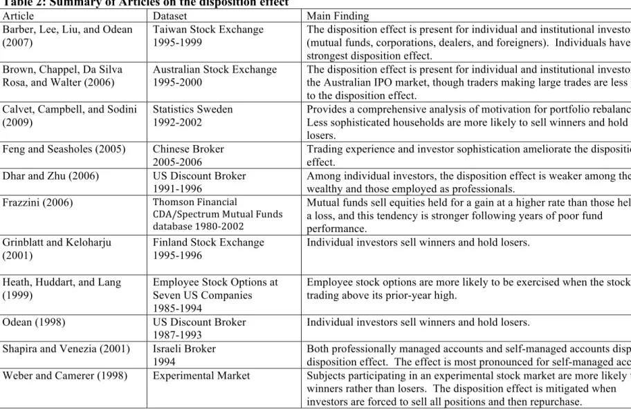
Individual investors have a strong preference for selling stocks that have increased in value since bought (winners) relative to stocks that have decreased in value since bought (losers). Shefrin and Statman (1985) labeled this behavior the “disposition effect”—investors are disposed to sell winners and hold losers. In this section, we begin by illustrating the basic effect. We then survey the empirical and experimental work documenting the disposition effect, which we summarize in Table 2. We close by discussing possible explanations for the disposition effect.
3.1. The Evidence
The disposition effect is a remarkably consistent and robust phenomenon. Before diving into the literature on this topic, we illustrate the basic effect using data from the LDB dataset and the Finnish dataset from 1995 to 2008. (The analysis of the Finnish dataset was provided to us by Noah Stoffman.) Specifically, we estimate models of the form
where h(t,x(t)) is the hazard rate at time t conditional on a set of p observed predictors as of period t (denoted x(t)). The baseline hazard rate, h0(t), is the hazard rate when all predictors take on a value of zero. The ! coefficients are estimated from the data. The hazard rate is the probability density function of the hazard event at time t conditional on survival to time t (i.e., not observing the hazard event prior to t).
!
! HH! In our analyses, the hazard event is the sale of a stock, and time is measured in days subsequent to the original purchase. The hazard rate for a particular stock being sold by a particular investor is conditional on the covariates for that stock and investor at time t.
For each kth covariate, we report estimates of the hazard ratio assuming a one-unit increase in the covariate:
Note that the hazard ratio, exp(!k), is the ratio of hazard rates for two stocks with the
same covariates except that xk is one unit larger for the stock whose hazard rate is given in the numerator. Thus, if xk is a dummy variable, the hazard ratio is the ratio of the hazard when the dummy variable takes on a value of 1 to the hazard when its value is 0 and all other covariates are the same.
The Cox model makes no assumptions about how the baseline hazard rate changes over time and does not estimate the baseline hazard rate. The model does assume that hazard ratios do not change with time. For example, the model makes no assumptions about how the unconditional rate of selling stocks changes from day 50 to day 100, but the model does assume that if a winner is sold at a 20% higher rate than a loser on day 50, then the winner will also be sold at a 20% higher rate than a loser on day 100.
To analyze how the magnitude of the return since a stock was purchased affects the hazard rate of selling the stock, we create dummy variables for 4% wide return categories. These return categories are:
r " -42%, -42% < r " -38%, …, -2% < r " 2%, …, 58% < r " 62%, 62% < r.
For example, we create a dummy variable that is one if the return at the time of the sale is greater than -2% and less than or equal to 2%. These covariates are time varying since the return since purchase can change daily.
!
exp("k)=
h0(t)exp("1x1+...+"k(xk+1)+...+"pxp) h0(t)exp("1x1+...+"kxk+...+"pxp)
! HD! For the LDB dataset, we estimate one model for the full sample period (1991 to 1996) and base confidence intervals on the estimated standard errors for the single model. For the Finnish dataset, separate models are estimated for each sample year (1995 to 2008) and then the results are averaged across years. Confidence intervals are based on the time-series standard errors of coefficient estimates (i.e., an adaptation of the Fama-Macbeth approach to calculating standard errors that assumes serial independence in the estimated coefficients).4
In Figure 1, Panel A, we plot the hazard ratio for selling (y axis) for various levels of return since the stock was purchased (x axis) using data from the large discount brokerage covering the period 1991 to 1996. In Panel B, results using the Finnish data are plotted. The general patterns of the hazard ratios are remarkably consistent.
Consider the large discount broker (Panel A). The default hazard rate is the omitted return category that includes returns of -2% to 2%. The tendency to sell a stock increases dramatically as returns increase. For example, the hazard rate for selling stocks up between 18-22% since purchased is 2.65 times greater than the hazard rate for selling stocks that have experienced returns between -2% and 2%. Negative returns since a stock was purchased also increase the hazard rate of selling, but not as dramatically as positive returns. For example, the hazard rate for selling stocks up 18-22% since purchased is 1.77 times greater than the hazard rate for selling stocks down 18-22% since purchased. The results are qualitatively similar for the Finnish data.
A number of studies—both experimental and empirical—confirm the presence of the disposition effect. Weber and Camerer (1998) provide early experimental support for the disposition effect. In their experiment, subjects observe price changes on six stocks (stocks A to G) over 14 periods. The probability that a stock will increase in value varies across stocks, but not rounds. Subjects know the distribution of these probabilities, but do not know which stock has the highest probability of increasing in price. A rational !!!!!!!!!!!!!!!!!!!!!!!!!!!!!!!!!!!!!!!!!!!!!!!!!!!!!!!!
4 Since the Cox models are computationally intense with time-varying covariates (i.e., returns since purchase) and many households, estimating one model for the full 1995 to 2008 sample period is computationally challenging.
! HS! Bayesian would conclude that the stock with the most price increases has the greatest chance of being the stock with a high probability of further increasing in value, so the disposition effect (selling winners, holding losers) is clearly counterproductive in this setting. Nonetheless, subjects sell winners at 50% higher rate than losers; 60% of sales are winners, while 40% of sales are losers.
Odean (1998) examines trading records for 10,000 accounts at a large U.S. discount brokerage for the period 1987 through 1993. In brief, Odean compares the rate at which investors sell winners (realized gains) and losers (realized losses) and compares the realization of gains and losses to the opportunities to sell winners and losers. He finds that, relative to opportunities, investors realize their gains at about a 50% higher rate than their losses and that this difference is not explained by informed trading, a rational belief in mean-reversion, transactions costs, or rebalancing. (See Calvet, Campbell, and Sodini (2009) for a comprehensive analysis of the rebalancing of household portfolios.)
Grinblatt and Keloharju (2001a) examine the disposition effect using the trading records for virtually all Finnish investors during 1995 and 1996. Controlling for a wide variety of factors, they find that investors have a tendency to hold onto losers. Relative to a stock with a capital gain, a stock with a capital loss of up to 30% is 21% less likely to be sold; a stock with a capital loss in excess of 30% is 32% less likely to be sold. Furthermore, stocks with high past returns or trading near their monthly high are more likely to be sold.
Heath, Huddart, and Lang (1999) find that employee stock options are more likely to be exercised when the stock is trading above its previous year’s high and that exercise is positively related to stock returns during the previous month and negatively related to returns over longer horizons.
Kaustia (2004) tracks trading volume following IPOs and finds that IPOs that opened below their offer price experience significantly more trading volume when they
! H@! trade above rather than below the offer price. Brown, Chappel, da Silva Rosa, and Walter (2006) analyze records for Australian investors who subscribed to IPOs between 1995 and 2000 and find that the disposition effect “… is pervasive across investor classes.”
The disposition effect has been documented for individual investors in several countries, for some groups of professional investors, and for different types of assets. Shapira and Venezia (2001) analyze the trading of 4,330 investors with accounts at an Israeli brokerage in 1994. About 60% of these accounts are professionally managed,
while for other accounts, investors make independent decisions. They measure the
duration of round-trip trades conditional on whether the stock was sold for a gain or loss. A tendency to sell winners and hold losers would, ceteris paribus, yield shorter holding periods for winners v. losers. Both professionally managed accounts and independent accounts exhibit the disposition effect (the holding periods for winners is roughly half that of losers), though the effect is somewhat stronger for independent accounts.
Feng and Seasholes (2005) use hazard rate models to estimate the magnitude of the disposition effect for 1,511 Chinese investors using trades data from a Chinese broker in 2000. These Chinese investors are 32% less likely to realize a loss. Chen, Kim, Nofsinger, and Rui (2007) analyze almost 50,000 Chinese investors using data from a Chinese brokerage firm over the period 1998 to 2002. Using methods similar to those in Odean (1998), Chen et al. document that Chinese investors are 67% more likely to sell a winner than a loser. For a small subsample of 212 institutional investors who trade through this broker, Chen et al. document a much weaker disposition effect as institutions are only 15% more likely to see a winner. Choe and Eom (2009) find a disposition effect for investors in Korean stock index futures; the effect is strongest for individual investors. Compelling evidence beyond Chen et al. (2007) and Choe and Eom (2009) suggests that institutions suffer from the disposition effect, albeit to a lesser extent than individual investors. Frazzini (2006) estimates, from 1980 through 2002, the rates at which U.S. mutual funds realize gains and losses in their equity holdings relative to how many positions they hold for a gain or a loss. For all funds, gains are realized at a rate 21%
! HA! higher than losses; for funds in the previous year’s bottom performance quintile, gains are realized at a rate 72% higher than losses. Barber, Lee, Liu, and Odean (2007) analyze trading records for all investors at the Taiwan Stock Exchange from 1995 to 1999 to compare the disposition effect of individual and various categories of institutional investors. They find a strong disposition effect for individual investors, who are nearly four times as likely to sell a winner rather than a loser. Corporate investors and dealers also are disposed to selling winners (though the effect is much weaker than that observed for individuals), but neither Taiwan mutual funds nor foreign investors in Taiwan are disposed to selling winners.
Consistent with this investment behavior being a mistake that has its origins in cognitive ability or financial literacy, the disposition effect is most pronounced for financially unsophisticated investors. For example, the disposition effect tends to be stronger for individual rather than institutional investors (Brown et al. (2006), Chen et al. (2007), Choe and Eom (2009), and Barber et al. (2007)). Dhar and Zhu (2006) use the LDB dataset to document that wealthier and professionally-occupied investors are less likely to sell winners and more likely to sell losers. Calvet, Campbell and Sodini (2009) document a similar result among Swedish investors. Finally, in the LDB data, investors who place more trades on the same day are less likely to exhibit the disposition effect (Kumar and Lim (2008)) and the disposition effect is greatest for hard-to-value stocks (Kumar (2009a)).
There is also intriguing evidence that investors learn to avoid the disposition effect over time. Among the Chinese individual investors they study, Feng and Seasholes (2005) document that the disposition effect dissipates with trading experience (time since first trade) and various measures of financial sophistication measured early in a trader’s history. Seru, Shumway, and Stoffman (2010) examine trading records for individual investors in Finland from 1995-2003. They find that the disposition effect declines with experience when experience is measured in number of trades. The drop in the disposition effect is much less when trading experience is measured in years.
! HG! The research discussed above presents a remarkably clear portrait of a prototypical individual investor who sells his winners and holds his losers. This behavior is broadly categorized as an investment mistake because it is tax inefficient.5 Thus, while taxes clearly affect the trading of individual investors, they cannot explain the disposition effect. Investors' reluctance to realize losses is at odds with optimal tax-loss selling for taxable investments. For tax purposes, investors should postpone taxable gains by continuing to hold their profitable investments. They should capture tax losses by selling their losing investments, though not necessarily at a constant rate. Constantinides (1984) shows that when there are transactions costs, and no distinction is made between the short-term and long-term tax rates, investors should increase their tax-loss selling gradually from January to December.6 Australia has a June tax year end, so the Constantinides model would predict accelerated selling in June for Australia, a prediction confirmed by Brown et al. (2006).
Barber and Odean (2004) document the disposition effect for taxable and tax-deferred accounts for the LDB dataset and for a dataset of trading and position records from January 1998 through June 1999 for 418,332 households with accounts at a large U.S. full-service brokerage. They find that at both the discount and full-service brokers, the disposition effect is reversed in December in taxable, but not tax-deferred, accounts. Using a Cox proportional hazard rate model and the U.S. discount brokerage data, Ivkovich, Poterba, and Weisbenner (2005) document that “Investors are more likely to realize losses in taxable accounts than in tax-deferred accounts, not just in December, but throughout the year.”
3.2. Why do investors prefer to sell winners?
While the tendency of investors to sell winners more readily than losers is empirically robust, recent research focuses on why investors behave this way. Shefrin and Statman (1985) attribute the disposition effect to a combination of prospect theory, regret aversion, mental accounting, and self-control issues. Prospect theory was developed from !!!!!!!!!!!!!!!!!!!!!!!!!!!!!!!!!!!!!!!!!!!!!!!!!!!!!!!!
5 In addition, selling winners rather losers arguably leaves individual investors missing out on some returns that might be earned because of momentum effects (Jegadeesh and Titman (1991)).
6 Dyl (1977), Lakonishok and Smidt (1986), and Badrinath and Lewellen (1991) report evidence that investors do sell more losing investments near the end of the year.
! Hb! a series of experiments in which Kahneman and Tversky (1979) ask students to choose between hypothetical outcomes such as: “Which of the following would you prefer? A: 50% chance to win 1,000, 50% chance to win nothing; B: 450 for sure.” It is not obvious exactly how such choices translate into the realm of investing. Shefrin and Statman assume that, due to mental accounting (Thaler, 1985), most investors will segregate gambles and thus tend to evaluate performance at the level of individual securities (e.g., stocks) rather portfolios.
What is less clear is what happens when investors apply prospect theory preferences to stock investments. Barberis and Xiong (2009) model the trading behavior of an investor with prospect theory preferences. They find that, if performance is evaluated annually, prospect theory preferences do not necessarily lead to a tendency to realize gains more readily than losses and can even have the opposite effect. Hens and Vlcek’s (2011) model questions whether investors with prospect theory preferences would even buy stocks in the first place. Henderson (2009) develops an optimal stopping model based on prospect theory preferences and finds investors are more likely to realize gains than losses. Kaustia (2010b) finds that prospect theory can lead to holding onto both losers and winners. Yao and Li (2011) model a market in which investors with prospect theory preferences interact with investors with constant relative risk aversion (CRRA) and find that this interaction commonly generates a negative-feedback trading tendency, which favors the disposition effect and contrarian behavior, for prospect-theory investors.
Barberis and Xiong (2009, 2011) argue that investors gain utility from realizing gains and dub this behavior "realization utility." They show that, if gains and losses are evaluated when they are realized, a disposition effect obtains. In ongoing work using brain-imaging (fMRI) while subjects are making buying and selling decisions in an experimental market, Frydman, Bossaerts, Camerer, Barberis, and Rangel (2011) present intriguing results that are consistent with the notion that investors get a burst of utility when they sell a winner.
! H?! Summers and Duxbury (2007) examine the role of emotions in creating the disposition effect. They find no disposition effect in experimental markets when subjects do not actively choose the stocks in their portfolios; if subjects do not feel responsible for decisions leading to gains and losses, they no longer sell winners more readily than losers. This suggests that the emotions of regret and its positive counterpart—referred to by some authors as rejoicing and by others as pride—contribute to the disposition effect. Muermann and Volkman (2006) develop a model of the disposition effect in which investors respond to anticipated regret and pride. Strahilevitz, Odean, and Barber (2011) document that individual investors are more likely to repurchase a stock that they have previously sold if the price has dropped since the previous transaction. They attribute this behavior to the emotions of regret when one repurchases at a higher price than one sold at and rejoicing when one repurchases at a lower price. Consistent with this emotional story, Weber and Welfens (2011) confirm in experiments that subjects exhibit this behavior! only when they were responsible for the original sale, suggesting that investors refrain from repurchasing stocks at a higher price than their previous sale price to avoid regret.
4.
Reinforcement Learning
The simplest form of learning may be to repeat behaviors that previously coincided with pleasure and avoid those that coincided with pain. Several studies suggest that individual investors engage in such simple reinforcement learning. Choi, Laibson, Madrian, and Metrick (2009) document that investors overextrapolate from their personal experience when making savings decisions; investors whose 401(k) accounts have experienced greater returns or lower variance increase their saving rates. Strahilevitz, Odean, and Barber (2011) find that investors are more likely to repurchase a stock that they previously sold for a profit than one previously sold for a loss. Huang (2010) demonstrates that investors, particularly unsophisticated investors, are more likely to buy a stock in an industry if their previous investments in this industry have earned a higher return than the market. De, Gondhi, and Pochiraju (2010) show that individual investors trade more actively when their most recent trades are successful. Kaustia and Knupfer (2008) document that investors are more likely to subscribe to initial public offerings (IPOs) if their personal experience with IPO investments has been profitable. Malmendier