THE USE OF BVARs IN THE ANALYSIS
OF EMERGING ECONOMIES
2020
Ángel Estrada, Luis Guirola, Iván Kataryniuk
and Jaime Martínez-Martín
Documentos Ocasionales
N.º 2001
Documentos Ocasionales. N.º 2001 2020
(*) All the remaining errors are our own responsibility. The views in this paper are those of the authors and do not represent the view of the Banco de España or the Eurosystem. No part of our compensation was, is or will be directly or indirectly related to the specific views expressed in this paper. Corresponding authors: [email protected]; [email protected].
Ángel Estrada, Luis Guirola, Iván Kataryniuk and Jaime Martínez-Martín
BANCO DE ESPAÑA
THE USE OF BVARs IN THE ANALYSIS OF EMERGING
The Occasional Paper Series seeks to disseminate work conducted at the Banco de España, in the performance of its functions, that may be of general interest.
The opinions and analyses in the Occasional Paper Series are the responsibility of the authors and, therefore, do not necessarily coincide with those of the Banco de España or the Eurosystem.
The Banco de España disseminates its main reports and most of its publications via the Internet on its website at: http://www.bde.es.
Reproduction for educational and non-commercial purposes is permitted provided that the source is acknowledged.
© BANCO DE ESPAÑA, Madrid, 2020 ISSN: 1696-2230 (on-line edition)
Abstract
The process of internationalisation that many Spanish banks have embarked upon in recent years has resulted in the need for much closer monitoring of the economies in which they are present, especially by a supervisory body such as the Banco de España. In this paper, we present a comprehensive theoretical and empirical modelling approach, developing a set of fi ve country-specifi c structural BVARs for Brazil, Mexico, Turkey, Chile and Peru, the economies representing the largest exposures of Spanish banks to the emerging markets. The results obtained show that our modelling strategy provides useful tools to: (i) analyse the structural shocks that underlie their recent macroeconomic behaviour; (ii) study the impact of certain decisions of policymakers on GDP, infl ation and other variables; and (iii) carry out accurate conditional and unconditional projections two years ahead of the most policy-relevant variables. These projections, together with the “analyst’s judgement”, constitute the bulk of our assessment of the future behaviour of these economies.
Keywords:structural analysis, vector autoregressions, bayesian estimation, sign restrictions.
Resumen
El proceso de internacionalización que muchos bancos españoles han emprendido en años recientes ha resultado en la necesidad de un seguimiento más cercano de las economías en las que están presentes, especialmente para un organismo supervisor como el Banco de España. En este trabajo se presenta un enfoque integral de modelización teórica y empírica, desarrollando un conjunto de cinco modelos estructurales BVAR por país para Brasil, México, Turquía, Chile y Perú, economías que representan las mayores exposiciones de bancos españoles en mercados emergentes. Los resultados obtenidos muestran que nuestra estrategia de modelización proporciona herramientas útiles para: i) analizar los choques estructurales que subyacen en su comportamiento macroeconómico reciente: ii) estudiar el impacto de ciertas decisiones de política económica en el PIB, infl ación y otras variables, y iii) llevar a cabo proyecciones certeras, condicionales e incondicionales, a dos años vista de las variables de política económica más relevantes. Estas proyecciones, junto con el «juicio del analista», constituyen la mayor parte de nuestra evaluación del comportamiento futuro de estas economías.
Palabras claves: análisis estructural, vectores autorregresivos, estimación bayesiana, restricción de signos.
BANCO DE ESPAÑA 7 DOCUMENTO OCASIONAL N.º 2001 BANCO DE ESPAÑA 7 Index Abstract 5 Resumen 6 1 Introduction 8 2 Theoretical underpinnings 10 3 Modelling strategy 12 4 Data collection 13 5 Applications 14 5.1 Forecasting 15
5.2 Economic response of the Chilean economy to a monetary policy shock 18 5.3 Historical decomposition of shocks 20
6 Concluding remarks 21
References 23
1
Introduction
1Due to the partial scope of this exercise, these projections should not, in any case, be considered the official forecasts of the Banco de España.
models have been included in the toolkit of macroeconometric modelling in central banks, for at least three reasons: (i) the emergence of new methodologies to deal with a large number of The international expansion that many Spanish banks have undertaken in the last few decades has made the world context much more relevant for a supervisory body such as Banco de España. This internationalisation has had very specific characteristics. First, although the developed countries account for most of the business of Spanishfinancial institutions abroad (United Kingdom, United States, etc.), some emerging economies (Brazil, Mexico, Turkey, Chile and Peru) account for a very significant percentage of their operations and their consolidated assets. Second, the expansion model has been in the form of subsidiaries, which obtainfinancing and operate mainly in the host markets.
As a result, these emerging economies need to be monitored much more closely from the point of view of Banco de España. Thus, in the last years a series of macroeconometric models have been developed by members of the DG Economics and Research, in order to refine and improve the in-house analysis. Consequently, these models have been used for several purposes, of which we highlight three: (a) to analyse the structural shocks that underlie recent macroeconomic de-velopments; (b) to study the impact of certain decisions of policymakers on GDP, inflation and other variables; and (c) to carry out conditional or unconditional projections subject to different assumptions.1
In the related literature, there are many tools available to meet these objectives. However, some of the characteristics of these emerging economies have led us to opt for a specific econo-metric methodology: structural Bayesian Vector Autoregressive (BVAR) analysis. First, these economies are in the process of real convergence, so it is very difficult to isolate the trend and cyclical components of their macroeconomic aggregates (Aguiar and Gopinath (2007)). Since trend components are crucial to identify long-run relationships among macroeconomic variables and cyclical components are mostly used in more theory-based models like DGSE models, this favours a more empirical approach. Second, the emerging economies usually have relatively short historical series, with frequent changes of regime (e.g. hyperinflationary periods), which makes the Bayesian approach especially appropriate, as it is less reliant on the existence of long data sets. Third, the informal economy in these countries often represents a significant proportion of the whole economy, so the interrelationships that economic theory predicts for certain variables should be imposed with sufficientflexibility, as it is done in BVAR models.
The use of structural BVAR models within academia and central banks to analyse and forecast economic developments has been increasing in recent decades. In many respects, structural BVAR
BANCO DE ESPAÑA 9 DOCUMENTO OCASIONAL N.º 2001
variables (Banbura et al. (2010)); (ii) the surge of methodologies to do structural analysis that was traditionally the preserve of DSGE models (Rubio-Ramirez et al. (2010)), including conditional forecasts (Del Negro and Schorfheide (2013), Banbura et al. (2015)); and,finally, (iii) their good forecasting properties (Gürkaynak et al. (2013)).
From an empirical point of view, traditional maximum likelihood VARs suffer from two major defects. First, VAR models are often over-parameterised; too many lags are included in order to improve the in-sample fit, resulting in a significant loss of degrees of freedom and poor out-of-sample forecast performances. Second, this problem is particularly problematic when datasets are short. Bayesian estimation techniques offer an appealing solution to these issues. Bayesian prior shrinkage allows the number of lags to be reduced, hence limiting the over-parameterisation issue (De Mol et al. (2008), Banbura et al. (2010)). Additionally, the supply of prior information compensates for the possible lack of reliability of the data. For all these reasons, Bayesian VAR models have become increasingly popular since their introduction in the seminal work of Doan et al. (1984).
In this paper, we describe the BVAR models we have estimated for Brazil, Mexico, Turkey, Chile, and Peru. These countries were selected since they are "material third countries" from the point of view of the financial stability, because of their significance for the Spanish banking system, as they are the countries from outside the EU (and, in that regard, third countries) for which domestic credit institutions have significant exposures vis-à-vis.2. As all the countries are small open economies, the models share the same scheme, with an external and an internal block. The external block is exogenous, in the sense that foreign variables exert influence on the domestic ones, but not the other way round. In the foreign block, we include variables that capture external demand and inflation, the prices of relevant raw materials, foreign interest rates and international
financial conditions. Within the domestic block, we include variables of domestic demand, inflation, a standard monetary policy variable (the relevant interest rate) and the exchange rate. The models can be easily extended in order to addfiscal orfinancial variables.
For the structural shock identification and policy simulation exercises, we use a combination of sign restrictions in the short term. We quantify their dynamic effects on a wide variety of country-specific macro variables. This identification scheme is guided by the simple, theoretical model for small, open economies that appears in Section 2. The remainder of the paper is organised as follows. Section 3 describes the modelling strategy and the estimation of country-specific models.
2See Banco de España, Informe de Estabilidad Financiera 11/2017
Section 4 briefly summarizes the dataset while Section 5 provides some illustrative examples of the usefulness of a selection of country models. A summary of the main conclusions can be found in Section 6. The most relevant technical details are provided in the appendix.
2
Theoretical underpinnings
3As stressed by Kilian (2009), not all oil price shocks should be considered alike when assessing the implications of sudden changes in this price on the economy. Fluctuations in the real price of oil, for instance, may have very different dynamic effects on macroeconomic aggregates depending on their underlying sources (demand/supply, global/specific shocks). Moreover, it is essential to address the problem of reverse causality from these aggregates to the oil price in order to obtain correct estimates of the magnitude and persistence of these effects.
First, we consider an IS curve of an open economy, which determines the evolution of domestic demand(y)according to its own past, the real interest rate(r)(which appears with a negative sign, as both the intertemporal substitution and wealth effects predominate over any income effects for individuals who are net creditors), global demand (which determines domestic exports), the real prices of raw materials (increases in which will have a positive effect for the commodity-producing countries as they increase the income transferred from the rest of the world) and the real effective exchange rate(e)(for which we are not assuming a specific sign as substitution effects of domestic The theoretical modelling approach is set for small open economies with some form of inflation targeting, under a simple macroeconomic model with an IS and a Phillips curve, although allow-ing for country-specificities in order to capture the main characteristics of the economies we are modelling.
Being open economies, thefirst block of the model is the external one; being small economies, this block will always enter recursively into the full model. This implies that the rest of the world (or part of it) can influence the economic variables of the specific country, but those of the latter are not able to influence the rest of the world, either in the short term or in the long term (block exogeneity assumption). The variables that have been chosen in all cases for thefirst block are: (i) afirst one representing the world demand(y∗)that the modelled country faces, and
whose construction is different for each of thefive countries, depending on the structure of their exports; (ii) a second one proxying the relative price of the relevant raw materials for each economy (prm), since most of the economies under consideration are commodity-exporters and these prices may, among other drivers, determine the behaviour of their terms of trade and business cycle position;3(iii) afinancial variable(V IX)to account for global financial shocks ; (iv) US inflation (π∗), in order to take into consideration nominal external shocks; and (v) the US interest rate(i∗), which is relevant for the pricing of the foreign currency throughfinancial linkages, and as a result, for the formation of the uncovered interest rate parity (UIP).
The second block is the most important in terms of our modelling approach, since it includes the four relevant economic relationships which constitute its theoretical foundations. It should be recalled that when using a BVAR methodology, the equations to be presented below are not those that are ultimately estimated, but rather those employed when selecting the variables eventually considered in these models. Besides, they become the theoretical base in order to impose the com-bination of exclusion and sign constraints that are necessary to identify the underlying structural shocks.
BANCO DE ESPAÑA 11 DOCUMENTO OCASIONAL N.º 2001
and external production associated with changes in competitiveness can be counteracted by balance sheet effects on domestic firms that obtain their financing in external currency); (εd) therefore captures the structural domestic demand shocks that the economy may suffer:
Δy=β1Δy−1−β2rt+β3Δy∗+β4Δprm(+/−)β5Δe+εd, (1)
Second, we introduce a Phillips curve, which captures the relationship between the nominal (do-mestic prices (p)) and real variables of the model This relationship means that the stronger the domestic demand, the higher the prices (Δ refers to the increase in the corresponding variable). However, insofar as part of the consumption basket of the agents will be imported, the real ex-change rate will also have a positive effect, as will real commodity prices. In this case, the residual of the equation (εs)should capture, if properly identified, the structural supply or cost shocks to the economy in question:
Δp=γ1Δp−1−γ2Δy+γ3Δe+γ4Δprm+εs, (2)
4 In this model, the real interest rate is defined as the nominal interest rate of monetary policy(i) minus the variation in prices, as usual. In turn, this nominal interest rate established by the central bank is determined by a Taylor rule. Unlike in advanced economies, the monetary authorities of these emerging economies may be interested not only in meeting the inflation targets (for simplicity the inflation target is omitted in the equation below) and keeping activity growth close to its potential rate (potential growth is also omitted), but also in stabilising the real exchange rate (the real equilibrium exchange rate is also omitted), due to its well-known effects on thefinancial conditions of the economy. As a result, the residual of this equation (εmp) will capture pure monetary shocks:
i=i∗+α1Δp+α2Δe+εmp, (3)
4We do not imposeγ
1to be equal to 1 (a vertical Phillips curve), as this constraint would be very strict in the short time period we consider
Finally, the real exchange rate in the UIP is defined as the nominal exchange rate consistent with the difference in real interest rates between the domestic economy and the rest of the world. In this context, the exchange rate is determined under a no-arbitrage condition between domestic assets and those of the rest of the world, assuming perfect capital mobility and the possibility of investing in a risk-free asset. The movements of the exchange rate can also be affected by the evolution of capitalflows, which we proxy using the VIX. The shock in this equation could be interpreted as an exogenous shock to the exchange rate.
Empirically, in the domestic block we include for every country and specification four variables (the bilateral exchange rate with the dollar, headline inflation, GDP and the monetary policy rate) plus one variable (imports) for forecasting purposes, which follows the following specification, depending on domestic output and the real exchange rate.
Δm=φ1y+φ2e+εm, (5)
The theoretical relationships explained above can be summarized with different combinations of these variables and the external block.
The methodology isflexible enough to include additional blocks, if necessary. As an illustration, a fiscal block would consider a variable of the public accounts (expenses, revenues, balance, etc.) which, like the rest of the variables, is explained by the past of the rest of the variables to take into account its endogenous character and their response to the business cycle. The inclusion of an equation of this type in the model allows identifyingfiscal (demand) shocks(εf p). Afinancial block would include some variable directly affected by the financial situation of the specific economy (credit-to-the-private sector, interest rate spreads, etc.). Given that the rest of the variables appearing in the model can be considered credit demand determinants, this equation would allow credit supply shocks(εcs)to be identified.5
This section describes the specification and the estimation method used for country-specific struc-tural BVAR models, which closely follows Canova and Cicarelli (2009), to which the reader is referred for more details. The common general VAR model specification for an N-dimensional vector of time-seriesytcan be defined in compact form as:
yt=Ct+φ1yt−1+...+φpyt−p+zt, zt∼N(0,Σ) (6)
where φ1, ...,φp are N xN matrices of coefficients on the p-lags of the variables, Ct is an N -dimensional vector of constants, time trends, or exogenous data series.6 The reduced-form in-novations are collected in the vectorzt, which is assumed to be normally distributed,Σbeing the covariance distribution of the VAR errors.
The reduced-form innovations are considered a function of the structural innovations, εt, and their corresponding impact multiplier matrixA−1, aszt=A−1εt, whereεt is also assumed to be normally distributedεt∼N(0, I)
5Both variables could potentially be relevant for the previous equations, specially for the IS curve.
6The combination of variables in levels and growth rates may lead to problems with trends and cointegration relations. Yet, stationarity has been guaranteed (when needed).
BANCO DE ESPAÑA 13 DOCUMENTO OCASIONAL N.º 2001
For the sake of clarity, let us assume, for instance, an identification scheme relying on a com-bination of sign restrictions that includes only three structural shocks and estimate the impacts of these: a demand shock, a supply shock, and a monetary policy shock. Following the standard theory mentioned above, demand shocks have a positive effect on output while driving up inflation and the interest rate. Supply shocks impact output positively and tend to reduce prices. The effect on the interest rate is left undetermined as it is not certain whether it will be the increase in activity or the fall in price that predominates in the response of the central bank to the shock. Finally, an expansionary monetary policy shock translates into a cut in the policy rate (interest rate), which boosts output and tends to increase the price level. With such an identification scheme the shocks are unambiguously defined since they cannot generate similar responses for all the variables.
⎡ ⎢ ⎢ ⎢ ⎣ GDPt πt it ⎤ ⎥ ⎥ ⎥ ⎦= ⎡ ⎢ ⎢ ⎢ ⎣ φ1,0 φ2,0 φ3,0 ⎤ ⎥ ⎥ ⎥ ⎦+ ⎡ ⎢ ⎢ ⎢ ⎣ φ1,1 φ1,2 φ1,3 φ2,1 φ2,2 φ2,3 φ3,1 φ3,2 φ3,3 ⎤ ⎥ ⎥ ⎥ ⎦ ⎡ ⎢ ⎢ ⎢ ⎣ GDPt−1 πt−1 it−1 ⎤ ⎥ ⎥ ⎥ ⎦(L) + ⎡ ⎢ ⎢ ⎢ ⎣ zGDP,t zπ,t zi,t ⎤ ⎥ ⎥ ⎥ ⎦ (7)
The reduced-form innovations included in the vectorztin [6] are expressed in structural innovations, εt, with the following restrictions::
⎡ ⎢ ⎢ ⎢ ⎣ zGDP,t zπ,t zi,t ⎤ ⎥ ⎥ ⎥ ⎦= ⎡ ⎢ ⎢ ⎢ ⎣ + + + + − + + − ⎤ ⎥ ⎥ ⎥ ⎦ ⎡ ⎢ ⎢ ⎢ ⎣ εd,t εs,t εmp,t ⎤ ⎥ ⎥ ⎥ ⎦ (8)
We estimate the model by means of Bayesian techniques. The baseline prior of the model coeffi -cients is the Minnesota prior (see Litterman, 1979). In this framework, it is assumed that the VAR residual variance-covariance matrix Σ in [5] is known. The hyperparameter values are selected using a grid search for each economy.The lag order selection is based on the Akaike information criteria under a country-specific framework.
4
Data collection
For each country, we collected quarterly time series for each variable considered in the model. The external block series are largely common across countries: (i) US real GDP growth; (ii) US inflation; (iii) Fed Funds rate; (iv) CBOE volatility index (VIX); and (v) oil prices (measured by the crude oil BFO M1 Europe FOB). Yet, country-specific exposure to alternative commodities led us to also consider copper prices (London Metal Exchange (LME)-Copper, Grade A 3 Month) for Chile and Peru models. By the same token, the external block of the model for Turkey alternatively considers euro area variables: (i) EA real GDP growth; (ii) EA inflation; and (iii) REPO rate -basically to deal with the zero lower bound constraints of the official interest rate. The domestic block is modeled using official, country-specific national statistics.
This section summarizes the most usual applications of the BVAR modelling toolkit. We make use of this type of models for three different tasks: (i) projection exercises; (ii) policy simulations; and (iii) decomposition of shocks.
The appendix provides further technical details on how the contribution of each structural shock to the historical dynamics of the data series is computed and the conditional forecasts procedure.8 First, projection exercises help bring together in a systematic manner a wide range of informa-tion on current and future economic developments. In particular, this type of exercises are usually used to assess the outlook for inflation and economic activity for the coming two to three years. There are four main steps in the production of the projection exercises.Thefirst step involves the setting and running of country-specific BVAR models with a set of observable information (bal-anced panel covering the most policy relevant variables.). To overcome the real-time forecasting challenges, in the second step the models account for asynchronous data publication. The publica-tion delay of the GDP growth is often much higher than that of the rest of informapublica-tion set, usually being the last, observed variable. We therefore are able to consider and condition the projections to the new, most up-to-date set of information (conditional projections) that is published ahead of the national accounts in the following quarters (such as certain number of financial variables characterising the outlook of financial markets or inflation). In the third step, we establish com-mon paths for different exogenous variables on a technical basis (Federal fund rates, raw material prices, etc.). Furthermore, by including information on domestic policies, we are able to estimate conditional projections for each country.9 In thisfinal stage, we can also insert short-term forecasts estimates for GDP growth, as alternative, real-time models have shown higher predictive accuracy at shorter horizons. We then describe two forecasting examples, aimed at targeting macroeconomic variables in Mexico and Brazil (within a 2-year horizon).
A second potential use of the BVAR toolkit is usually for policy simulations. These are em-pirical models of an aggregate nature. Yet, in order to be used in assessing the impact of say,
7To mirror the convention we make use of the ‘forecast‘ package in R (Hyndman).
8Allfive models have been developed within the framework of the Bayesian Estimation, Analysis and Regression (BEAR) toolbox developed by the European Central Bank, and based on Dieppe et al. (2016).
9In any case, bear in mind that these cannot be consideredfinal projections, as they include alternative off-model information such as the analyst’s judgement.
5
Applications
The standard sample starts in 1995Q1 and ends in 2019Q2. All data are available at the quarterly frequency and all variables are transformed into quarterly log-differences to guarantee stationarity and model stability, except interest rates and VIX, which are in levels. Finally, GDP and imports time series are seasonally adjusted (in origin) when available, and by means of the method of adjustment based on information criteria 7 in the exceptional cases of Peru and Turkey models.
BANCO DE ESPAÑA 15 DOCUMENTO OCASIONAL N.º 2001
macroeconomic policies (i.e., monetary, fiscal or macroprudential), a set of theory-based identifi -cation restrictions are needed. We limit such contraints to a minimum in order to let the data “speak”. To illustrate this kind of exercises, we analyze the macroeconomic responses of a couple of potential shocks: (i) domestic response to domestic monetary shocks 10; and (ii) cross-country response to a external shock (i.e. US monetary policy shocks). In the following sections, we show: (i) how the Mexican variables evolve with different assumptions of future interest rates in the US; and (ii) how large and persistent is the effect in CPI inflation of a monetary policy shock in Chile. Finally, an alternative use of these type of models is commonly known as “story-telling”. We decompose the past evolution of each endogenous variable in the BVAR according to identified shocks (see the technical appendix). Section 5.3 provides an illustrative example for the Mexican economy. For the sake of clarity, structural shocks are identified using a combination of exclusion and sign restrictions (Arias et al. 2014). Therefore, we can distinguish whether a given behaviour of GDP growth or inflation is mainly a consequence of external, demand, supply or monetary shocks depending on the specification of the model. This is an alternative to traditional conjunc-tural analysis, which highlights the role played by the expenditure components of GDP and their determinants in explaining the behaviour of activity.
5.1
Forecasting
In this subsection, we provide an easy-to-implement illustration of one of the most common uses of BVAR models, which is forecasting. In this kind of models, most variables are usually endogenous: they are determined within the model, once random extractions of the residuals are obtained. Thus only in the case of exogenous variables, it is necessary to provide a path over the projection horizon. These assumptions are usually taken from an alternative model(s), based either on market expectations or on technical assumptions (i.e., using market leading indicators such as oil price futures). In our modelling approach, all variables are endogenous but the external block is only endogenous with respect to itself and not affecting the domestic block (i.e., block exogeneity).
We make use of a set of macroeconomic infomation for Mexico and Brazil as of July, 2019. Due to the usual asynchronous information flows that typically characterise macroeconomic data publication, we face a balanced panel with data up to 2019 Q1 and limited data for 2019 Q2. Concretely, we need to handle with missing observations for the National Accounts Statistics (i.e., GDP growth and imports) whilefinal data is considered for all other variables11. This is merely an illustration and it is not related to the actual projections of the Bank of Spain. The out-of-sample forecasting performance of reduced-form models has been extensively tested in the empirical literature, and an exhaustive survey is out of the scope of this paper. However, we evaluate the accuracy of conditional BVAR forecasts based on the actual value (i.e. observed ex post) of the
1 0According to the theoretical section, let us consider a shock to the Taylor rule residual.
1 1Hence, the vintage used at the forecast periods contains missing data at the end of the sample, reflecting the calendar of data releases
future paths of the assumptions. Considering the true values of the assumptions, they give rise to forecasts which are not replicable in real time. Such future paths were obviously unknown. However, intuitively, this is the appropriate procedure to evaluate the accuracy of conditional forecasts. In fact, Clark and McCracken (2014) show that the traditional statistics of forecast accuracy retain their statistical properties when evaluating conditional forecasts only if the latter are based on the true value of the "conditions". We compare our BVAR conditional forecasts to the BVAR unconditional forecasts, to gauge if and to what extent our model is able to extract information from the assumptions.
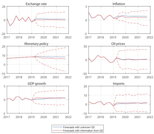
Figure 1 reports a comparison of the unconditional and conditional BVAR projection distribu-tion (the 16th, 50th and 84th quantiles, red dashed lines) for the Mexican macroeconomic scenario. In particular, the top four charts show the dynamics of the exchange rate, inflation, monetary pol-icy rate and oil prices, with known data up to 2019 Q2. The projections suggest that the bilateral exchange rate of the Mexican peso vis-a-vis with the US dollar is expected to depreciate over the forecasting horizon, but in 2019 Q2 there was an unexpected appreciation. Moreover, monetary policy was looser than expected while inflation was lower-than-expected by model, too (consistently with the exchange rate appreciation). Finally, oil prices were in line with model’s expectations.
All charts show corresponding actual data until 2019Q1. For the forecast horizon, 2019:Q2-2021Q4, the solid blue line plots the median forecasts produced by the unconditional model. The red solid line the median forecasts produced by the conditional model while the red-dashed lines make reference to the distribution of the forecasts.
Figure 1: BVAR model projections for Mexico
2017 2018 2019 2020 2021 2022 -20 0 20 Exchange rate 2017 2018 2019 2020 2021 2022 -5 0 5 Inflation 2017 2018 2019 2020 2021 2022 -10 0 10 20 Monetary policy 2017 2018 2019 2020 2021 2022 -50 0 50 Oil prices 2017 2018 2019 2020 2021 2022 -5 0 5 GDP growth 2017 2018 2019 2020 2021 2022 -10 0 10 20 Imports
Forecasts with unknown Q2 Forecasts with information from Q2
BANCO DE ESPAÑA 17 DOCUMENTO OCASIONAL N.º 2001
The bottom two charts show the main target variables. With new information from 2019 Q2, GDP growth is expected to gradually expand over 2019 and inflation is expected to remain below the previous estimation, which increases the purchasing power of agents, together with a more supportive monetary policy.
All charts show corresponding actual data until 2019Q1. For the forecast horizon, 2019:Q2-2021Q4, the solid blue line plots the median forecasts produced by the unconditional model. The red solid line the median forecasts produced by the conditional model while the red-dashed lines make reference to the distribution of the forecasts.
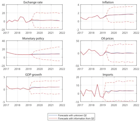
Figure 2 summarizes the same comparison between the unconditional and conditional BVAR projection distributions for the economy of Brazil. As observed, the incoming, up-to-date data for 2019 Q2 do not add relevant information to significantly modify model’s expectations. If anything, inflation rate is expected to be slightly lower, the exchange rate while monetary policy’s predicted path is somewhat looser. In general, the actual data for the exchange rate and monetary policy are quite in line with BVAR model ’s expectations. In this sense, GDP growth projections are slightly lower than the unconditional forecasts, as the model predicts lower demand in the short run, given that inflation has been also lower. This effect is counteracted by higher oil prices, that traditionally has been positively correlated with GDP growth. This relationship might be explained byfiscal factors, by investments in the oil industry or by short-run productivity effects (Kataryniuk and Martínez-Martín, 2019).
Figure 2: BVAR model projections for Brazil
2017 2018 2019 2020 2021 2022 -20 0 20 40 Exchange rate 2017 2018 2019 2020 2021 2022 -2 0 2 4 Inflation 2017 2018 2019 2020 2021 2022 -20 0 20 40 Monetary policy 2017 2018 2019 2020 2021 2022 -50 0 50 Oil prices 2017 2018 2019 2020 2021 2022 -5 0 5 GDP growth 2017 2018 2019 2020 2021 2022 -10 0 10 20 Imports
Forecasts with unknown Q2 Forecasts with information from Q2
Hence, we evaluate the accuracy of conditional BVAR forecasts based on the actual value (i.e. observed ex post) of the future paths of the technical assumptions. Considering the true values of the assumptions, they give rise to forecasts which are not replicable in real time. Such future paths were obviously unknown. However, intuitively, this is the appropriate procedure to evaluate the accuracy of conditional forecasts. In fact, Clark and McCracken (2014) show that the traditional statistics of forecast accuracy retain their statistical properties when evaluating conditional forecasts only if the latter are based on the true value of the "conditions". We compare our BVAR conditional forecasts to the BVAR unconditional forecasts, to gauge if and to what extent our model is able to extract information from the assumptions, and to the forecasts from a univariate benchmark.
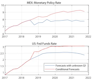
Finally, we generate conditional forecasts depending on the expected monetary policy path in the US, as taken from futures data in February 2019. As can be seen in Figure 3, the monetary policy in Mexico reacts to the monetary policy in the US. In the long run, the BVAR model suggests that monetary policy reaction is higher in Mexico than in the US, pointing to a central bank reaction function that takes into account not only the interest parity condition but also macroprudential concerns stemming from movements in capitalflows.
Figure 3: BVAR model simulations
5.2
Economic response of the Chilean economy to a monetary policy
shock
One of the main uses of economic models is to calibrate the effect that a disturbance identified in the model can have on the rest of the endogenous variables. These disturbances must be structural, in the sense that they are neither determined nor determine the rest of the model’s shocks. As a
20176 2018 2019 2020 2021 2022
7 8 9
10 MEX: Monetary Policy Rate
2017 2018 2019 2020 2021 2022 1 1.5 2 2.5 3
US: Fed Funds Rate
Forecasts with unknown Q1 Conditional Forecasts
BANCO DE ESPAÑA 19 DOCUMENTO OCASIONAL N.º 2001
central bank, a shock which becomes paramaount to understand and deeply analyse is, obviously, a monetary policy shock. Precisely, its effects are those illustrated in this section in the case of the Chilean economy.
Technically, the identification strategy follows the theoretical underpinnings already described in previous sections. Thus, an expansionary monetary policy shock of a structural nature may lead to reductions of interest rates and is correlated with higher GDP growth and inflation. Its economic interpretation is the following: assuming that the interest rate can be approximately determined through a Taylor rule (i.e. the current interest rate depends on the past interest rate, GDP growth, inflation and possibly also on the exchange rate), the pure monetary policy shock would result in a change of the Taylor rule’s residual (i.e. a change in the rate of interest which is not the result of changes in any other explanatory variables such as GDP, inflation and/or exchange rate). This identification strategy allows us to avoid reverse causality issues.
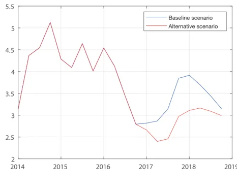
By the beginning of 2017, the Chilean economy faced the possibility that inflation, which was on a downward path, would remain below the central bank target for a protracted period of time, especially if the exchange rate continued to appreciate.12 Given that the Central Bank’s main man-date of price stability, a reduction in interest rates was expected, in line with analysts’ projections in the Economic Expectations Survey (EES) as of March 2017. Such monetary policy loosening would involve a reduction of 50 basis points in the reference 1-year interest rate. The counterfac-tual scenario of interest rates not being reduced by the central bank despite lower inflation would amount to an effective tightening in monetary policy, as the lower inflation would increase the real interest rate.
1 2For further details, see Banco de España Report on the Latin American economy: First half of 2017.
2014 2015 2016 2017 2018 2019 2 2.5 3 3.5 4 4.5 5 5.5 Baseline scenario Alternative scenario
Bank’s objective. Obviously, this increase in inflation would be mainly a consequence of the higher pressure of domestic demand since GDP would grow at rates around 5%, one percentage point more than in the alternative scenario. The greater pressure of domestic demand would be the result of higher spending on consumer goods and investment, which would trigger the substitution, income and wealth effects associated with the reduction in real interest rates.
As shown in Figure 4, in the baseline scenario the monetary policy shock is correlated with a price increase, leading inflation to above the 3% target at the end of 2017. Whereas in the counterfactual scenario, inflation does not return to the target until 2018. The magnitude of the impact of the monetary policy shock on inflation is similar to that reported in other studies of the Chilean economy, such as that of Parrado (2001). In short, monetary policy would be decisive in stabilising inflation in a situation in which price growth deviated from the Central
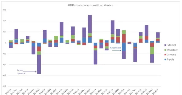
Figure 5: Historical decomposition of GDP growth shocks for Mexico
5.3
Historical decomposition of shocks
This modelling approach is also suitable to determine the structural shocks explaining the recent behaviour of a given economy. This avoids a recurrent issue in conjunctural analysis, namely that of circular reasoning. For instance, whenever a new GDP figure is released along with its expenditure-side disaggregation, an argument often found is that GDP expands due to increased private consumption and this in turn is a consequence of the favorable evolution of the household income. Yet at this aggregate level, the income of households represents most of the GDP. Once one can rely on identifying structural shocks, the “story telling” under this modelling approach becomes quite different. For example, let us assume that the predominant shock in a specific quarter is domestic demand and, in particular, public spending. In such a setting, the narrative would be
BANCO DE ESPAÑA 21 DOCUMENTO OCASIONAL N.º 2001
This kind of exercise has occasionally been presented in reports on some Latin American economies. Specifically, in the second semester of 2016, we made use of this tool in the analy-sis of recent Brazilian behaviour - at that moment the country was suffering a major recession.13
The identification of domestic and external shocks also allow us to construct a historical de-composition of the endogenous variables based on the contributions of the structural shocks. In particular, one can divide the value of any variable for each country in the contribution of the deterministic components and the structural shocks. The appendix provides technical details.
For illustration, we compute the historical decomposition of the model presented in Section 5.1 for Mexico. Figure 5 shows the historical decomposition of GDP growth into identified shocks, starting from 2012 until 2018. We show that the BVAR model is able to identify and quantify two well-known shocks (domestic vs. external) faced by the Mexican economy. As the external shocks are identified with respect to the domestic ones, but not among them, we add up the external shocks as a single contributor. First, the model identifies a significant negative external shock in 2013Q2, which coincides with the episode known as the taper tantrum. The BVAR model´s results also suggest a substraction of quarterly GDP growth by 0.4 percentage points. By the same token, the BVAR model identifies a negative supply shock (the biggest one since the 1990’s) in 2017Q1, related to the liberalization of energy prices, which pushed inflation upwards during the
first quarter of 201714. This shock caused both an increase in inflation and a fall in GDP growth, that amounted to 0.15 pp.
completely different, since that shock would lead firms to face greater demand which will imply
firms hiring more workers. As a result, household income would increase and those households facing credit constraints would then be able to increase private consumption. In addition, higher wages would also have to be paid and inflation would accordingly come under upward pressure, meaning that interest rates would also be affected.
1 3In addition to the historical decomposition of shocks, the macroeconomic effects of afiscal shock (in the form of public expenditure adjustments) were quantified in the second semester of 2016. For further details, see Banco de España Report on the Latin American economy: Second half of 2016.
1 4For further details, please, see Banxico (2017)
6
Concluding remarks
The recent internationalisation of many Spanish banks has made it imperative to monitor the developments in international markets more closely, given the financial stability mandate of the Banco de España. This paper addresses that objective by presenting some of the tools used to analyse macroeconomic developments in those emerging economics which are of material relevance for the Spanishfinancial system. Thus, the paper sets up a macroeconometric modelling approach designed for broad applications to emerging markets, represented here by a small sample of the more relevant countries for Spanish credit institutions: Brazil, Mexico, Turkey, Chile and Peru. We
develop a set of country-specific structural Bayesian VARs and show that our modelling strategy provides useful tools to: (i) analyse the structural shocks that underlie their recent macroeconomic behaviour; (ii) examine the impact of certain decisions of the macroeconomic authorities on a variety of macrofinancial variables (GDP, inflation, etc.) and their interrelationships; and (iii) carry out accurate conditional and unconditional projections two years ahead of the most relevant policy variables. Our results reveal that these tools can be used successfully for an even more in-depth exploration of macroeconomic behaviour in emerging economies. Suggested endeavours include the potential inclusion of other theoretical blocks or the application to a broader sample of countries.
BANCO DE ESPAÑA 23 DOCUMENTO OCASIONAL N.º 2001
References
[1] Arias, J., Rubio-Ramirez, J., and D. Waggoner, (2014). “Inference Based on SVARs Identified with Sign and Zero Restrictions: Theory and Applications”, Board of Governors of the Federal Reserve System International Finance Discussion Papers, No. 1100.
[2] Aguiar, M. and G. Gopinath,(2007). “Emerging Market Business Cycles: The Cycle Is the Trend”, Journal of Political Economy 115, no. 1 (February 2007): 69-102
[3] Banbura, M., D. Giannone and L. Reichlin (2010). “Large Bayesian VARs”,Journal of Applied
Econometrics, No. 25, pp. 71-92.
[4] Banbura, M., D. Giannone and M. Lenza (2015). “Conditional forecasts and scenario analysis with vector autoregressions for large cross-sections”, International Journal of Forecasting, 31(3), pp. 739-756.
[5] Banxico (2017). "Efecto de los Choques Recientes sobre el Proceso Inflacionario en México", Informe Trimestral, Recuadro 2, Abril-Junio 2017.
[6] Canova, F., and M. Ciccarelli (2009). “Estimating Multi-country VAR models",International
Economic Review, 50, 929-961.
[7] Clark, Todd E., and M.W. McCracken (2014). “Evaluating Conditional Forecasts from Vector Autoregressions”, Federal Reserve Bank of St. Louis Working Papers 2014-25.
[8] Del Negro, M., and F. Schorfheide (2013). “DSGE Model-Based Forecasting”, Chapter 2 in Handbook of Economic Forecasting, 2013, vol. 2, pp. 57-140.
[9] De Mol, C., Giannone, D. and L. Reichlin (2008). “Forecasting using a large number of predictors: Is Bayesian shrinkage a valid alternative to principal components?”,Econometric
Reviews, No. 3, pp. 1-100.
[10] Dieppe, A., van Roye, B., and R. Legrand (2016). “The BEAR toolbox”, European Central Bank Working Paper Series, No. 1934.
[11] Doan, T., R. Litterman, and C.A. Sims (1984). “Forecasting and conditional projection using realistic prior distributions”,Journal of Econometrics, 146(2), 318-328.
[12] Gürkaynak, R.S., Kisacikoglu, B., and B. Rossi (2013). “Do DSGE Models Forecast More Accurately Out-of-Sample than VAR Models?”, CEPR Discussion Paper Series, No. 9576. [13] Kataryniuk, I. and J. Martínez-Martín (2019) "TFP growth and commodity prices in emerging
economies" (2019),Emerging Markets Finance and Trade,55(10), pp. 2211-2229
[14] Kilian, L. (2009). “Not All Oil Price Shocks Are Alike: Disentangling Demand and Supply Shocks in the Crude Oil Market”,American Economic Review, Vol. 99 (3), pp. 1053—69.
[15] Litterman, R. (1979). “Techniques of Forecasting Using Vector Autoregressions”, Federal Re-serve of Minneapolis Working Paper, No. 115.
[16] Parrado, E.H. (2001). “Foreign Shocks and Monetary Policy Transmission in Chile”,Journal
Economía Chilena (The Chilean Economy), Central Bank of Chile, vol. 4(3), pp. 29-57.
[17] Rubio-Ramírez, J.F., Waggoner, D.F., and T. Zha (2010). “Structural Vector Autoregressions: Theory of Identification and Algorithms for Inference”, Review of Economic Studies,Oxford University Press, vol. 77(2), pp. 665-696.
[18] Waggoner, D.F. and T. Zha, (1999). “Conditional Forecasts In Dynamic Multivariate Models”,
BANCO DE ESPAÑA 25 DOCUMENTO OCASIONAL N.º 2001
7
Appendix
7.1
Historical decomposition of shocks
A matter of interest in VAR models is to establish the contribution of each structural shock to the historical dynamics of the endogenous variables included in the model. Specifically, for all sample periods, one may wish to decompose the value of each variable into its different components, each component being due to one structural shock of the model. This identifies the historical contribution of each shock to the observed data sample. Thus, any endogenous variable can be separated into two parts: one due to deterministic exogenous variables and initial conditions, and one due to the contribution of unpredictable structural disturbances affecting the dynamics of the model.
For the sake of clarity, let us consider the simplest case where the VAR model has only one lag:
yt=A1yt−1+Cxt+zt (9)
Backward substitution gives:
yt = A1yt−1+Cxt+zt
= A1(A1yt−2+Cxt−1+zt−1) +Cxt+zt
= A1A1yt−2+Cxt+A1Cxt−1+A1zt−1 (10)
By iterating up to the beginning of the sample, in general, for a model withplags, we may rewrite:
yt= p j=1 A(t)j y1−j+ t−1 j=0 Cjxt−j+ t−1 j=0 Bjzt−j (11)
where the matrix series A(t)j , Cj, Bj, are functions of A1, A2, ..., Ap. Note also the matrices B1, B2, ..., Bt−1, provide the response of yt to shocks occurring at periods t, t−1, ..., t−j. By definition, they are result of impulse response function (IRF) matrices:
Bj=ϕj (12)
Therefore, by rearranging we define:
yt= p j=1 A(t)j y1−j+ t−1 j=0 Cjxt−j+ t−1 j=0 ϕjzt−j (13)
and the representation of the IRF in terms of structural shocks:
what may lead us to:
7.2
Conditional forecasts
where thefirst two components are the historical contribution of deterministic variables and the last component is the historical contribution of each structural shock.
To wrap up, bear in mind that this describes the historical decomposition in a traditional, frequentist context. Yet, our Bayesian framework implies uncertainty with respect to the VAR coefficients, so this uncertainty must be integrated into the above framework, and one must compute the posterior distribution of the historical decomposition. As usual, this is done by integrating the historical decomposition framework into the Gibbs sampler, in order to obtain draws from the posterior distribution. Therefore, our empirical SVAR approach is estimated using Bayesian methods to reduce the dimensionality problem with standard Minnesota (or Litterman) priors. In this framework, it is assumed that the VAR residual variance-covariance matrixΣis known. Hence, the only object left to estimate is the vector of parameters. The reported bootstrapping is based on standard errors, percentiles and confidence intervals generated by means of Gibbs sampling procedures after 10,000 repetitions.
yt= p j=1 A(t)j y1−j+ t−1 j=0 Cjxt−j+ t−1 j=0 ϕjσt−j (15)
One may be interested in obtaining what are known as conditional forecasts. These are usually defined as forecasts obtained by constraining the path of certain variables to take specific values. To derive conditional forecasts from our Bayesian SVARs, our approach is based on Waggoner and Zha (1999).
Consider again the VAR model specified in Section 3:
yt=Ct+φ1yt−1+...+φpyt−p+zt, zt∼N(0,Σ) (16)
Assume that one wants to use this model to produce forecasts, and, to make things more concrete, let us consider the simple case of predictingyt+h for a VAR with one lag. By recursive iteration similar to that mentioned above, the forecasts are functions of three terms: (i) terms involving the present value of the endogenous variables yt, terms involving future values of the exogenous variablesxt, and terms involving future values of the reduced form residualszt. As a result, for a forecast of periodT+hfrom a VAR withplags, the following expression is obtained:
yt+h= p j=1 A(h)j yT−j+1+ h j=1 Cj(h)xT+j+ h j=1 Bj(h)zT+j (17)
BANCO DE ESPAÑA 27 DOCUMENTO OCASIONAL N.º 2001
whereA(h)j , Bj(h) , andCj(h)denote the respective matrix coefficients on yT−j+1, zT+j, and xT+j for a forecastyt+h. By defining the corresponding impulse-response function matrices, we rewrite the forecast function in terms of structural shocks:
yt+h= p j=1 A(h)j yT−j+1+ h j=1 Cj(h)xT+j+ h j=1 ϕ(h)h−jτT+j (18)
where thefirst two terms summarise the forecasts in the absence of shocks while the latter represents the dynamic impact of future structural shocks. Therefore, once the system is obtained, it remains to be known how to draw the structural disturbances so that this system of constraint will be satisfied.
In this vein, we rely on Waggoner and Zha (1999), who derive a Gibbs sampling algorithm to construct the posterior predictive distribution of the conditional forecast. In particular, they show that the distribution of the restricted future shocks is normal, and characterised by:
τ ∼N(¯τ,x¯), withτ¯=M(M M )−1m, andx¯=I−M(M M )−1M (19)
It is then possible to use the traditional Gibbs sampler framework to generate draws of the posterior distribution of conditional forecasts, as detailed in the incoming algorithm:
Step 1. Define the total number of iterations of the algorithm, the forecast horizonh, and the
conditions to be imposed: y¯1,y¯2, ...,y¯v.
Step 2. DrawΣ(n),A(n)andb(n)from the corresponding posterior distributions, by recycling
draws from the Gibbs sampler at iterationn.
Step 3. Compute the unconditional forecasts: y(T+1), ..., y(T+h).
Step 4. Compute the impulse response function matrices τj and ¯τjfrom the constrained
variables.
Step 5. Build M andm, as defined above, and draw the constrained shocks.
Step 6. Calculate the conditional forecast using [20] according to the unconditional forecasts
BANCO DE ESPAÑA PUBLICATIONS
OCCASIONAL PAPERS
1501 MAR DELGADO TÉLLEZ, PABLO HERNÁNDEZ DE COS, SAMUEL HURTADO and JAVIER J. PÉREZ: Extraordinary mechanisms for payment of General Government suppliers in Spain. (There is a Spanish version of this edition with the same number).
1502 JOSÉ MANUEL MONTERO y ANA REGIL: La tasa de actividad en España: resistencia cíclica, determinantes y perspectivas futuras.
1503 MARIO IZQUIERDO and JUAN FRANCISCO JIMENO: Employment, wage and price reactions to the crisis in Spain: Firm-level evidence from the WDN survey.
1504 MARÍA DE LOS LLANOS MATEA: La demanda potencial de vivienda principal.
1601 JESÚS SAURINA and FRANCISCO JAVIER MENCÍA: Macroprudential policy: objectives, instruments and indicators. (There is a Spanish version of this edition with the same number).
1602 LUIS MOLINA, ESTHER LÓPEZ y ENRIQUE ALBEROLA: El posicionamiento exterior de la economía española. 1603 PILAR CUADRADO and ENRIQUE MORAL-BENITO: Potential growth of the Spanish economy. (There is a Spanish
version of this edition with the same number).
1604 HENRIQUE S. BASSO and JAMES COSTAIN: Macroprudential theory: advances and challenges.
1605 PABLO HERNÁNDEZ DE COS, AITOR LACUESTA and ENRIQUE MORAL-BENITO: An exploration of real-time revisions of output gap estimates across European countries.
1606 PABLO HERNÁNDEZ DE COS, SAMUEL HURTADO, FRANCISCO MARTÍ and JAVIER J. PÉREZ: Public fi nances and infl ation: the case of Spain.
1607 JAVIER J. PÉREZ, MARIE AOURIRI, MARÍA M. CAMPOS, DMITRIJ CELOV, DOMENICO DEPALO, EVANGELIA PAPAPETROU, JURGA PESLIAKAITĖ, ROBERTO RAMOS and MARTA RODRÍGUEZ-VIVES: The fi scal and macroeconomic effects of government wages and employment reform.
1608 JUAN CARLOS BERGANZA, PEDRO DEL RÍO and FRUCTUOSO BORRALLO: Determinants and implications of low global infl ation rates.
1701 PABLO HERNÁNDEZ DE COS, JUAN FRANCISCO JIMENO and ROBERTO RAMOS: The Spanish public pension system: current situation, challenges and reform alternatives. (There is a Spanish version of this edition with the same number). 1702 EDUARDO BANDRÉS, MARÍA DOLORES GADEA-RIVAS and ANA GÓMEZ-LOSCOS: Regional business cycles
across Europe.
1703 LUIS J. ÁLVAREZ and ISABEL SÁNCHEZ: A suite of infl ation forecasting models.
1704 MARIO IZQUIERDO, JUAN FRANCISCO JIMENO, THEODORA KOSMA, ANA LAMO, STEPHEN MILLARD, TAIRI RÕÕM and ELIANA VIVIANO: Labour market adjustment in Europe during the crisis: microeconomic evidence from the Wage Dynamics Network survey.
1705 ÁNGEL LUIS GÓMEZ and M.ª DEL CARMEN SÁNCHEZ: Indicadores para el seguimiento y previsión de la inversión en construcción.
1706 DANILO LEIVA-LEON: Monitoring the Spanish Economy through the Lenses of Structural Bayesian VARs. 1707 OLYMPIA BOVER, JOSÉ MARÍA CASADO, ESTEBAN GARCÍA-MIRALLES, JOSÉ MARÍA LABEAGA and
ROBERTO RAMOS: Microsimulation tools for the evaluation of fi scal policy reforms at the Banco de España. 1708 VICENTE SALAS, LUCIO SAN JUAN and JAVIER VALLÉS: The fi nancial and real performance of non-fi nancial
corporations in the euro area: 1999-2015.
1709 ANA ARENCIBIA PAREJA, SAMUEL HURTADO, MERCEDES DE LUIS LÓPEZ and EVA ORTEGA: New version of the Quarterly Model of Banco de España (MTBE).
1801 ANA ARENCIBIA PAREJA, ANA GÓMEZ LOSCOS, MERCEDES DE LUIS LÓPEZ and GABRIEL PÉREZ QUIRÓS: A short-term forecasting model for the Spanish economy: GDP and its demand components.
1802 MIGUEL ALMUNIA, DAVID LÓPEZ-RODRÍGUEZ and ENRIQUE MORAL-BENITO: Evaluating the macro-representativeness of a fi rm-level database: an application for the Spanish economy.
1803 PABLO HERNÁNDEZ DE COS, DAVID LÓPEZ RODRÍGUEZ and JAVIER J. PÉREZ: The challenges of public deleveraging. (There is a Spanish version of this edition with the same number).
1804 OLYMPIA BOVER, LAURA CRESPO, CARLOS GENTO and ISMAEL MORENO: The Spanish Survey of Household Finances (EFF): description and methods of the 2014 wave.
1805 ENRIQUE MORAL-BENITO: The microeconomic origins of the Spanish boom.
1807 MAR DELGADO-TÉLLEZ and JAVIER J. PÉREZ: Institutional and economic determinants of regional public debt in Spain. 1808 CHENXU FU and ENRIQUE MORAL-BENITO: The evolution of Spanish total factor productivity since the Global Financial Crisis.
1809 CONCHA ARTOLA, ALEJANDRO FIORITO, MARÍA GIL, JAVIER J. PÉREZ, ALBERTO URTASUN and DIEGO VILA: Monitoring the Spanish economy from a regional perspective: main elements of analysis.
1810 DAVID LÓPEZ-RODRÍGUEZ and CRISTINA GARCÍA CIRIA: Estructura impositiva de España en el contexto de la Unión Europea.
1811 JORGE MARTÍNEZ: Previsión de la carga de intereses de las Administraciones Públicas.
1901 CARLOS CONESA: Bitcoin: a solution for payment systems or a solution in search of a problem? (There is a Spanish version of this edition with the same number).
1902 AITOR LACUESTA, MARIO IZQUIERDO and SERGIO PUENTE: An analysis of the impact of the rise in the national minimum wage in 2017 on the probability of job loss. (There is a Spanish version of this edition with the same number). 1903 EDUARDO GUTIÉRREZ CHACÓN and CÉSAR MARTÍN MACHUCA: Exporting Spanish fi rms. Stylized facts and trends. 1904 MARÍA GIL, DANILO LEIVA-LEON, JAVIER J. PÉREZ and ALBERTO URTASUN: An application of dynamic factor
models to nowcast regional economic activity in Spain.
1905 JUAN LUIS VEGA (COORD.): Brexit: current situation and outlook.
1906 JORGE E. GALÁN: Measuring credit-to-GDP gaps. The Hodrick-Prescott fi lter revisited.
1907 VÍCTOR GONZÁLEZ-DÍEZ and ENRIQUE MORAL-BENITO: The process of structural change in the Spanish economy from a historical standpoint. (There is a Spanish version of this edition with the same number).
1908 PANA ALVES, DANIEL DEJUÁN and LAURENT MAURIN: Can survey-based information help assess investment gaps in the EU?
1909 OLYMPIA BOVER, LAURA HOSPIDO and ERNESTO VILLANUEVA: The Survey of Financial Competences (ECF): description and methods of the 2016 wave.
1910 LUIS JULIÁN ÁLVAREZ: El índice de precios de consumo: usos y posibles vías de mejora.
1911 ANTOINE BERTHOU, ÁNGEL ESTRADA, SOPHIE HAINCOURT, ALEXANDER KADOW, MORITZ A. ROTH and MARIE-ELISABETH DE LA SERVE: Assessing the macroeconomic impact of Brexit through trade and migration channels.
1912 RODOLFO CAMPOS and JACOPO TIMINI: An estimation of the effects of Brexit on trade and migration. 1913 ANA DE ALMEIDA, TERESA SASTRE, DUNCAN VAN LIMBERGEN and MARCO HOEBERICHTS: A tentative
exploration of the effects of Brexit on foreign direct investment vis-à-vis the United Kingdom.
1914 MARÍA DOLORES GADEA-RIVAS, ANA GÓMEZ-LOSCOS and EDUARDO BANDRÉS: Ciclos económicos y clusters
regionales en Europa.
1915 MARIO ALLOZA and PABLO BURRIEL: La mejora de la situación de las fi nanzas públicas de las Corporaciones Locales en la última década.
1916 ANDRÉS ALONSO and JOSÉ MANUEL MARQUÉS: Financial innovation for a sustainable economy. (There is a Spanish version of this edition with the same number).
2001 ÁNGEL ESTRADA, LUIS GUIROLA, IVÁN KATARYNIUK and JAIME MARTÍNEZ-MARTÍN: The use of BVARs in the analysis of emerging economies.
Unidad de Servicios Auxiliares Alcalá, 48 - 28014 Madrid E-mail: [email protected]