Experimental investigation of nonequilibrium and separation scaling in double-wedge and double-cone geometries

(1)

c

(2)

EXPERIMENTAL INVESTIGATION OF NONEQUILIBRIUM AND SEPARATION SCALING IN DOUBLE-WEDGE AND DOUBLE-CONE

GEOMETRIES

BY

ANDREW MARSHALL KNISELY

DISSERTATION

Submitted in partial fulfillment of the requirements for the degree of Doctor of Philosophy in Aerospace Engineering

in the Graduate College of the

University of Illinois at Urbana-Champaign, 2016

Urbana, Illinois Doctoral Committee:

Associate Professor Joanna Austin, Director Professor J. Craig Dutton, Chair

Assistant Professor Marco Panesi Associate Professor Tonghun Lee

(3)

ABSTRACT

Experiments were performed in the Hypervelocity Expansion Tube (HET) and the T5 hypervelocity shock tunnel to investigate geometric and gas composition effects on a double-wedge and double-cone geometry. The high-speed flow over the models results in a complex shock boundary-layer interaction which is known to be sensitive to thermal and chemical nonequilibrium. High-speed shadowgraph and surface heat flux measurements are obtained for both geometries. Surface heat flux measurements of the laminar boundary layer for the double-wedge show good agreement between both facilities with proper nondimensionalization. High-speed shadowgraph imaging is used to study the flowfield startup processes. The shock interactions and separation location exhibit no transient processes once the nozzle reservoir reaches a steady stagnation pressure level in T5. Two of the primary shock-shock interaction types are identified for the double-cone. Augmented heat flux is observed for the Edney Type V interactions with the highest peak heating observed with the nitrogen test gas. However, transient heat flux measurements during the nozzle startup indicate that the peak heat flux is not captured by the thermocouples for the air case due to the highly local nature of heating in this shock configuration.

The boundary-layer separation scaling based on triple-deck theory for a wedge is applied to the cone geometry. The pressure correlation for the double-cone is found to be in agreement with historical results. No significant response of the separation length to the gas composition, apart from changes in the freestream condition, are observed for the current experiments. In purely laminar interactions no dependence of the scaled separation on Reynolds number is observed. Reattachment heat flux indicates transitional behavior of the separated boundary layer for the high

(4)

Reynolds number conditions. A consistent decrease in scaled separation length is found for transitional interactions.

(5)

ACKNOWLEDGMENTS

Thanks first goes to my advisor, Professor Joanna Austin. From my initial summer REU position through today you have given me many great opportunities and guid-ance through my graduate career. Next, I’d like to thank my committee members Professors Craig Dutten, Marco Panesi, and Tonghun Lee for taking the time to pro-vide guidance, suggestions, and critiques of this work. I would also like to thank Professor Hans Hornung at Caltech for sharing his incredible wealth of knowledge about all things related to high-speed gas dynamics.

Thanks goes to my friends and classmates at Illinois. Special thanks goes to Bill Flaherty, Ryan Fontaine, and Andy Swantek who have been great friends, colleagues, and mentors. From teaching me to run the HET to helping with a new diagnostic, I would not be the experimentalist I am today without their help. Also thanks to Todd Reedy, Tommy Herges, and Manu Sharma for help in and around different facilities, learning about high-speed gas dynamics, and debugging MATLAB scripts. Galina Shpuntova and Matt Leibowitz, not only have I had the pleasure of working with you but you have been a strong source of support as we made the trek out West. To everyone else from Illinois that I have had the pleasure of knowing, you have all been great friends both in and out of work.

I want to thank all of the wonderful people I have meet at Caltech with special mention of three individuals. Bryan Schmidt, it was great working with you and getting to know your family and I am very grateful for your assistance in getting T5 operational again. Thanks also to Joe Jewell who spent many hours talking with me as I worked to recommission T5 and understand the underlying physics of the facility. Lastly, the success of this work would not have been possible without the tireless help

(6)

of Bahram Valiferdowsi in keeping T5 up and running.

I want to thank my parents for their unwavering support throughout my life. Mom and Dad, you have challenged me to always do my best both in and out of school and never give up no matter what issue may arise. To my brothers, Ben and Joey, I am always so grateful when we find time to get together and I wish you both the best of luck as you both embark on your own new adventures.

Lastly, to Christina, without your love and support I would never have had the courage to finish.

(7)

LIST OF TABLES

2.1 Nominal HET run conditions. . . 17

2.2 Nominal T5 run conditions. Conditions on a shot-by-shot basis are included in Appendix A. . . 18

2.3 Nominal T5 run conditions mass fractions. Values designated as ‘–’ have mass fractions less than 1×10−9. . . 18

2.4 Normalized location of double-wedge thermocouples . . . 20

2.5 Normalized location of 25-55 double-cone thermocouples . . . 21

2.6 Normalized locations of coaxial thermocouples on the 25-48 double-cone model. . . 22

3.1 Comparison of property values for regions 7 and 8 for the Type V shock interaction for Shot 2860. . . 51

3.2 Bow shock standoff distance and post-shock mean density ratio. . . . 51

4.1 Mean peak heat flux levels for T5 25-48 double-cone. . . 65

4.2 Measured peak mean heat flux level for T5 25-55 double-cone. . . 71

5.1 Values of axisymmetric asymptotic triple-deck parameters to deter-mine flow regime. . . 93

A.1 Measured shot conditions and calculated nozzle reservoir conditions. . 109

A.2 Freestream shot conditions . . . 110

A.3 Region 1 calculated shot conditions . . . 111

A.4 Region 1 calculated mass fractions . . . 112

A.6 Region 2 calculated mass fractions . . . 114

(9)

LIST OF FIGURES

1.1 Diagram of the flow structure for the double-cone. . . 2

2.1 Image of double-wedge model . . . 8

2.2 T5 25-55 double-cone installed in the test section. . . 9

2.3 Diagrams of the 25-48 and 25-55 T5 double-cone models. Dimen-sions are given in mm. . . 10

2.4 Image of HET . . . 11

2.5 Labeled diagram of T5. . . 13

2.6 Shock Timing Pressure Transducers, Shot 2876 . . . 14

2.7 Nozzle Reservoir Transducers, Shot 2876 . . . 15

2.8 Diagram of HET schlieren setup. . . 25

2.9 Image of the Shimadzu HPV-X2 camera used for the high-speed shadowgraph images obtained in T5. . . 26

2.10 Sony SLDV1332V laser diode and PicoLAS LDP-V 03-100 UF3 driver module . . . 27

2.11 Schematic of T5 shadowgraph setup. . . 27

3.1 T5 double-wedge startup process, Shot 2851 . . . 31

3.2 Labeled image of established flowfield for 25-55 double-cone. . . 33

3.3 T5 25-55 H8-Re2 nitrogen double-cone startup process, Shot 2856 . . 34

3.4 T5 25-55 double-cone H8-Re2 air startup process, Shot 2858 . . . 35

3.5 T5 25-55 double-cone H8-Re2 CO2 startup process, Shot 2875 . . . . 37

3.6 T5 25-55 double-cone H8-Re6 nitrogen startup process, Shot 2862 . . 38

3.7 T5 25-55 double-cone H8-Re6 air startup process, Shot 2861 . . . 40

3.8 Labeled image of established flowfield for 25-48 double-cone. . . 41

3.9 T5 25-48 double-cone H8-Re2 Air startup process, Shot 2878 . . . 42

3.10 Schematic of type VI interaction with labeled regions for shock polar diagrams. . . 45

3.11 Shot 2879, H8-Re2 Air 25-48 double-cone . . . 46

3.12 Shot 2881, H8-Re2 CO2 25-48 double-cone . . . 46

3.13 Shot 2877, H8-Re2 N2 25-48 double-cone . . . 47

3.14 Shot 2882, H8-Re6 Air 25-48 double-cone . . . 48

(10)

4.1 Image of cone grid used for viscous single cone simulations used to

extract the laminar boundary layer heat flux. . . 58

4.2 Pressure and temperature fields from DPLR of shot 2853. . . 59

4.3 Mean heat flux and labeled shadowgraph for the H8-Re2 air condi-tion with the double-wedge in T5. . . 60

4.4 Normalized mean heat flux for double-wedge in T5 and the HET. . . 61

4.5 Mean heat flux and shadowgraph for the H8-Re2 N2 run condition with the double-wedge in T5. . . 62

4.6 Heat flux and labeled shadowgraph for the H8-Re2 nitrogen run condition with the 25-48 double-cone. Shadowgraph from shot 2877. . 66

4.7 Heat flux and labeled shadowgraph for the H8-Re2 air run condition with the 25-48 double-cone. Shadowgraph from shot 2879. . . 68

4.8 Heat flux and labeled shadowgraph for the H8-Re2 carbon dioxide run condition with the 25-48 double-cone. Shadowgraph from shot 2881. 69 4.9 Heat flux and labeled shadowgraph for the H8-Re6 air run condition with the 25-48 double-cone. Shadowgraph from shot 2882. . . 70

4.14 Heat flux and labeled shadowgraph for the H8-Re2 carbon dioxide run condition with the 25-55 double-cone. Shadowgraph from shot 2875. 77 4.15 Mean heat flux comparison of gas composition for the H8-Re2 con-dition with the 25-55 double-cone. . . 78

4.16 Mean heat flux comparison of air and nitrogen for the H8-Re6 con-dition with the 25-55 double-cone. . . 78

4.17 Transient heat flux trace and shadowgraph images, Shot 2858, Ther-mocouple A-11 . . . 80

4.18 Normalized mean heat flux for double-cone in N2 for T5 . . . 81

4.19 Normalized mean heat flux for double-cone in air for T5 . . . 82

4.20 Normalized mean heat flux for double-cone in N2 for T5 . . . 83

4.21 Normalized mean heat flux for double-cone in air for T5 . . . 83

5.1 Labeled diagram of the double-wedge flow field. This diagram shows only the flow structures relevant to the separation scaling theory. . . 87

5.2 Diagram of control volume proposed by Sychev [19] and Roshko [18]. 87 5.3 Diagram of laminar boundary layer transitioning to triple-deck struc-ture. The names of the decks are shown along with height written in terms of the scaling parameter. . . 88

(11)

5.4 Measured separation scaling parameters labeled on shadowgraph

image of double-wedge flow . . . 95

5.5 Separation length for double-wedge in T5. . . 96

5.6 Separation length for double-wedge in T5. . . 97

5.7 Labeled measured variables used for separation scaling for the double-cone flowfield. . . 98

5.8 Scaled separation length versus normalized pressure rise for the double-cone in T5 and the HET . . . 100

5.9 Scaled separation length versus Reynolds number for the double-cone in T5 and the HET . . . 101

5.10 Scaled separation length plotted against separated shear layer Reynolds number. . . 103

5.11 Shadowgraph image of out-of-plane image artifact . . . 104

B.1 Mean heat flux results for Shot 2853, H8-Re2 N2 . . . 118

B.5 Mean heat flux results for Shot 2857, H8-Re2 Air . . . 120

B.13 Mean heat flux results for Shot 2874, H8-Re2 CO2 . . . 124

C.1 T5 25-55 double-cone . . . 129

C.2 T5 25-55 double-cone thermocouple hole locations . . . 130

C.3 T5 25-55 double-cone tip modification . . . 131

C.4 T5 double-cone tip . . . 132

(12)

CHAPTER 1

INTRODUCTION

1.1

Background

Hypersonic shock boundary-layer interactions involve complex interactions between various viscous and inviscid processes [1, 2]. These interactions are of both academic and practical interest as these interaction are very common on high-speed air breath-ing and re-entry type vehicles, such as the Boebreath-ing X-51 [3]. Shock boundary-layer interactions introduce difficulties to the design and control of these vehicles due to potential flow unsteadiness and high levels of peak heating. Thus it is imperative to be able to make accurate predictions of both pressure and heat flux loads on the vehicle surfaces.

The model problem presented is high-stagnation-enthalpy hypervelocity flow over a double-wedge and double-cone geometry. A diagram of the flowfield is shown in Fig-ure 1.1. An incoming laminar boundary layer interacts with a shock system formed by the interaction of an oblique and bow shock. The flow separates forming a com-plex shock dominated turbulent flow with impingement on the surface. Additional reactions are occurring due to the high temperatures behind the bow shock and in the shock impingement region. This shock-boundary-layer interaction is known to be very sensitive to the thermochemical state of the gas [4–6]. This strong coupling between thermochemistry and shock boundary layer interaction makes the double-wedge and double-cone sensitive test cases for model development [3,7]. Experiments and numerical simulations have been completed on double-cone and double-wedge flows with the same freestream conditions. Good agreement between experiments and simulations have been found at low enthalpy conditions while poor agreement is

(13)

seen at high enthalpy conditions [5–7]. A more detailed overview of these studies is made in the following paragraphs.

Oblique Shock

Separation

Shock

Bow Shock

Shear

Layer

Reattachment

Shock

Separation Zone

Ψ

*

1

2

3

Boundary Layer

M

_∞

Figure 1.1: Diagram of the flow structure for the double-cone.

Thermochemical nonequilibrium has been identified as one of the key components of the double-wedge and double-cone flow field. Thermochemical nonequilibrium is the umbrella term used to describe chemical and vibrational nonequilibrium charac-teristics of hypersonic flows. A simple description of the terms is given here. These conditions can be explained by considering the relaxation region behind a normal shock in front of a body in high-speed flow. The normal shock causes an instan-taneous increase in temperature, pressure and density. If the shock is sufficiently strong, the post-shock gas will undergo chemical reactions leading to a drop in tem-perature and an increase in pressure and density. This region of chemical activity is known as the relaxation region. If the distance between the shock and the body is sufficiently larger than the relaxation distance, the gas can be considered to be in equilibrium. The flow is considered to be frozen if the opposite scenario exists, that is the relaxation length is much longer than distance between the shock and the model. In this case the gas has no time for reactions to occur before interacting with

(14)

another body. Chemical nonequilibrium exists in the region bounded by frozen and equilibrium conditions. This third case exists when these two length scales are on the same order and now the rate of chemical reactions is required in order to make accurate predictions to the chemical state of the gas. Additionally, the vibrational state of the gas changes at a finite rate due to the transfer of energy by molecular collisions. When the gas temperature jumps dues to the shock, collisions between the molecules redistribute the energy into the vibrational modes. If the gas is given a sufficient length of time, the vibrational energy reaches its equilibrium state. Vi-brational nonequilibrium exists in the time during which the viVi-brational energy is changing. Chemical and vibrational nonequilibrium may be present simultaneously. Additionally, coupling between the two exists, e.g., dissociation rates may be higher for vibrationally exited gases.

Computational and experimental work using the double-cone and double-wedge geometry have focused on improving thermochemical models such that accurate sim-ulations can be made. Previous double-wedge work has shown discrepancies between the size of the separation and an under-prediction of pressure levels between experi-mental and simulations [8]. Nitrogen dissociation rates could not solely account for the discrepancies and other issues such as freestream modeling, spanwise effects, or unsteadiness were offered as possible explanations. Double-cone studies were com-pleted to remove issues related to the double-wedge geometry [9]. These two studies showed that equilibrium nitrogen dissociation rates for realistic geometries in hyper-sonic flows were not modeled well. Additionally, nonequilibrium nitrogen dissociation rates were also not well modeled due to poor vibration-dissociation coupling mod-els [9]. In addition to the vibrational-dissociation modmod-els, freestream vibrational freezing must be considered to accurately compare simulations with experimental results [5]. The addition of oxygen to the flow field introduces many chemical reac-tions and species such as NO. Non-Boltzmann distribureac-tions of NO have been seen in reacting regions through the second Zel’dovich mechanism [10]. Additionally, poor prediction of oxygen recombination has been theorized as another possible reason for

(15)

Shock interaction types between an oblique shock and cylinder bow shock were first extensively defined by Edney [12]. In this paper Edney studied augmented heat flux and pressure levels on a cylinder with an oblique shock impingement. The shock interactions were classified into six main groups, Types I-VI. Sanderson [13] studied nonequilibrium effects due to thermochemistry for this flowfield. Olejniczak et al. [14] performed inviscid simulations of a double-wedge and was able to observe four of the shock interaction types. However, there are differences in the interaction structures observed by Olejniczak compared to the interactions as defined by Edney due to con-straints placed on the flow by the model geometry. Experimental measurements at low Reynolds number of the double-cone flowfield in a hypersonic blowdown facility showed good agreement with laminar simulations for the separation size and inter-action type [15]. Higher enthalpy double-wedge and double-cone experiments have also made observations of the different shock interaction types [16, 17]. Jangadeesh et al. [16] observed unsteady flow for high deflection angles with a double-cone. A type V interaction was observed for a 25◦–50◦ double-cone.

A scaling law for the separated boundary layer of a double-wedge has been devel-oped by Davis and Sturtevant [4]. This scaling law is built by applying triple-deck theory to a base-flow model. The base flow model, introduced by Roshko [18], de-scribes the application of a theory of pressure rise through a shear layer by Sychev [19]. Triple-deck theory has been studied extensively by Stewartson and Williams and describes the region near a boundary layer that separates due to a disturbance in the flow field [20, 21]. Triple-deck theory has also been studied for other geometries such as two-dimensional compression corners and axisymmetric geometries. Rizzetta, Burggraf and Jenson studied separation of boundary layers at two-dimensional com-pression corners [22]. They note that corner angle, α∗, must be O(Re−1/4) for the simplified triple deck formulation to hold. When the angle is smaller, separation does not occur and when the angle is larger a more complicated structure forms, which has been previously analyzed by Burggraf [23]. Triple-deck theory applied to axisymmet-ric bodies has been studied with applications to cylinders and flared cones [24–28]. Flared cylinders have been the focus of several of these studies [24,25,28]. A brief

(16)

con-sideration of geometries with inclined forebodies such as the double-cone was made by Huang and Inger [25].

One important consideration to make is whether three-dimensional effects have an impact on a nominally two-dimensional flow field, such as a planar compression corner. Experimental and theoretical studies of hypersonic compression corners were completed by Holden and Moselle [29]. Two-dimensional flow was determined by ob-serving successively wider models until no change in measurements at the centerline was observed. Rudy et al. [30] completed two-dimensional simulations of the Holden and Moselle experiments. They find that two-dimensional computations do not match the experimental results for highly-separated flow fields. Three-dimensional simula-tions completed match both the separation length and the time to steady flow indicat-ing that spanwise effects may be important in a nominally two-dimensional flow field. However, simulations completed by Lee and Lewis [31] show that two-dimensional simulations are able to replicate the experimental and three-dimensional simulation results. Hypersonic high enthalpy shock boundary layer interactions in compression corners have been studied by Mallinson, Gai and Mudford [32, 33]. They also note that two-dimensional flow can be achieved even for highly-separated flows.

1.2

Overview of Current Work

The previous work discussed above has shown that thermochemistry and geometry can significantly affect the hypersonic shock-bondary layer interaction over a double-wedge and double-cone geometry. At the conditions being studied the thermochemical effects of oxygen chemistry can be isolated by switching between air and nitrogen test gas. The current work evaluates the effects of gas composition on both viscous and inviscid flow features. Special consideration is taken to study effects on flow estab-lishment and steadiness. The second main goal of the project will be to determine the role of an axisymmetric body-geometry on this scaling parameter. The separa-tion scaling parameter developed previously for the double-wedge geometry is built

(17)

scaling is the incorporation of triple-deck asymptotic theory. This framework will be examined for a double-cone using experimental measurements in two facilities.

Chapter 2 describes the experimental methods used in this study. This includes the model design, facility descriptions, diagnostic techniques used, and the details of flow conditions. Chapter 3 includes analysis of the flow startup and of shock structures through high-speed shadowgraph. Chapter 4 summarizes the heat flux results for the double-wedge and double-cone. Chapter 5 includes an analysis of the separation scaling. Lastly, Chapter 6 contains the conclusions and summary of the work completed.

(18)

CHAPTER 2

EXPERIMENTAL SETUP

The model geometries studied and the experimental facilities used are described in this chapter. Details’ on both facilities capabilities and operation are provided. The freestream conditions are reported with an explanation of the methods used for their calculation. The measurement techniques used to collect data are described with focus on the setup and equipment used.

2.1

Model Geometries

Two model geometries, a double-wedge and double-cone are used. These geometries were initially chosen due to their historical significance allowing for comparisons to be made with previous experimental and numerical studies.

2.1.1

Double-Wedge

The double-wedge model is a fore wedge angle of 30◦ and aft wedge angle of 55◦. The primary model has a front face length of 50.8 mm, aft face length of 25.4 mm, and span length of 101.6 mm. An image of the double-wedge model is shown in Figure 2.1. The double-wedge is machined from A2 tool steel and is constructed from two parts to allow for easy internal access for thermocouple installation. The double-wedge model was used for tests in the HET and T5. Additional details on the design and construction of the double-wedge model may be found in Swantek [17].

(19)

Figure 2.1: Image of double-wedge model. The model is shown before the installation of additional thermocouples for the T5 tests. Image courtesy of Swantek [17].

2.1.2

Double-Cone

The second model geometry used is the double-cone. Two double-cone geometries are used in this study with the primary cone geometry having a front half-angle of 25◦ and aft half-angle of 55◦. The double-cone geometry was chosen to eliminate finite span effects inherent to the double-wedge model.

The 25-55 double-cone model is based on the design of Nompelis et al. [5] Two physical models of this double-cone are used for this work. The first model, con-structed by Swantek [34], was used in the HET. This model has a first base diameter of 25 mm and a second base diameter of 63.5 mm. The model is made from A2 tool steel and assembled from two parts to avoid any curvature at the hinge location. No thermocouples are instrumented into the model due to space constraints.

The second 25-55 double-cone model was machined for use in T5. This double-cone model is an enlarged scale model of the HET version. The T5 model has a first base diameter of 48.2 mm and a second base diameter of 122.3 mm, shown in Figure 2.2. The size of the model was increased from the HET double-cone so that thermocouples can be installed into the model. A total of 64 thermocouples are installed to allow for heat flux measurements. The tip is made from molybdenum and is designed to be replaceable in case of damage or wear due to the high heat flux loads present at

(20)

the tip.

Figure 2.2: T5 25-55 double-cone installed in the test section.

The second double-cone geometry used in T5 has a fore cone half-angle of 25◦ and aft cone angle of 48◦. The first and second base diameters of this model are the same as the other T5 double-cone model. By maintaining the same fore cone geometry, the effects due to reduced flap angle on the triple point interaction and reattachment shock can be isolated. Additionally, thermocouples are only installed onto the aft cone since the fore cone geometry has remained unchanged. Both T5 double-cone models are installed inline with the nozzle axis and with a measured pitch of less than±0.1◦. Through this work both double-cone models will be referenced based on the fore and aft cone half-angles, i.e. the 25-55 double-cone or 25-48 double cone.

2.2

Facility

Experiments are completed in two facilities: the Hypervelocity Expansion Tube (HET) and the T5 free-piston driven reflected-shock tunnel.

2.2.1

HET

(21)

(a) 25-48 Double-Cone (b) 25-55 Double-Cone

Figure 2.3: Diagrams of the 25-48 and 25-55 T5 double-cone models. Dimensions are given in mm.

of obtaining a range of freestream conditions with Mach numbers from 3 to 7.5 and stagnation enthalpies of 2 to 9 MJ/kg. The HET consists of three sections: a driver, driven, and expansion section. The total length of the HET is 9.14 m with an inner diameter of 152 mm and is constructed of 304/304L stainless steel. Two final sections, the test section and dump tank, are located downstream of the expansion section. The models are installed into the test section which connects to the expansion section through a sliding seal. An image of the facility from the test section is seen in Figure 2.4.

The driver and driven sections are separated by an aluminum diaphragm. This diaphragm is made from 5052 aluminum and is varied in thickness to change the driver gas burst pressure. The primary diaphragm ruptures naturally as the driver section is filled with gas, typically helium, which presses the diaphragm against a set of knife blades. Using the knife blades increases the shot-to-shot repeatability and prevents metal shards from detaching and damaging the facility and models downstream. The rupture of the primary diaphragm causes a strong shock wave to travel down the driven section, compressing and accelerating the test gas. The expansion section is initially separated from the driven section by a thin mylar diaphragm. When ruptured

(22)

Figure 2.4: Image of HET looking upstream from test section.

by the incident shock, a transmitted shock and unsteady expansion fan form. The unsteady expansion fan further accelerates the shocked test gas to the test condition. The test gas then exits the tube into a test section which has optical access from three sides. Additional details of the facility design, construction, operation and characterization are found in Dufrene, Sharma, and Austin [35].

The HET data acquisition (DAQ) system is comprised of two PXI-6133 data ac-quisition cards housed in a PXI-1031 chassis. The PXI-6133 card is capable of 8 simultaneous analog inputs with acquisition rates up to 2.5 MHz at 14-bit resolution. Data is recorded at 1 MHz for 30 ms with a pretrigger time of 12 ms. Each DAQ card is connected to a BNC-2110 block which is used to connect with the pressure trans-ducers and heat flux gauges. The DAQ system is controlled through an NI Labview VI running on a Microsoft Windows system. The driver pressure is recorded using a Setra Model 206 pressure sensor. A total of four PCB 113A26 piezoelectric pressure transducers are installed along the tube to measure wave speeds and as a secondary method for triggering the DAQ system. Three MKS capacitance manometers are used to measure the vacuum levels in the driven and expansion section. These three gauges are only used before the experiment is run and are not recorded due to the possibility of damage from the primary shock wave. An additional PCB 113A26

(23)

pres-sure transducer is used in the test section as a pitot probe and is used as the primary trigger for the DAQ system.

2.2.2

T5

The T5 free-piston reflected shock tunnel is another impulse facility that is able to produce a hypervelocity freestream. The two facilities are able to produce overlap-ping freesteam conditions while utilizing different gas acceleration methods. The T5 facility utilizes a piston to adiabatically compress a helium/argon mixture to high pressure which acts as the driver to a reflected shock tunnel [36]. The facility con-sists of five main sections: the compression tube, secondary reservoir, shock tube, test section, and dump tank. A diagram of the facility is shown in Figure 2.5. A stainless steel diaphragm initially separates the compression tube and shock tube. This diaphragm is pre-scored to a prescribed depth based on previous experiments to achieve a repeatable burst pressure. The scoring also ensures that the diaphragm breaks in a predictable manner and that no metal petals become detached. A nozzle is located at the other end of the shock tube and slides into the test section. A thin mylar diaphram located within the nozzle throat region is used to separate the shock tube from the test section and dump tank.

To run an experiment, a 120 kg piston in loaded into the end of the compression tube and the entire facility is initially evacuated using a combination of vacuum pumps. The shock tube is then filled with the test gas, typically air, nitrogen, carbon-dioxide or some mixture thereof. The compression tube is filled with a helium/argon gas mixture and the secondary reservoir is filled with compressed air. Once the pressures are set, a fast acting valve, located between the compression tube and secondary reservoir, is opened which allows the compressed gas to empty into the piston space located behind the piston causing it to accelerate down the compression tube. The piston adiabatically compresses the helium/argon mixture in front of it and once the gas reaches a sufficiently high pressure the primary diaphragm bursts, forming a strong shock that travels down the shock tube. The primary shock reflects from the

(24)

Figure 2.5: Labeled diagram of T5.

end wall forming a high-temperature, high-pressure reservoir of gas. The secondary diaphragm is vaporized by the primary shock and the stagnated gas expands through the nozzle to the final test condition and interacts with the model. The converging-diverging nozzle has a contoured profile with nominal area ratio of 100:1.

The facility is monitored through a series of vacuum gauges and pressure transduc-ers. A total of eight PCB 119M44 dynamic pressure transducers are located along the compression tube and shock tube. Two pressure transducers are located just ahead of the primary diaphragm to measure the burst pressure. A series of four transducers are located along the shock tube to measure the primary shock speed. The final two transducers, located at stations 3 and 4, are used to determine the primary shock speed. An example of the response of the shock timing transducers is shown in Fig-ure 2.6. The other two stations are not used as there is a decrease in shock speed of approximately 15% from the speed measured between stations 1 and 2 to stations 3 and 4. Lastly, two pressure transducers are located just upstream of the nozzle to

(25)

-0.01 -0.005 0 0.005 0.01 0.015 0.02 0.025 t (s) 0 5 10 15 20 P station #3 (MPa)

Station #3 Pressure Trace - Shot #2876

-0.01 -0.005 0 0.005 0.01 0.015 0.02 0.025 t (s) 0 5 10 15 20 25 30 P station #4 (MPa)

Station #4 Pressure Trace - Shot #2876 Primary shock speed: 2943.6 m/s

Reflected shock speed: 1166.0 m/s

Primary Shock

Reflected Shock

Figure 2.6: Shock Timing Pressure Transducers, Shot 2876

measure the nozzle reservoir pressure with an example of the pressure trace shown in Figure 2.7. The values for these eight pressure transducers are recorded by the DAQ system. The freestream parameters for each run are determined using the measured shock speed and the nozzle reservoir pressure, detailed below in Section 2.3. Vacuum gauges are located along the facility to measure vacuum levels during the pump down process and are isolated from the facility during the run to prevent damage. Static pressure transducers located at the shock tube, compression tube, and secondary reservoir are used when filling the facility. They are also isolated during the run and not recorded by the DAQ system. The fill pressures are written down on the checklist. The T5 DAQ system was overhauled during the course of this work. The previous DAQ system was a conglomeration of DSP Technology and National Instruments (NI) hardware. This necessitated running two data acquisition programs simultaneously

(26)

0 1 2 3 4 5 t (s) _#10-3 -5 0 5 10 15 20 25 P0 (Mpa)

North Reservoir Pressure Trace - Shot #2876

P0 North: 18.3 MPa (0.8 to 1.8 ms) 0 1 2 3 4 5 t (s) _#10-3 0 5 10 15 20 25 P0 (Mpa)

South Reservoir Pressure Trace - Shot #2876

P0 South: 18.7 Mpa (0.8 to 1.8 ms) P0 Average: 18.5 MPa (0.8 to 1.8 ms)

Figure 2.7: Nozzle Reservoir Pressure Transducers, Shot 2876

and added unnecessary complexity to the data reduction process. A new NI chassis and set of PXIe data acquisition cards were purchased to replace the DSP Technology hardware. The new NI system consisted of six PXIe-6368 data acquisition devices housed in a PXIe-1075 chassis. Each PXIe-6368 is capable of acquiring 16 simulta-neous analog input measurements up to a rate of 2 MHz with 16-bit resolution. Each card is connected to two BNC-2110 connection blocks. This system is used to collect signals from all of the dynamic pressure transducers used in the facility. It is also used for heat flux measurements if more than 48 thermocouples are installed in the model.

The second, previously existing NI system consisted of 12 PXI-6115 data acquisition devices housed in a PXI-1045 chassis. Each PXI-6115 card is capable of acquiring 4 simultaneous analog input measurements at a rate of 10 MHz with 12-bit resolution.

(27)

Each card is connected to one BNC-2110 connection block. This second system is used exclusively for the thermocouple measurements. Two custom built thermocouple amplifiers, each with 48 amplification channels are used. Each amplifier has a user selectable gain of up to 100. For this work, both chassis acquired data at 1 MHz for 30 ms. The data is centered around the primary shock nozzle endwall reflection. Both chassis are controlled through a single NI Labview VI running on a Microsoft Windows system.

The two facilities complement each other and offer overlapping ranges of attainable test conditions. Both facilities are able to reach a range of conditions based on the initial fill pressures of each section and different gas compositions can be used as the test gas for both facilities. However, each facility has its own set of strengths and weaknesses which must be considered when deciding which facility to use for a given study. One of the main benefits of the HET over T5 is that chemical and thermal nonequilibrium in the freestream are minimized due to the method of gas acceleration. The HET uses a single shock and unsteady expansion to reach the test condition. In T5, a reflected shock is used, forming the high-temperature, high-pressure reservoir, which may result in substantial dissociation and vibrational excitation of the gas. The hot, dissociated reservoir gas then expands through a nozzle while the HET does not use a nozzle. As the gas expands through the nozzle, the temperature drops and recombination occurs. However at a certain point the density may drop sufficiently low enough that recombination is no longer able to occur at a fast enough rate and the chemical composition “freezes” to a nonequilibrium composition. The freestream composition is predicted for T5 using the nozzle code but the simulated composition is dependent on having an accurate chemical model.

The HET also has the benefit of being able to be operated by one researcher with each test taking approximately 90 minutes to complete. T5 takes a significantly greater investment in time and money on a per shot basis. A minimum of two people are required to physically run the experiment. The turnaround time of the facility is also significantly longer due to the extensive cleaning required of the nozzle and shock tube, resulting in only one test per day completed on average. Details of the

(28)

cleaning procedure are explained by Jewell [37].

However, the HET has several notable disadvantages compared with T5. The mod-els used in the HET are limited in both size and length. In the HET the transmitted shock that precedes the test gas forms a boundary layer in the expansion section. This boundary layer can grow to a significant size and limits the model width to be smaller than the diameter of the tube. The model length is also constrained due to the shorter test time as enough test time must exist for a mean flow to establish. T5 test times are on the order of 1 ms to 2 ms which allows for longer models. Addi-tionally the maximum allowable model size is greatly expanded due to the larger exit diameter of the T5 nozzle compared to the HET. One last benefit of T5 is the much higher stagnation enthalpies that can be achieved.

2.3

Run Condition Selection

The HET is able to achieve a range of stagnation enthalpies and freestream Mach numbers. The current work was completed at one nominal run condition with two test gas compositions. However, the naming scheme introduced by Swantek [17] is used here to maintain continuity between the studies. The first number is in reference to the approximate value for the freestream Mach number and the second value is the approximate stagnation enthalpy. The freestream values are calculated assuming perfect gas and are shown in Table 2.1.

Table 2.1: Nominal HET run conditions.

Condition P∞ T∞ ρ∞ U∞ M∞ Rex h0

kPa K kg/m3 m/s – 106/m MJ/kg M7 8 N2 0.784 700 0.00377 3821 7.08 0.440 8.03 M7 8 Air 0.781 709 0.00383 3812 7.14 0.427 7.98

Freestream conditions of shots completed in T5 are shown in Tables 2.2 and 2.3. The run condition in T5 was chosen to overlap the HET condition in order to study effects due to the difference in facility. The initial T5 experiments were completed

(29)

using the H8-Re2 conditions, indicating a stagnation enthalpy of 8 MJ/kg and a freestream unit Reynolds number of approximately 2×106_{. The stagnation enthalpy}

was chosen as the primary parameter to match between T5 and the HET resulting in a match between the freestream velocities. However, not all of the flow parameters can be matched between the two facilities, e.g. the T5 freestream conditions have an elevated pressure and density compared to the HET. A second run condition, the H8-Re6 conditions, was used in T5 with the double-cone models to study the effect of increased Reynolds number at a constant stagnation enthalpy. Air and nitrogen were used as tests gases with the double-wedge and double-cone. Carbon dioxide was used with the double-cone models exclusively.

Table 2.2: Nominal T5 run conditions. Conditions on a shot-by-shot basis are included in Appendix A. Condition P∞ T∞ Tv,∞ ρ∞ U∞ M∞ Rex h0 kPa K K kg/m3 _m/s _– ₁₀6_/m _MJ/kg H8-Re2 N2 4.5 768 3040 0.0195 3764 6.66 2.16 8.23 H8-Re2 Air 7.6 1108 1116 0.0235 3672 5.45 1.96 8.19 H8-Re2 CO2 12.3 1530 1530 0.0363 3032 4.41 1.95 8.25 H8-Re6 N2 15.7 866 2753 0.0610 3931 6.55 6.52 8.83 H8-Re6 Air 23.7 1117 1118 0.0733 3692 5.49 6.11 8.06

Table 2.3: Nominal T5 run conditions mass fractions. Values designated as ‘–’ have mass fractions less than 1×10−9_.

Condition YN2 YO2 YNO YN YO YCO2 YCO H8-Re2 N2 0.9980 – – 2.044×10−3 _– _– _– H8-Re2 Air 0.7317 0.1770 0.0758 – 1.547×10−2 – – H8-Re2 CO2 – 0.1152 – – 3.831×10−3 0.6726 0.2084 H8-Re6 N2 0.9994 – – 5.736×10−4 _– _– _– H8-Re6 Air 0.7316 0.1883 0.0760 – 4.051×10−3 – –

The freestream conditions are calculated using a two step process. First, the post-reflect shock conditions are calculated through a MATLAB script using Cantera [38] and the SDToolbox [39]. The shock tube fill pressure, measured primary shock speed, and measured nozzle reservoir pressure are used as inputs into the script. To calculate

(30)

the reservoir conditions, an ideal reflected shock is assumed using the initial gas composition, fill pressure, and measured shock speed. The calculated reservoir gas pressure is then corrected to the measured reservoir pressure assuming an isentropic expansion. Further details of the T5 nozzle reservoir calculation may be found in Jewell [37].

The calculated reservoir conditions are then used as the initial conditions for the UMNAEM nozzle code [40]. The nozzle code solves the axisymmetric chemically-reactive, vibrationally-active, Navier-Stokes equations. The nozzle wall turbulent boundary layer is modeled using the Spalart-Allmaras turbulence model [41] with the Catris and Aupoix compressibility correction [42]. The invisicd fluxes are calculated using Steger-Warming flux splitting [43] with the van Leer limiter [44] giving second-order space accuracy. The implicit time-splitting DPLR method is used for time integration [45]. The structured nozzle grid contains 492 x 219 cells in the axial and radial directions respectively. Freestream values are extracted from the simulation after convergence along the nozzle centerline at the exit plane.

2.4

Diagnostics

A combination of surface measurements and optical diagnostics is used in this study.

2.4.1

Heat Flux

Surface heat flux measurements are made using fast-response coaxial thermocouples. The gauges were developed by Sanderson [13] for use in T5 and implemented into the HET by Flaherty [46]. The gauges are Type E (constantan-chromel) thermocouples and are flush mounted to the surface of the model. The gauges are made from two components with the outer electrode having a diameter of 2.4 mm and the inner electrode having a diameter of 0.635 mm. The contact area between the two electrodes over which the measurement is made has a diameter of 0.787 mm. The gauges have a response time on the order of 1µs. A total of 19 gauges were originally installed in

(31)

the double-wedge model for the experiments completed in the HET. An additional 6 thermocouples have been installed for experiments completed in T5. Locations of the thermocouples are shown in Table 2.4. The new thermocouples used in the T5 tests are D1, D2, and I1-I4.

Table 2.4: Normalized location of coaxial thermocouples on the double-wedge model. Streamwise distance is normalized by the first wedge face length, L=50.8 mm, and x referenced to the leading edge and measured along the

streamwise axis. The spanwise location is measured from the model centerline and normalized by the width of the model, W=101.6 mm.

TC # Name x/L z/W 1 A 0.173 0 2 B 0.3031 0 3 C 0.390 0 4 C1 0.390 0.0405 5 D 0.476 0 6 D1 0.476 0.078 7 D2 0.476 0.15625 8 E 0.563 0 9 F 0.636 -0.0405 10 F1 0.636 0.0405 11 G 0.686 0.02025 12 H 0.736 0 13 I 0.786 -0.02025 TC # Name x/L z/W 14 I1 0.786 0.0625 15 I2 0.786 0.125 16 I3 0.786 0.1875 17 I4 0.786 0.25 18 J 0.837 -0.0405 19 K 0.900 0.04625 20 L 0.938 0.023 21 M 0.976 0 22 N 1.014 -0.023 23 O 1.052 -0.04625 24 O1 1.052 0.04625 25 P 1.123 0

A total of 64 thermocouples are installed into the T5 25-55 double-cone model with the locations shown in Table 2.5. The streamwise distance is measured along the cone surface for both the fore and aft cone thermocouples and referenced to the cone apex. The distances are normalized by the fore cone face length, L=56.97 mm. The gauges are installed radially in groups of 16 at four azimuthal angles. Thermocouples within each group are staggered along two azimuthal angles separated by 15◦ to allow for increased thermocouple density than what would possible if they were installed in a straight line. This pattern was chosen for gauge redundancy and to allow for azimuthal effects to be studied.

A total of 13 thermocouples are installed into the 25-48 double-cone model. Ther-mocouples are only installed on the aft cone as the fore cone remained the same

(32)

Table 2.5: Normalized location of coaxial thermocouples on the 25-55 double-cone model. Streamwise distance,s, is referenced to the cone apex and measured along the model surface and is normalized by the fore cone face length,L=56.97 mm. The azimuthal location is set with bank A at the top of the model and measured

clockwise when facing the model. Bank TC # s/L θ (deg) A 1 0.4278 0 A 2 0.4956 15 A 3 0.5640 0 A 4 0.6318 15 A 5 0.7002 0 A 6 0.7681 15 A 7 0.8365 0 A 8 0.9043 15 A 9 0.9727 0 A 10 1.0595 0 A 11 1.1273 15 A 12 1.1957 0 A 13 1.2635 15 A 14 1.3319 0 A 15 1.3997 15 A 16 1.4681 0 B 1 0.4278 90 B 2 0.4956 105 B 3 0.5640 90 B 4 0.6318 105 B 5 0.7002 90 B 6 0.7681 105 B 7 0.8365 90 B 8 0.9043 105 B 9 0.9727 90 B 10 1.0595 90 B 11 1.1273 105 B 12 1.1957 90 B 13 1.2635 105 B 14 1.3319 90 B 15 1.3997 105 B 16 1.4681 90 Bank TC # s/L θ (deg) C 1 0.4278 180 C 2 0.4956 195 C 3 0.5640 180 C 4 0.6318 195 C 5 0.7002 180 C 6 0.7681 195 C 7 0.8365 180 C 8 0.9043 195 C 9 0.9727 180 C 10 1.0595 180 C 11 1.1273 195 C 12 1.1957 180 C 13 1.2635 195 C 14 1.3319 180 C 15 1.3997 195 C 16 1.4681 180 D 1 0.4278 270 D 2 0.4956 285 D 3 0.5640 270 D 4 0.6318 285 D 5 0.7002 270 D 6 0.7681 285 D 7 0.8365 270 D 8 0.9043 285 D 9 0.9727 270 D 10 1.0595 270 D 11 1.1273 285 D 12 1.1957 270 D 13 1.2635 285 D 14 1.3319 270 D 15 1.3997 285 D 16 1.4681 270

(33)

dimensions as the 25-55 double-cone which had been built first. It was determined that the laminar prediction was sufficiently accurate for the conditions studied. Thus effort was made to increase the thermocouple density on the aft body to determine the nature of the flow in the post-reattachment region. Thermocouples are installed along two staggered rays along the aft body. The thermocouple locations, shown in Table 2.6, are measured axially along the model surface and normalized by the fore cone face length, L=56.97 mm.

Table 2.6: Normalized locations of coaxial thermocouples on the 25-48 double-cone model. Streamwise distance,s, is the distance along measured along the model surface and is normalized by the fore cone face length, L=56.97 mm.

TC # s/L θ (deg) 1 1.0557 15 2 1.1115 0 3 1.1533 15 4 1.2090 0 5 1.2508 15 6 1.3065 0 7 1.3483 15 8 1.4040 0 9 1.4458 15 10 1.5016 0 11 1.5434 15 12 1.5991 0 13 1.6409 15

The signal from the thermocouples is passed out of the test section into an amplifier with a nominal amplification factor of 100. This signal is then recorded by the data acquisition system at 1 MHz. The temperature is determined from the voltage using the standard NIST tables. The heat flux is then determined using a spectral decom-position method described in detail by Sanderson [13] and Davis [47]. A summary of this method is given below.

The heat flux is measured at specific points through the thermocouple response. These thermocouples are governed by the one-dimensional heat flux equation with

(34)

the following boundary conditions: ∂2T ∂x2 = 1 α ∂T ∂t (2.1a) T(x,0) =Ti, T(0, t) = Ti+ ∆T(t) (2.1b) ∂T(t) ∂x x→∞ = 0, ∂T(t) ∂x x→0 = ˙q(t) (2.1c) where T is the temperature, x is the spatial coordinate normal to the surface, α is the thermal diffusivity,t is time, and ˙q is the heat flux. Note that α=k/ρc wherek is the thermal conductivity,ρis the density, andcis the specific heat of the material.

A solution to this equation is given as ∆T(x, t) =

Z t

0

g(x, t−τ) ˙q dτ (2.2) where ∆T is the change in temperature andg(x, t) is an impulse function given by

g(x, t) = r α πk2_t exp −x2 4αt , t >0 (2.3)

where x is the junction thickness. The acquired time sequence of temperature data is assumed to be a convolution of the true temperate change over time with noise. The discrete Fourier transform is taken of the solution in order to isolate the heat flux component. The heat flux solution is then found by taking the inverse Fourier transform and is represented by,

˙ q=F F T−1 ΦZ G (2.4) where Φ is the filter function, Z is the Fourier transform of the noisy temperature time sequence, andG is the Fourier transform of the impulse function, g. A lowpass Butterworth filter with a cutoff of 20 kHz was used. Past work has shown that the majority of the heat flux information is carried below this frequency [13, 47]. Additionally the temperature signal must be zero-padded so that it is at least four

(35)

times its original length to avoid acausal errors [47]. TODO: DEFINE ACAUSAL ERRORS

The physical properties of the thermocouple and the junction depth have been measured in previous studies. Davis showed that it is sufficient to use the average properties of the thermocouples calculated from data from Sundqvist [48]. The av-erage values of the properties are α= 5.49×10−6_m2_/_{s and}_k _{= 20 W}_/_{mK at 300 K.}

A junction depth of 1µm is used for the calculations, based on measurements com-pleted by Davis [47]. Note that this method of heat flux calculation is specific to the thermocouple designed by Sanderson and not a general solution method for standard thermocouples.

Uncertainty in the mean heat flux value is due to three main sources: uncertainty in material properties, errors in the NIST thermocouple conversion tables, and certainty due to fluctuations during the test. The materials properties have an un-certainty of 8% and the conversion tables have an unun-certainty of 1.7% as detailed by Davis [47]. Uncertainty due the heat flux fluctuations is accounted for by calculating the 95% confidence interval for the mean heat flux for each thermocouple [46]. The three sources of uncertainty are combined and included in the results as the error bars in the mean heat flux figures.

During the data analysis process a discrepancy was discovered between the exper-imental heat flux and the laminar boundary layer heat flux prediction for the 25-55 double-cone model. The laminar boundary layer theory, see Section 4.1.1, predicted a heat flux that was two to three times higher than the experimentally measured values. Through a process of elimination it was determined that the an unknown material had been unknowingly substituted during the production of the outer thermocouple pieces. The raw stock material used by the machinist for producing the thermocou-ples was obtained and sent to the supplier to determine the unknown material. The supplier was able to determine that the unknown material was alumel by using an Innovex XRF positive material identification analyzer. Alumel is composed of 95% nickel with small amounts of silicon, aluminum, and manganese [48] and is typically used as the negative leg of a K type thermocouple. Thus, when combined with the

(36)

in-ner electrode, made from constantan, a hybrid E−K−thermocouple had been created. Since this is not a standard thermocouple type, electromotive force (emf) versus tem-peratures curves are not available and a custom lookup table was built. This lookup table was created using the single leg thermoelement values found in ASTM E230 standards [49]. Additionally, the thermal properties of alumel and constantan used in the heat flux calculations,α = 6.905×10−6_m2_/_{s and} _k _{= 25}_._{95 W}_/_{mK at 300 K,}

are obtained from Sundqvist [48].

2.4.2

Schlieren

Single frame and high-speed schlieren images have been obtained in the HET. The single frame images are obtained using a PCO.1600 camera illuminated by a Xenon 437B nanopulser. The nanopulser has a pulse width on the order of 20 ns. High-speed images in the HET are obtained using a Photron SA-5 with a custom built white-light LED white-light source. Typical high speed images are acquired at 100 kHz with a 1µs exposure time. The HET setup uses λ/4, 108.0 mm, f/10 parabolic mirrors in the standard Z-type setup with one turning mirror. A diagram of the setup is shown in Figure 2.8.

Figure 2.8: Diagram of HET schlieren setup.

High-speed shadowgraph images have been obtained in T5 using the Shimadzu HPV-X2, shown in Figure 2.9. This camera allows for framing rates up to 10 MHz

(37)

constraint, framing rates at 100 kHz, 200 kHz, and 1 MHz are used to capture different phenomena in the T5 tests. A different light source is used in the T5 experiments due to the luminescence behind the shocks making the use of a white light source for schlieren impractical. A custom built pulsed laser source developed by Parziale et al. [50] is used. A Sony SLD1332V laser diode is paired with a PicoLAS LDP-V 03-100 UF3 driver module to produce light at 670 nm, shown in Figure 2.10. The pulse length was varied between 40 ns to 85 ns depending on the level of zoom required. At higher levels of zoom, a longer pulse length is required to account for the loss of light at the camera. The light from the diode is collimated using a F810SMA-780 collimator and expanded using a−100 mm focal length plano-concave lens. The standard T5 mirror setup is used with the 203.2 mm, f/15 collimation mirrors, a schematic of which is shown in Figure 2.11. A 670 nm optical bandpass filter is used in front of the camera to prevent luminescence from overexposing the CCD while allowing the laser light to pass. Even with the bandpass filter, some flow luminescence is observed in the images, especially in the impingement region of the double-cone.

Figure 2.9: Image of the Shimadzu HPV-X2 camera used for the high-speed shadowgraph images obtained in T5.

(38)

Figure 2.10: Image of Sony SLDV1332V laser diode and PicoLAS LDP-V 03-100 UF3 driver module. The diode is located within the laser diode adapter in the left-center of the image. Additionally, the F810SMA-780 collimator is seen on the left side of the image.

Test Section Camera Laser Diode Bandpass Filter Focusing Lens Aperture Turning Mirror

Focusing Mirror Turning_Mirror

Expanding Lens System Turning Mirror Collimating Mirror Turning Mirror

(39)

CHAPTER 3

HIGH-SPEED SHADOWGRAPH RESULTS

High-speed shadowgraph images are obtained for the double-wedge and double-cone in T5. These images are used to observe and measure the startup process for the flow over the model. Additionally, measurements are taken of the shock structures such as the triple point for shock-shock interaction analysis and of the separated boundary layer for the separation scaling model.

Two sets of high-speed shadowgraph images have been obtained for the low-pressure conditions for the double-wedge in T5. High-speed shdowgraph images were obtained for the all of the T5 run conditions for the double-cone. Two framing rates are required due to the camera having a finite number of frames in order to get a full understanding of the temporal evolution of the flow. The first set of images was obtained at a lower framing rate, typically 100 kHz–200 kHz. The lower framing rate is used to observe the startup process and ensure the flow structure reaches a stable configuration. The second set of images was obtained at a higher framing rate, typically 1 MHz. The higher framing rate allows for analysis of the transient structures, such as those seen in the shear layer.

3.1

Facility Startup

The flow startup process in T5 differs from the HET flow startup process due to the difference in gas acceleration method. The HET accelerates the test gas first through a moving shock and then an unsteady expansion wave. The test gas then exits the acceleration tube without a nozzle into the test section and flows over the model. In T5, the test gas is compressed and heated through a strong incident and reflected

(40)

shock and then expands through a nozzle into the test section. Discussion of the HET flow startup process for the double-cone and double-wedge may be found in Swantek [17].

High-speed shadowgraph is used to observe the flow startup process in T5. A measure of the flow establishment time is made using these images. In order to obtain a meaningful establishment time we must take into account the gas acceleration method and tunnel startup process. In T5, the gas processed by the primary shock is expanded through the nozzle into the test section. The reservoir pressure takes a finite amount of time to reach a steady stagnation pressure as recorded by the pressure transducers just upstream of the throat, see Figure 2.7. This pressure rise typically takes place over approximately 400µs–500µs at which point the stagnation pressure remains steady for 1 ms–2 ms. Typically, the stagnation pressure overshoots the steady stagnation pressure before relaxing to the test time pressure level. The maximum pressure overshoot ranges from 5%–8% higher than the steady test time pressure and can add up to an additional 400µs in startup time. Since the shock tube reservoir takes a finite amount of time, up to 900µs, to reach the steady test time pressure, it has been measured for each experiment and designated as treservoir. Additionally, the flow takes a finite amount of time to expand through the nozzle and an estimation of the nozzle flow through time of 250µs is designated as tnozzle. This time is based on axisymmetric calculations using the centerline velocity and previous experimental work [51]. The establishment times, testablishment, determined from the images are found using the following:

testablishment =t−treservoir−tnozzle (3.1) where t is the time of experiment acquisition referenced to the primary shock reflec-tion.

(41)

3.1.1

Double-Wedge

A sequence of images showing the evolution of the double-wedge flowfield during startup is shown in Figure 3.1 for the H8-Re2 Air condition. Due to the large number of images collected during each run, only a selection of images is included which shows the highlights of the startup process. Unless otherwise noted, the times listed in this section are referenced from the primary shock reflection from the nozzle endwall.

The first image, Figure 3.1a, shows that the formation of the oblique and bow shock has started. Approximately 60µs later, Figure 3.1b, the bow shock and oblique shock have become stronger but have not reached their final location. At this point the bow shock is at its furthest downstream location. The separation shock is also visible at this point and the separation begins to grow. In Figure 3.1c the bow shock is seen moving upstream causing the transmitted shock to also move upstream. It reaches a max upstream location at 0.64 ms as shown in Figure 3.1d. The bow shock then retreats and reaches an established location at 750µs and remains at this location through the duration of the steady test time.

For the double-wedge the bow shock is unaffected by the separation shock due to the small size of the separated boundary layer near the hinge. The separation reaches an established size by 0.85 ms based on movement of the separation location as seen in the images. The bow shock and separation exhibit oscillations in their location and size respectively. For shot 2851 the reservoir filling time is measured as treservoir = 900µs which is longer than the longest measured startup process observed in the shadowgraph images. This has two possible implications. The first is that the response of the shock tube reservoir pressure transducer does not accurately reflect the actual nozzle reservoir pressure response due to either the response time being too slow or due to the finite filling time required for the transducer measurement volume. This is unlikely as the transducers used, PCB Model 119M44, have a rise time of less than 2µs. The more likely explanation is that the flow evolution occurs sufficiently fast in response to the changing freestream conditions that the external flow features are never in a non-equilibrium shock configuration with respect to the

(42)

(a) t=0.25 ms (b) t=0.31 ms

(c) t=0.49 ms (d) t=0.64 ms

(e) t=0.75 ms (f) t=0.94 ms

(g) t=1.70 ms (h) t=2.13 ms

Figure 3.1: T5 double-wedge startup process, Shot 2851. All times are referenced from primary shock endwall reflection. The viewing area is 55.7 mm×34.8 mm.

(43)

instantaneous freestream conditions.

3.1.2

Double-Cone

The startup process of the double-cone is qualitatively similar to the double-wedge. A labeled shadowgraph image of the flow over the 25-55 double-cone is shown in Figure 3.2. The nature of the established flowfield is detailed further in Section 3.2 where the wave types with the assistance of shock polar diagrams. However, there are small differences in the intermediate processes between the nitrogen, air, and carbon dioxide test gas and also between the low and high pressure condition with all five conditions presented here. A sequence of images showing the evolution of the double-cone flowfield during startup is shown in Figure 3.3 for the H8-Re2 nitrogen condition. The first image, Figure 3.3a, shows the oblique and bow shock forming and is fully formed 35µs later. Unlike the double-wedge the separation starts away from the corner and is seen to form simultaneously with the leading oblique shock. The bow shock initially starts back on the aft cone but rapidly moves forward and reaches a steady location by 0.30 ms. The separation initially begins to shrink and reaches a minimum size at 0.395 ms as seen in Figure 3.3d. The separation then expands and reaches its final established size at approximately 0.75 ms. During the remainder of the test time the separation location oscillates over a distance of 2.2 mm. Again the reservoir fill time for this shot is longer than the establishment time with treservoir =1 ms.

The flowfield startup evolution of the double-cone for the H8-Re2 air condition is shown in Figure 3.4. Similarly to the nitrogen condition, the oblique and bow shock are visible and fully formed by 255µs. Unlike the nitrogen case, the separation initially starts near the hinge and rapidly expands outwards. During the startup process the separation zone never shrinks in size. The structure on the aft cone through startup has a different configuration than the nitrogen case. The reattachment shock is seen to be steady with no oscillations in Figure 3.4c. In the post-impingement region a wave is seen emanating from the surface and reflects off the slipline formed at the

(44)

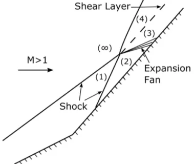
Figure 3.2: Labeled image of established flowfield for 25-55 double-cone. primary triple point of the main oblique shock and the bow shock. Over the span of the next 20µs the laminar nature of the structure breaks down.

The start of this breakdown is seen in Figure 3.4d where several changes to the flow field are seen to simultaneously occur. The wave which reflects off the shear layer breaks down into a series of repeating waves which convect downstream. The break-down progresses and after approximately 25µs no apparent structure is observed. Additionally we observe a series of waves behind the separated shock. In the videos these waves appear to emanate from the reattachment shock and oscillate between the separation shock and the reattachment shock. These oscillations in the reattach-ment shock persist for the remainder of the test. As time progresses the separation location moves upstream and reaches the test time location by 0.765 ms as seen in Figure 3.4f. As the separation shock moves forward the triple point formed by the intersection of the separation and bow shock moves downstream. This causes the transmitted impingement shock to move downstream as well as the size and shape of the post bow shock structure remains constant through the test. For this shot the test time reservoir pressure level was reached at 1.015 ms (accounting for the nozzle flow through time). Thus the separation has found a stable configuration before the

(45)

(a) t=0.24 ms (b) t=0.275 ms

(c) t=0.325 ms (d) t=0.395 ms

(e) t=0.46 ms (f) t=0.63 ms

(g) t=1.085 ms (h) t=1.415 ms

Figure 3.3: T5 25-55 H8-Re2 nitrogen double-cone startup process, Shot 2856. All times are referenced from primary shock endwall reflection. The viewing area is 42.7 mm×26.7 mm.

(46)

(a) t=0.230 ms (b) t=0.255 ms

(c) t=0.285 ms (d) t=0.290 ms

(e) t=0.430 ms (f) t=0.765 ms

(g) t=1.155 ms (h) t=1.440 ms

Figure 3.4: T5 25-55 double-cone H8-Re2 air startup process, Shot 2858. All times are referenced from primary shock endwall reflection.

(47)

reservoir pressure has stabilized.

The H8-Re2 carbon dioxide startup process is shown in Figure 3.5, shot 2875. Note that the shocks are rather difficult to see for this shot due to issues with focusing the camera from resetting up the shadowgraph system. The startup process is similar to the other two gas compositions. The primary difference is in the growth pattern of the boundary layer separation. The separation is initially small such that the separation shock does not interact with the leading oblique shock until 700µs. At this point the separation grows outward until it reaches its maximum size at 1.05 ms while simultaneously the nozzle reservoir experiences a local minimum in stagnation pressure. The stagnation pressure then rises slightly and levels off for approximately 400µs over which the measurements are made. As the pressure rises in the reservoir the boundary layer separation retreats slightly upstream and then remains steady. Through this process the structure of the shock-shock interaction remains constant, however the location of the triple point shifts due to the interaction of the separation shock with the leading oblique shock.

The double-cone startup process for the H8-Re6 nitrogen run condition is shown in Figure 3.6. The high and low pressure shots have the same general shock structure. At the start of the test the oblique and bow shock form at 260µs with the oblique shock reaching its established location at 320µs. The separation is initially not visible for this condition. It first appears 410µs after the test start and is initially located close to the corner. It grows to its established size over a span of 350µs where it remains for the remainder of the test. The separation shock for this condition does not intersect the leading oblique shock due to the smaller separation size. It also does not appear to strongly influence the triple point transmitted shock. There are no changes in the overall flow structure once the separation location stabilizes.

The double-cone startup process for the H8-Re6 air run condition is shown in Figure 3.7. The startup begins similarly to the H8-Re6 nitrogen condition in the time it takes for the oblique and bow shock to form and stabilize in position. The major difference from the nitrogen case is that the separation is observable from the beginning of the test and is located away from the hinge. Over the next 980µs the

(48)

(a) t=0.23 ms (b) t=0.35 ms

(c) t=0.56 ms (d) t=0.64 ms

(e) t=0.86 ms (f) t=1.05 ms

(g) t=1.20 ms (h) t=1.41 ms

Figure 3.5: T5 25-55 double-cone H8-Re2 CO2 startup process, Shot 2875. All times are referenced from primary shock endwall reflection.

(49)

(a) t=0.25 ms (b) t=0.29 ms

(c) t=0.32 ms (d) t=0.37 ms

(e) t=0.58 ms (f) t=0.86 ms

(g) t=1.19 ms (h) t=1.45 ms

Figure 3.6: T5 25-55 double-cone H8-Re6 nitrogen startup process, Shot 2862. All times are referenced from primary shock endwall reflection.

(50)

separation oscillates a distance of 5.8 mm to 8.8 mm away from the hinge. Through the remainder of the test the separation oscillates over a distance of less than 1 mm. Like the nitrogen case, once the separation reaches its test time location, no other changes in the shock interactions are observed.

The startup process for the 25-48 double-cone is examined next. A labeled shad-owgraph image of the important flow features for the 25-48 double-cone is shown in Figure 3.8. The shadowgraph images showing the flow startup are found in Fig-ure 3.9. All of the test conditions studied with the 25-48 double-cone admit very similar startup processes to one another so only the H8-Re2 air test condition will be examined here. Supersonic flow establishes over the model by 260µs with the completed formation of the fore and aft oblique shocks. The boundary layer separa-tion is also apparent at this time. Over the next 150µs the forebody oblique shock steepens and the separation location moves upstream. From this point on there are only small oscillations in the separation location and no movement of the forebody oblique shock. The remaining changes that the flow undergoes