Learning Robust and Discriminative Manifold Representations for Pattern Recognition

Theses 4-2016

Learning Robust and Discriminative Manifold Representations for

Learning Robust and Discriminative Manifold Representations for

Pattern Recognition

Pattern Recognition

sk3100@rit.edu

Follow this and additional works at: https://scholarworks.rit.edu/theses Recommended Citation

Recommended Citation

Kumar, Sriram, "Learning Robust and Discriminative Manifold Representations for Pattern Recognition" (2016). Thesis. Rochester Institute of Technology. Accessed from

This Thesis is brought to you for free and open access by RIT Scholar Works. It has been accepted for inclusion in Theses by an authorized administrator of RIT Scholar Works. For more information, please contact

Manifold Representations for

Pattern Recognition

by

Sriram Kumar

A Thesis Submitted in Partial Fulfilment of the Requirements for the

Degree of Master of Science in Electrical Engineering

Supervised by

Dr. Andreas Savakis

Department of Computer Engineering

Kate Gleason College of Engineering

Rochester Institute of Technology

Rochester, NY

April 2016

Approved by:

Dr. Andreas Savakis,

Primary Advisor, Department of Computer Engineering

Dr. Panos P. Markopoulos,

Committee Member, Department of Electrical Engineering

Dr. Raymond Ptucha,

Committee Member, Department of Computer Engineering

Dr. Sohail Dianat,

I would also like to dedicate this thesis to my mother

Smt. Rajeswari Kumar and sister Smt. Priya Karthik.

First and foremost, I would like to express my gratitude to my advisor Dr. An-dreas Savakis, for his guidance, patience, mentorship and encouragement in making this research possible. The Vision and Image Processing lab became my second home where I spent most of my time. I learnt a “looot” over the past year and had the opportunity to work on multiple projects. The door to his of-fice was always open whenever I ran into a trouble spot or had a question about my research or writing. And most of all I would like to thank him for “bearing” with my writing.

I would also like to thank Dr. Raymond Ptucha for his enthusiastic teaching in machine intelligence class and for serving as my thesis committee. I would also like to thank Dr. Panos P. Markopoulos for serving as a member of my thesis committee. I would like to thank the committee members for their valuable feedback and comments.

I would also like to thank my fellow lab mates Bret Minnehan and Matthew Johnson for their endless discussions, fun and banter that we had in the lab. Finally, I must express my very profound gratitude to my mother and my sis-ter for providing me with unfailing support and continuous encouragement throughout my years of study and through the process of researching and writ-ing this thesis. This accomplishment would not have been possible without them. Thank you.

Learning Robust and Discriminative Manifold Representations for Pattern Recognition

by Sriram Kumar

Face and object recognition find applications in domains such as biometrics, surveillance and human computer interaction. An important component in any recognition pipeline is to learn pertinent image representations that will help the system to discriminate one image class from another. These represen-tations enable the system to learn a discriminative function that can classify a wide range of images. In practical situations, the images acquired are often cor-rupted with occlusions and noise. Thus, a robust and discriminative learning is necessary for good classification performance.

This thesis explores two scenarios where robust and discriminative manifold representations help recognize face and object images. On one hand learning robust manifold projections enables the system to adapt to images across differ-ent domains including cases with noise and occlusions. And on the other hand learning discriminative manifold representations aid in image set comparison. The first contribution of this thesis is a robust approach to visual domain adap-tation by learning a subspace withL1principal component analysis (PCA) and

L1 Grassmannian with applications to object and face recognition. Mapping data from different domains on a low dimensional subspace through PCA is a common step in subspace based unsupervised domain adaptation. Subspaces extracted by PCA are prone to be affected by outliers that lead to noisy projec-tions. A robust subspace learning through L1-PCA helps in improving

perfor-mance. The proposed approach was tested on the office, Caltech - 256, Yale-A and AT&T datasets. Results indicate the improvement of classification accuracy for face and object recognition task.

The second contribution of this thesis is a biologically motivated manifold learn-ing framework for image set classification by independent component analysis (ICA) for Grassmann manifolds. It has been discovered that the simple cells in the visual cortex learn spatially localized image representations. Similar repre-sentations can be learnt using ICA.

linear subspaces. The efficacy of the proposed approach is demonstrated for image set classification on face and object recognition datasets such as AT&T, extended Yale, labelled faces in the wild and ETH - 80.

Acknowledgements ii Abstract v Contents vii List of Figures ix List of Tables xi 1 Introduction 1

1.1 Why is Domain Adaptation Important? . . . 3

1.2 Why is Image Set Comparison Important? . . . 4

1.3 Thesis Contributions . . . 5

1.4 Thesis Outline . . . 5

2 Unsupervised Subspace Learning 7 2.1 Dimensionality Reduction . . . 7

2.1.1 Principal Component Analysis . . . 9

2.1.2 L1Principal Components Analysis . . . 11

2.1.2.1 Fast Computation of Eigenvectors . . . 12

2.2 Manifold Learning . . . 14

2.3 Independent Component Analysis . . . 14

2.3.1 Whitening Transformation . . . 15

2.3.2 The Information Maximization Algorithm (Infomax) . . . 17

2.3.3 ICA-Architecture I : Independent Basis Images . . . 19

3 Grassmann manifolds 21 3.1 Grassmannian Geometry . . . 21

3.1.1 Grassmann Metrics . . . 23

3.2 Grassmann Kernels . . . 23

3.3 L1- Grassmann manifold . . . 24

3.4 Grassmann Manifold Learning with Independent Component Anal-ysis . . . 25

3.4.1 Biological Motivation Underlying the Learning Framework 26

4 Classification Techniques 27

4.1 Statistical Learning Theory. . . 28

4.2 Support Vector Machines. . . 29

4.3 Kernel Algorithms . . . 31

4.4 SVM with kernels . . . 31

4.4.1 Kernel Discriminant Analysis with Grassmann kernels . . 32

4.5 Sparse Representation Classification . . . 33

4.5.1 Grassmannian Sparse Representation in RKHS . . . 35

5 Application ofL1PCA to Domain Adaptation 37 5.1 Domain Adaptation . . . 37

5.2 Related Work . . . 39

5.2.1 Geodesic Subspace Sampling . . . 41

5.2.2 Geodesic Flow Kernel . . . 43

5.2.3 Subspace Alignment . . . 45 5.3 Experiments . . . 47 5.3.1 Datasets . . . 47 5.3.1.1 Office database . . . 47 5.3.1.2 AT&T database. . . 49 5.3.1.3 Yale-A database . . . 50

5.3.1.4 Datasets with domain shift . . . 50

5.4 Results&Analysis . . . 51

5.5 Statistical Significance Test . . . 62

6 Application of Perceptual Manifold to Image Set Classification 64 6.1 Image Set Classification . . . 64

6.2 Experiments . . . 65

6.2.1 Datasets . . . 66

6.2.1.1 Extended Yale Face Database . . . 66

6.2.1.2 Labelled Faces in the Wild (LFW) . . . 66

6.2.1.3 ETH-80 . . . 68

6.3 Results&Analysis . . . 68

6.4 Sensitivity Analysis . . . 70

7 Conclusion 75 7.1 Future Research . . . 76

2.3 Top two principal components computed from the given data . . 11 2.4 Two independent components and two principal components

over-laid on the data that is not Gaussian distributed. . . 15 2.5 Histograms of an imageset data before whitening is shown in

Figure 2.5a and after whitening is shown in Figure 2.5b. . . 16 2.6 Extracting statistically independent basis images under

architec-ture I. . . 17 2.8 Top to bottom 2.8a) ICA 2.8b) PCA . . . 20 5.3 Visual representation of the Geodesic Subspace Sampling (GSS)

on the Grassmann manifold between the source domain web-cam and target domain DSLR. The red and orange dots repsent subspaces corresponding to source and target domains re-spectively. The intermediate dots represent the intermediate sub-spaces along the geodesic path connecting the source and target domain. A domain invariant feature representation is obtained by concatenating the sampled subspaces. . . 41 5.4 Visual representation of the geodesic fow kernel (GFK) on the

Grassmann manifold between the source domain webcam and target domain DSLR. The red and orange dots represent the ba-sis vectors of the source and target domains respectively. The intermediate dots represent the intermediate basis vectors along the geodesic path connecting the source and target domain. A kernel matrix is implicitly learnt by integrating all the intermedi-ate subspaces, which transforms the source and target data into a high dimensional space, in which classification is done. . . 44 5.5 Visual representation of the Subspace Alignment (SA) between

the source domain webcam and target domain DSLR. The blue and red lines represent the basis vectors of source and target do-mains respectively. The transformation box M takes in both the basis vectors from the source and target domains and outputs a set of basis vectors that are aligned with the target domain’s basis. 46 5.6 Sample images from each domain 5.6a) Amazon 5.6b) DSLR 5.6c)

Webcam 5.6d) Caltech256. . . 48 5.7 Sample images in AT&T database 5.7a) Source domain 5.7b)

Tar-get domain. . . 49

5.8 Sample images in Yale database 5.8a) Source domain 5.8b) Target domain.. . . 49 5.9 Plot of adaptation accuracies versus number of subspace

dimen-sions as the number of images in target domain using GSS for office and Caltech - 256 databases. . . 56 5.10 Plot of adaptation accuracies versus number of subspace

dimen-sions as the number of images in target domain using GFK for office and Caltech - 256 databases. . . 57 5.11 Plot of adaptation accuracies versus number of subspace

dimen-sions as the number of images in target domain using SA for of-fice and Caltech - 256 databases. . . 58 5.12 Plot of adaptation accuracies versus number of subspace

dimen-sions as the number of images in target domain using GSS for AT&T database. . . 59 5.13 Plot of adaptation accuracies versus number of subspace

dimen-sions as the number of images in target domain using GFK for AT&T database. . . 59 5.14 Plot of adaptation accuracies versus number of subspace

dimen-sions as the number of images in target domain using SA for AT&T database. . . 60 5.15 Plot of adaptation accuracies versus number of subspace

dimen-sions as the number of images in target domain using GSS for Yale-A database. . . 60 5.16 Plot of adaptation accuracies versus number of subspace

dimen-sions as the number of images in target domain with NN using GFK for Yale-A database.. . . 61 5.17 Plot of adaptation accuracies versus number of subspace

dimen-sions as the number of images in target domain using SA for Yale-A database.. . . 61 5.18 Box-plots indicating 95% confidence intervals for classification

accuracy across different domain pairs. . . 63 6.4 The vertical axis denotes the number of images (in %) that were

corrupted by random sized occlusions. 6.4a) GPCA vs. GRAIL classification of occluded AT&T database using nearest neighbor classification. 6.4b) GPCA vs. GRAIL classification of occluded AT&T database using Sparse representation classification. . . 72 6.5 Indpendent components learnt from classes 1,2,3 and 4

respec-tively in the Extended Yale dataset. . . 73 6.6 Indpendent components learnt from one instance of each

5.1 Recognition accuracy (in %) with unsupervised Domain Adapta-tion using NN. (A: AMAZON, C: CALTECH, D: DSLR, W:

WE-BCAM). . . 52

5.2 Recognition accuracy (in %) with unsupervised Domain Adap-tation using SVM. (A: AMAZON, C: CALTECH, D: DSLR, W: WEBCAM). . . 53

5.3 Recognition accuracy (in %) with unsupervised domain adapta-tion using NN classificaadapta-tion for AT&T dataset. . . 54

5.4 Recognition accuracy (in %) with unsupervised domain adapta-tion using NN classificaadapta-tion for Yale dataset. . . 54

5.5 Recognition accuracy (in %) with unsupervised domain adapta-tion using SVM classificaadapta-tion for AT&T dataset. . . 54

5.6 Recognition accuracy (in %) with unsupervised domain adapta-tion using SVM classificaadapta-tion for Yale-A dataset. . . 54

6.1 Performance comparison on AT&T dataset with Training using first five images.Testing using last five images. . . 70

6.2 Performance comparison on extended Yale dataset based on 2-Fold Cross Validation (best performance reported for all the meth-ods).. . . 70

6.3 Performance comparison on LFW dataset. . . 70

6.4 Performance comparison on LFW dataset. . . 71

6.5 Performance comparison on ETH-80 dataset. . . 71

6.6 Performance comparison on occluded AT&T dataset based on three-fold cross validation repeated 20 times. . . 72

Introduction

The human brain is confronted with high dimensional multi-modal sensory data everyday. The task of visual recognition is performed effortlessly by the human brain by extracting only the pertinent information from the sensory data. Even in the presence of occlusion, recognition of objects and faces is done efficiently. Building a system to accomplish the task of visual recognition is not trivial. Challenges include recognition under occlusion, noise, unconstrained environments (a.k.a in the wild), variations in illumination and pose to name a few. Applications of interest include domains such as robotics, military, surveil-lance, entertainment and health-care to name a few.

The standard pipeline for a such a task starts with feature extraction followed by a statistical or machine learning algorithm to learn how to make decisions from examples and use that knowledge to classify or recognize the objects. The first task is to extract meaningful representations for the objects [1]. For appli-cations such as face and facial expression recognition, texture based features are used since they capture shape information and are invariant to illumina-tion variaillumina-tions. Popular texture descriptors include Local Binary Pattern (LBP) and Local Ternary Pattern (LTP) [2]. On the other hand for applications such

as object recognition, it is desired to extract features that capture local infor-mation such as edges and corners. Some popular descriptors include Scale In-variant Feature Transform (SIFT) [3] , Speeded Up Robust Features (SURF) [4] and convolutional features [5]. Another way of representing objects include

bags of features [6, 7] and feature encoding [8, 9] methods. In simple words, such a representation encodes the information in a histogram. The above men-tioned features are application specific and often parametric, thus require tun-ing of hyper-parameters to suit the data at hand. In thedeep learningfront, there has been a proliferous growth in feature learning. Deep networks have shown to perform feature extraction, dimensionality reduction and classification, and thus alleviating users from handpicking features and classifiers to be used [10– 12].

The features that are obtained from the feature extraction process are often high dimensional. Understanding such high dimensional data can be challenging as well as computationally demanding for any statistical or machine learning algorithm. It is advantageous to follow the feature extraction step with dimen-sionality reduction in the form of manifold learning [13]. Linear dimensionality techniques include Principal Components Analysis (PCA) and Linear Discrimi-nant Analysis (LDA) find a new subspace that spans the input data. Non-linear versions of manifold learning include Laplacian eigenmaps [14], ISOmetric fea-ture MAPping (ISOMAP) [15] and Locally Linear Embedding (LLE) [16]. These methods are referred to as feature embeddings. The above linear and non-linear dimensionality reduction techniques try to preserve some desirable property of the data in the reduced space such as variance, neighborhood information or reconstruction error. It has been shown that these manifold learning techniques are actually instances of Kernel Principal Component Analysis (KPCA) accord-ing to different kernel functions [17].

is efficient and discriminative [18, 19]. Grassmann geometry represents linear subspaces as points on the manifold. Grassmann kernelization embeds sub-spaces onto a projective space where distance computations can be effectively performed. Classical algorithms such as nearest neighbors, support vector ma-chines [20] and sparse representation based classification [21] can be performed on this projective space.

This thesis focuses on two problems in computer vision namely unsupervised visual domain adaptation and image set classification.

1.1

Why is Domain Adaptation Important?

Learning to ride a motorcycle is easier once a person masters how to ride a bicycle. This is because, both the activities are similar and the skills can be transferred. Such an adaptation task is called transfer learning. Visual domain adaptation is a specific case of transfer learning where the system tries to recog-nize the same object categories obtained from different domains such as a DSLR and webcam. The human brain can identify a car if it is shown on a television, a computer or on the road. When a system learns to identify an image of a car from a database acquired using a DSLR, it often fails to adapt itself when it tries to recognize an image of a car obtained from the internet. The process of adap-tation which comes naturally to humans is difficult to impart to a system. Re-cently subspace based techniques have gained popularity in domain adaptation [22–28]. Specifically, we study three subspace based domain adaptation meth-ods namely Geodesic Subspace Sampling [22], Geodesic Flow Kernel [23] and Subspace Alignment[24]. These methods perform principal component analy-sis to derive meaningful subspace representations. Although it is simple and intuitive, principal components are sensitive to outliers and often extract noisy projections even in the presence of one outlier and corrupts the representations

[29]. This is attributed to the formulation of the optimization problem under

L2 norm. To this end, principal components are extracted by performing op-timization under L1 norm since it is more robust to outliers. Object and face

recognition is performed where a model is learnt by extracting robust subspace representations from one domain and applied on another domain having the same object classes.

1.2

Why is Image Set Comparison Important?

The human eye is presented with rich visual data on a daily basis that is under constant flux. It is believed that the visual cortex models all the variations of an object on a manifold [30]. In image set classification, large amounts of data of a single object or person is available at hand over long periods of time with varia-tion in pose and illuminavaria-tion. It has found a myriad of applicavaria-tions in domains such as biometrics for security, military for surveillance and entertainment for face tagging to name a few. Characterizing such images as a manifold enables efficient modelling and circumvents the problem of “Curse of Dimensionality”. We derive meaningful representations using independent components analy-sis and learn a Grassmann manifold where we perform classification. Better representations are harnessed from image sets rather than a single image, as this helps in exploiting the underlying geometrical structure. The benefits of learning a manifold include dimensionality reduction and improved class sep-aration.

1.3

Thesis Contributions

The first contribution of this thesis is a robust approach to domain adaptation with applications to object and face recognition. The second contribution of this thesis is an algorithmic framework inspired by the human visual system called the perceptual manifold applied to the problem of image set classifica-tion. These contributions are summarised as follows:

• Robust domain adaptation

– Analysis and evaluation of three subspace based domain adaptation techniques Geodesic Subspace Sampling, Geodesic Flow Kernel and Subspace Alignment.

– Learning a robust subspace extraction usingL1norm to perform do-main adaptation.

• Image set classification

– Analysis and evaluation of Grassmann learning with kernels and sparse representation for image set classification.

– Proposes a biologically motivated framework for image set classifi-cation.

– Extending the proposed approach to incorporate sparse representa-tion based classificarepresenta-tion.

1.4

Thesis Outline

Following the introduction,Chapter 2presents the concept unsupervised sub-space learning. Classical techniques such as principal component analysis and

random projections are discussed. In addition, L1 principal component anal-ysis is also reviewed. This is followed by an overview of manifold learning. The chapter concludes with the discussion of independent component analysis.

Chapter 3introduces the Grassmann learning framework. This is followed by the description of different metrics and kernels defined on the Grassmann man-ifold. The chapter concludes with the discussion of robust and discriminative Grassmann learning using L1 principal component analysis and independent component analysis. Chapter 4 formally introduces the problem of learning with a statistical perspective. This is followed by an overview of support vector machines and its kernel extension. The chapter concludes with explanation of how discriminant analysis and sparse representation based classification can be performed on the Grassmann manifold. Chapter 5 introduces the problem of visual domain adaptation. An overview of different methodologies in the liter-ature is presented. This is followed by the discussion of three methods based on subspace learning namely Geodesic Subspace Sampling, Geodesic Flow Kernel and Subspace Alignment. The experimental protocol and datasets used in face and object recognition are then described. The chapter concludes with the dis-cussion of the results and analysis. Chapter 6introduces the problem of image set classification and current approaches to the problem. A new algorithmic framework to model image sets and perform classification by learning a Percep-tual manifoldis presented. This is followed by the biological motivation behind this algorithm. Experimental protocols and datasets used in experiments are then detailed. The chapter concludes with the discussion of the results and analysis. Chapter 7summarizes the findings and discusses possible extensions to pursue.

Unsupervised Subspace Learning

2.1

Dimensionality Reduction

FIGURE2.1: Visualization of toy data spread inR1,R2andR3.

Dimensionality reduction is the process of mapping the data from its high di-mensional image space to a lower didi-mensional subspace through some kind of transformation or mapping. Working with high dimensional data can be com-putationally challenging and thus some form of reduction in representation is needed. Images themselves are high dimensional. For example, an image

I ∈ R1000,1000_{pixels resides in a high dimensional image space having 1,000,000}

dimensions. There is a lot of redundant information since not all the pixels in the image contain useful information. The human visual system (HVS) is very

FIGURE 2.2: Conceptual illustration of mapping from a high dimensional spaceRDto a lower dimensional subspaceRm,m D

efficient at extracting discriminative image representations images and mod-elling them in a lower dimensional subspace [30]. Inspired by the working of the HVS, feature engineering has been an active research with the aim of ex-tracting information relating to textures [2], edges [31], corners [32]. However this causes additional increase in dimensionality. A common problem associ-ated with big feature spaces is the “Curse of Dimensionality” which was coined by Richard Bellman [33] in 1961. This phenomenon is illustrated in Figure2.1. It can be observed that as dimensionality increases, data samples become sparsely distributed and thus exponentially large amounts of data are needed with in-crease in dimensionality [34]. Another problem is that scalability of algorithms in higher dimensions [35]. The key reasons for pursuing dimensionality reduc-tion techniques can be summarized as follows:

– Computational complexity: Perform classification in a dimensionality re-duced space, as it decreases the load on the computation.

– Noise reduction: Mitigate the effects of noise and redundant information contained in the data and thus display the data in a compact space. – Visualization: Visualize the spread of data in two or three dimensions and

– Feature extraction: Harness better representations of the data in the lower dimensional space that promote discrimination and improve classification accuracy.

In this thesis we explore unsupervised subspace learning techniques to learn a transformation or mapping matrix. The idea of dimensionality reduction can be stated as follows: given the data X ∈ RD_{, estimate a mapping that transforms} the data to Rm, such that m < rank(D). The mapping is given by,Y 7→ RX, where R ∈ Rm,D_{. This process is illustrated in Figure 2.2. A comprehensive} review of linear dimensionality reduction technique is presented in [36].

We first start by describing Principal Component Analysis (PCA) which is a classic and common dimensionality reduction technique. In short, PCA finds a linear transformation matrix which minimizes the reconstruction error between the original data and the projected data in the least square sense, or equivalently finds a space that maximizes the variance in the data. This is followed by L1

principal component analysis which is a robust version of the standard PCA, since it tries to minimize the reconstruction under L1 norm. This formulation has no closed form solution but many optimal algorithms have been proposed to solve the problem [37]. We conclude this chapter by describing Independent Component Analysis (ICA), which is an extension of PCA that utilizes higher order statistics.

2.1.1

Principal Component Analysis

Principal Component Analysis (PCA) is a statistical technique that transforms a set of correlated variables into a set of linearly uncorrelated variables using an orthogonal transformation. It is a linear dimensionality reduction technique that projects the data from its original space into a new subspace that maxi-mizes the variance. LetX = [x1,x2, . . . ,xN] ∈RD,N denote the data matrix. We

assume that the data is mean subtracted, i.e. _N1 ∑N i=1

xi = 0. PCA can be formu-lated as a minimum reconstruction error problem, wherein the goal is to find the orthonormal projection matrix that best minimizes the reconstruction error, in the mean square sense. LetR∈ RD,m _{an orthonormal matrix having rankm.} The PCA problem is defined as:

E2 =kX−RVk2_F (2.1)

whereV ∈ Rm,N _{andV = R}T_{X. This problem can be reformulated as a} projec-tion maximizaprojec-tion problem by solving,

RL2 =arg maxTr[R

TXXTR] (2.2)

where, Tr(.) denotes the trace of a matrix. Since kAk2

F= Tr(ATA), Equation (2.2) can be re-written as,

RL2 =arg maxkX

T_Rk

2. (2.3)

The above problem can be solved by eigenvalue decomposition and the top m

eigenvectors ofXXTmaximize the variance in the data. Alternatively, principal components can be computed using singular value decomposition (SVD). An illustration of PCA is shown in Figure2.3. The data is generated by sampling from a multivariate Gaussian distribution. The top two principal components are overlaid on the data to show the principal directions. We see that the leading principal component is in the direction of maximum variance of the data. PCA is a standard tool in any machine learning pipeline due to its simplicity and ef-fectiveness. However, in practical situations, data at hand is contaminated with noise and outliers. PCA is sensitive to noise and can lead to noisy components [38]. In the next section, a robust approach is described to learn components in

FIGURE2.3: Top two principal components computed from the given data.

the presence of outliers.

2.1.2

L

Principal Components Analysis

The problem with PCA formulation under L2-norm approach is sensitive to outliers [39]. Even a single outlier can affect the direction of the principal com-ponent. In order to make it robust, the problem is formulated under L1norm.

Under the L1formulation, Equation (2.1) becomes,

E1 =kX−RVk1. (2.4)

And the projection maximization formulation presented in Equation (2.3) be-comes,

RL1 =arg maxkX

T_Rk

1. (2.5)

As a consequence of this reformulation, Equation (2.4) and (2.5) are no longer equivalent under L1constraints. The optimal solution to the above L1problem

is NP-hard [37]. It was proved that [39] the optimal solution for L1 principal component is given by,

rL1 =

Xbopt

kXboptk2 (2.6)

whereboptis a binary vector having lengthNand entries from{−1,+1}. It was also shown that in [39], kXTrL2k1 =kXboptk2andboptcan be solved by,

bopt =arg maxkXboptk2 =arg maxbTXTXb (2.7)

A fast computation of principal components was presented in [29] and is oerviewd in the next section.

2.1.2.1 Fast Computation of Eigenvectors

In [29], a fast computation of one principal component was proposed based on bit flipping. We give an overview of the algorithm below. A binary vector is initialized from the column of the covariance matrix of the input data. Then the bits that contribute negatively to the projection energy are flipped. This process is repeated on every column of the covariance matrix and the optimal binary vector is converted into an eigenvector. The first step is to identify the bits that negatively affect the projection energy. The quadratic form of Equation (2.7) is given by, bTXTXb= Tr(XTX) +

∑

∑

In order to identify the bits that have negative effect on the aggregate maximum, a parameterαis defined as,

αi,±4bi

∑

bj XTX

Algorithm 1Computation ofL1principal component [29]

1: Input: X ∈RD,N _{data matrix} 2: [B]:,n ←single bit flippping

Xj,sign[XTX]_:ni

3: c← argmaxi[BTXTXB]i,i

4: Return: rˆL1 =X[B]:,c/kX[B]:,ck2

Function: single bit flippping

1: Input: X ∈RD,N data matrix andb ∈ {±1}N

2: Repeat: 3: αi ← bi ∑j6=ibj[XTX]i,j ∀i∈ 1, . . . ,N 4: i f(v<0)bp ← −bp;else, EXIT 5: Return: b

The bits that negatively contribute can be found using Equation (2.9) and are flipped. Thus by findingbopt, Equation (2.6) can be used to determine the cor-responding eigenvector. An extension of this approach to multiple principal components by using a greedy strategy was presented in [38,40].

xupdate_i = xi−r(rTxi)∀i ∈ {1, . . . ,N} (2.10)

After the first principal component is computed, the contributions of that bit from all the data is removed and the above Equation (2.10) is updated. The bit flipping algorithm (even for one principal component) does not guarantee optimal solution but the principal components are orthonormal. This process is repeated until the required number of components or eigenvectors are com-puted. The steps involved in the fast computation of L1 eigenvectors are

de-tailed in [29, 38]. For completeness we present the psuedocode of the bit flip-ping algorithm for fast computation ofL1principal component in Algorithm1.

2.2

Manifold Learning

A manifoldMis a topological space that is locally homeomorphic tom dimen-sional Euclidean space Rm, where mis the dimensionality of the manifold. A topological spaceX is called locally Euclidean if there is a non-negative integer

dsuch that every point inX has a neighborhood which is homeomorphic to the Euclidean space orRd. Homeomorphism is a function that preserves the local structure between topological spaces. In computer vision and machine learning applications, manifolds are often referred as image or signal manifolds which are subsets of a larger space. Manifold learning algorithms fall under non-linear methods for dimensionality reduction. They assume that the data is embedded on a non-linear manifold in high dimensional space. These low dimensional manifolds are embedded inRDas a non-linear surface. The mapping from high dimension to low dimension is estimated in a way that the geometrical structure is preserved as much as possible. Most of the manifold learning techniques in-volve constructing an adjacency graph based on some metric distance. A com-prehensive review of various manifold learning techniques including Laplacian eigenmaps [14], ISOmetric feature MAPping (ISOMAP) [15] and Locally Linear Embedding (LLE) [16] are discussed in [41].

2.3

Independent Component Analysis

Independent Component Analysis (ICA) is a generalization of PCA that is sen-sitive to higher order statistics [42]. We consider the signal x ∈ RN_{, x which} represents observations and can be written as a linear combination of the mix-ing matrix Aand source signals:

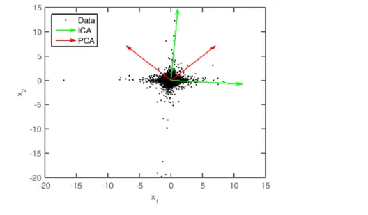
FIGURE 2.4: Two independent components and two principal components overlaid on the data that is not Gaussian distributed.

wheres∈ RN _{is the unknown source signal, assumed to be independent, andx} is the observed mixture of signals. The mixing matrix Ais invertible. The ICA algorithm tries to estimate the matrix A, or equivalently the separating matrix

W ∈ RN,N _{(Section2.3.2), based on the above assumptions and knowledge of} observationsxas follows,

U =Wx =W(As) (2.12)

Figure 2.4 shows an example where the ICA correctly identifies the compo-nents, in contrast to PCA, when the data is not Gaussian distributed. The steps involved in the process are described next.

2.3.1

Whitening Transformation

The retina in the eye tries to remove redundancy in the visual cortex [43]. This is achieved by transforming the visual information into a statistically indepen-dent basis by a process called whitening transformation. On average, natural

(A) (B)

FIGURE 2.5: Histograms of an imageset data before whitening is shown in Figure2.5aand after whitening is shown in Figure2.5b.

images follow1/f law in the frequency domain. When 2D Fourier transform is applied on a natural image, the magnitude of each component decreases as the frequency component increases. It could be that the human visual system re-duces the redundancy in information by reducing the magnitudes in frequency domain. Consequently it was shown in [44] that this corresponds to transform-ing the input data into a new basis in a way that they are uncorrelated. To speed up the process of ICA learning, the observations are preprocessed by whitening. This essentially removes correlation and reduces the dimensionality.

We start by centering our data. Let X = [x1, . . . ,xi, . . . ,xc] ∈ RD,N, i= 1, . . . ,c, denote the data samples of dimensionD, where Nis the total number of sam-ples and c is the total number of classes. The data is centered by subtracting the mean as, Xe = X−M(X), whereM(X) = _N1

N

∑

n=1

xn.The whitening transfor-mation matrix is obtained by performing the eigenvalue decomposition on the covariance matrix,

COV(Xe) = ΓΛΓT (2.13)

whereCOV(X) = _N1XeXeT,Γis the matrix containing the eigenvectors ofCOV(Xe) and Λ is the diagonal matrix of eigenvalues. It has been shown that in addi-tion to removing correlaaddi-tion among components E[XeXeT] = I

, the whitening transformation helps the convergence of the ICA algorithm and also improves

FIGURE2.6: Extracting statistically independent basis images under Architecture I.

performance in applications. The histograms before and after whitening trans-formation for a sample image set from AT&T dataset is shown in Figure2.5The whitening transformation is given by,

W =Λ−0.5ΓXe (2.14)

After performing PCA, only the top components were retained such that they account for at least 99% of the variance. Mathematically this can be state as,

m ∑ i=1 λi D ∑ i=1 λi ≥0.99 (2.15)

2.3.2

The Information Maximization Algorithm (Infomax)

To compute the independent components we use the Infomax algorithm pro-posed by Bell & Sejnowski [45]. Other methods for computing the independent components are presented in [46, 47]. The goal of the Infomax algorithm is to

maximize the mutual information1 between the input and the output of a sin-gle layer neural network. This algorithm was developed based on the idea that maximum information is transferred when a non-linear function (e.g. logistic function) is the same as the cumulative distribution function of the independent components. Let the outputs of the neurons be given asY = g(U), wheregis a mapping function that takes in an input and outputs value in the interval[0, 1]. The logistic function is defined as,

gi(U) = 1

1+e−U (2.16)

The variablesU1, . . . ,Unare linear combinations of inputs and can be thought of as pre-synaptic activations ofn-neurons. Similarly, the output variablesY1, . . . ,Yn are post-synaptic activations. The output values are bounded between [0, 1] by the logistic activation function. The learning algorithm was derived in [45] which maximizes the mutual information between inputXand outputYof the neural network. This is achieved by maximizing the entropy of output with respect to the weight by performing gradient ascent. This is equivalent to max-imizing the mutual information betweenXandYof the network. The gradient update is given as,

∆W ∝∇_WH(Y) = (WT)−1E(Y0XT) (2.17) whereY_i0 = g

00

i(Ui)

g0_i(Ui), is the ratio of the second and first derivative of the activation

function. In [48], an efficient natural gradient based learning was proposed to avoid the inverse computation of the weight matrix. This can be achieved by the multiplication ofWTW. The learning rule based on the natural gradient is given as,

∆W ∝∇_WH(Y)WTW = (I+Y0XT)W (2.18) 1_{It represents the mutual dependence between the two quantities. It is defined asI(X;Y) =} ∑y∈Y∑x∈X= p(x,y)log _pp_(x(x_)p,y₍)_y)

FIGURE2.7: Extracting statistically independent basis images under Architec-ture I.

In this work we used the logistic function, as it was shown to produce optimal filters. For convergence of the algorithm the learning rate was annealed slowly [45].

2.3.3

ICA-Architecture I : Independent Basis Images

In [49], two ICA architectures were proposed with applications to face recog-nition. In this thesis we utilized Architecture I to compute the independent components, which produces statistically independent basis images. Under this architecture, each face is considered as a random variable and its pixels as the observations. The data matrixXconsists of faces formed by a linear com-bination of independent basis images S and a mixing matrix A. In Figure2.6 a pictorial representation of the algorithm is shown. The ICA algorithm com-putes the matrixW, which recovers the independent basis images represented as the rows of matrixU. Before applying the ICA algorithm, PCA is performed on the data. This is beneficial for two reasons: (a) decorrelation of the data, which essentially removes the dependencies on second order statistics, or pair-wise dependencies, in the data; and (b) Reduced computational complexity due to dimensionality reduction. LetUbe the matrix of dimension(D,m)be the top

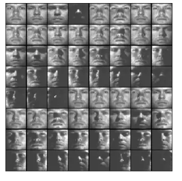
meigenvectors ofΓ(Equation2.13). The input to the ICA algorithm isUT. The basis images are obtained by multiplying the weights withX, i.e. WX[50]. Fig-ure 2.7 summarizes this process. Sample basis images learned from ICA and

PCA are shown in Figure 2.8. In the next chapter we introduce the concept of Grassmann manifold learning and how linear subspaces such as PCA and ICA can be used to construct a Grassmann manifold.

(A)

(B)

Grassmann manifolds

3.1

Grassmannian Geometry

A Riemannian manifold is smooth and differentiable manifold that extends the notion of Euclidean distances to non-flat spaces. Grassmann manifolds are a special class of Riemannian manifolds, as they are endowed with similar structure, which enables the computation of distances between points on the manifold through geodesics [51]. The geodesic distance between two points

x,y ∈ Mdenoted by dM(x,y) is the smallest distance between the two points

on the manifold. Subspaces are a special class of Riemannian manifolds [52]. The set ofmdimensional linear subspaces inRDis represented as pointG(m,D) on the Grassmann manifold [19]. Figure 3.1 shows two subspaces represent-ing classes in the high dimensional Euclidean space and their mapprepresent-ing on the Grassmann manifold, represented as two points which correspond to linear subspaces for each class respectively. This Grassmann structure enables an effi-cient way to model and compare image sets [53]. A point on the Grassmannian is represented as a matrix of dimension (D,m)whose columns span the same

FIGURE3.1: A conceptual representation of the Grassmann manifold. On the left, two image sets are described by linear subspaces in image spaceRD. On

the right, the subspaces are mapped as points on the Grassmann manifold.

subspace. The principal angle between two orthonormal matrices is defined as follows: cosθk = max p∈span(Y1) max q∈span(Y2) p_kTqk s.t.kpk2 =1,kqk2 =1 pT_kpi =0,qT_kqi =0,i =1, . . . ,k−1 (3.1)

The principal angles can be computed by the SVD of(Y₁TY2)asY₁TY2=UcosΘVT

whereU = [p1, . . . ,pm],V = [q1, . . . ,qm], andcosΘ=diag(cosθ1,cosθ2, . . . ,cosθm). AngleΘtakes values in the range ofθi =1 :m ∈ [0,π₂]. The principal angle can be viewed as a measure of correlation between the subspaces. A small value of θ implies that the subspaces are highly correlated and vice-versa. In order to measure the distance between the points on the manifold, valid distance met-rics are defined on the manifold. One such metric is the projection metric, which is the most commonly used in literature. The projection metric is a measure of distance between two points on the manifold and is defined in terms of the principal angles as,

d_Proj(Y1,Y2) = m− m

∑

3.1.1

Grassmann Metrics

In addition to the projection metric, there are other distance metrics defined on the manifold and these were explored in [18,20]. We list out the other distance metrics expressed in terms of principal angles below in Equations (3.3) through (3.6). Binet−Cauchy: d(Y1,Y2) = m−

∏

max correlation : d(Y1,Y2) = (1−cos2θ1)

1

2 (3.4)

min correlation: d(Y1,Y2) = (1−cos2θm)

1 2 (3.5) Procrustes: d(Y1,Y2) =2 m

∑

3.2

Grassmann Kernels

Kernel functions can be used as a method for similarity measurement. A ker-nel function maps the data from the original space into a reproducible kerker-nel Hilbert space (RKHS), a high dimensional space (possibly infinite) with inner productsh·,·i. With the aid of these kernel functions statistical classifiers such as a SVM can be used. There are various kernels used to induce isometric embed-dings that map the points from the Grassmann manifold to Hilbert spaces [54]. Intutively, “isometric embedding” maps Riemannian manifolds to Euclidean like spaces. The two common kernels used on the Grassmann manifold are pro-jection and Binet-Cauchy kernels. Amongst the two, the propro-jection kernel has shown to be the most effective [18] in terms of classification. LetY1,Y2 ∈ R(D,m)

FIGURE3.2: Constructing the Grassmann manifold from the original space by extracting linear subspaces.

on the Grassmannian is defined as,

KProj(Y1,Y2) = tr[(Y1Y1T)(Y2Y2T)] = kY1TY2k2F (3.7)

KBC(Y1,Y2) = det(Y1TY2Y2TY1) (3.8)

In Figure3.2, a conceptual flow is presented to construct the Grassmann man-ifold. In order to map the data from the original space onto the Grassmann space, the data samples from each class are first grouped together and then lin-ear subspaces are extracted for each class. On the Grassmann manifold, the linear subspaces are represented as points. There are multiple ways to extract subspaces from the data. In the next section, we detail two methods namely,L1

principal component analysis and independent component analysis for extract-ing subspaces.

3.3

L

- Grassmann manifold

In an unsupervised setting the most common method for subspace generation is the principal component analysis (PCA). PCA tries to find projections pointing in the direction of maximum variance by minimizing the mean squared error as given in Equation (2.3). The apparent problem in this approach is that the

method lacks robustness to outliers and noise, while trying to find the projec-tion along the direcprojec-tion of highest variance. This leads to finding projecprojec-tions in the direction of noise, which is not desirable [23,38]. In order to obtain a robust subspace that is less susceptible to noise or outliers, we utilize the L1-PCA to

obtain the subspaces. The L1-PCA has shown promising results in face

recog-nition with noise [38]. L1 Grassmannian [55] approach for subspace mapping

will be robust to the noise that may occur while mapping the subspace on the Grassmann manifold.

3.4

Grassmann Manifold Learning with Independent

Component Analysis

An important step in constructing the Grassmann manifold is the subspace con-struction. We propose a robust and discriminative approach to the problem of subspace learning by constructing the Grassmann manifold based on indepen-dent component analysis. We then utilize sparse representation classification in kernelized space using kernel embedding [21]. Figure 3.3 shows a flowchart overview of the proposed approach. The first step is image preprocessing, which involves cropping, scaling, centering and whitening the data. Then the images available in each class are used to form a subspace using independent component analysis and each subspace is mapped to a point on the Grassmann manifold. The process of kernelization using projection kernel is used to map to a Hilbert space where classification is performed with discriminant analysis or sparse representations based on minimum reconstruction error. It is notable that this framework allows image set comparisons, such as when multiple im-ages are available for use in face and object recognition.

FIGURE 3.3: Proposed algorithm for image set recognition using perceptual manifold.

3.4.1

Biological Motivation Underlying the Learning Framework

The human visual system is confronted with high dimensional visual infor-mation, but has the ability to extract only perceptually pertinent features [30]. These features intrinsically lie on a low dimensional space. The biological inspi-ration underlying our learning framework is twofold: (i) the basis functions ex-tracted by independent component analysis resemble Gabor-like filters, which closely model the responses of V1 simple cells [45]. These filters are spatially localized and exhibit separate high-order dependencies. Moreover, the high order statistics contain image phase information. (ii) The manifold hypothesis states that high dimensional data resides in a low dimensional manifold em-bedded in a Euclidean space. Once the visual system extracts the features, they are embedded on a perceptual manifold that characterizes the intrinsic dimen-sionality of the data [56]. We model this process by utilizing independent com-ponent analysis. This process is summarized in Figure3.3. In the next chapter we give a statistical overview of classification problem and discuss how pattern recognition can be performed on the Grassmann manifold.

Classification Techniques

Today in the age ofBig Data, there is unprecedented access to a plethora of vi-sual data. The ability to interpret, and discern the data at hand is a challenging task. The problem of classification deals with assigning labels to the data based on their attributes and prior examples. The classification problem can be stated as follows: We have access to a collection of data called thetraining setfor which the class labels are given. In the case of visual data, we are given a set offeatures

which have been engineered from the data and contain meaningful informa-tion about the data. This particular setting is termed supervised classification. Methods such ask-nearest neighbors [57] and support vector machines [58] fall under this category. With the available information at hand a machine learning or statistical algorithm is used to learn a model by providing examples. This stage is known as training phase. During the testing phase an unknown test sample is given to the model and model assigns a label. In the next section, we introduce the problem of pattern recognition with a statistical perspective.

4.1

Statistical Learning Theory

The problem of learning can be understood under a statistical learning frame-work of minimizing expected loss function using observed data. The learning problem is that of choosing the function f(x,α∗) from the given set of func-tions f(x,α),α ∈ Ωthat predicts the input dataxbest. Given a training dataset that is a set of n random observations [x1, . . . ,xn] and their associated labels [y1, . . . ,yn] that are independently identically distributed (i.i.d) according to some unknown probability distribution function, p(x,y) = P(x)P(x|y).

In the risk minimization problem, the indicator function f(x,α)is chosen as the best approximation to the response y out of all possible functionals. The loss function given by L(y, f(x,α)) is the measure of response between the differ-ence y to an input x and the output of the functional f(x,α) provided by the machine learning algorithm. The expected value of the loss function is given as,

R(α) = Z

L(y, f(x,α))dP(x,y) (4.1)

The goal is to find the function f(x,α∗) which minimizes the risk R(α) over all the possible functions f(x,α),α ∈ Ω when the joint probability distribu-tionP(x,y)is unknown and only the information in the training data is known Equations (??). The problem of pattern recognition can be defined as follows: Let the indicator function be given as f(x,α),α ∈ Ωwhich takes only two val-ues 0 and 1. Let the output be y which also takes two valuesy = {0, 1}. The loss-function is defined as,

L(y, f(x,α)) =        0, y= f(x,α), 1, y6= f(x,α). (4.2)

error. The problem, therefore, is to find the function which minimizes the prob-ability of classification errors, when the joint probprob-ability P(x,y) is unknown, but the training data is given. In the subsequent sections, supervised classifica-tion techniques and their kernelized versions are over viewed.

4.2

Support Vector Machines

FIGURE4.1: An optimal hyperplane separating the two classes represented as “+” (red) and “−” (green) respectively with a maximal margin. The support vectors represented by data inside the circle help in finding the optimal

hyper-plane.

The support vector machine (SVM) learning algorithm [58] is one of the most widely used algorithms for problems in pattern recognition. It is popularly know for its kernelized version. It achieves high performance and has well founded concepts from statistical learning theory [59]. Given an unknown pat-tern x, the SVM assigns a class label y(x) = ±1 by applying the discriminant function ˆy(x) = wTΦ(x) +b. The functionΦ(x)is a feature mapping function. The input patternxis mapped into the feature space using the functionΦ. The parameterswandbdenote the parameter vector and offset respectively, and are learned by the algorithm using the labeled training data (x1,y1), . . . ,(xn,yn). SVM is often referred as a large margin classifier, i.e. if the training data is

linearly separable then the SVM algorithm finds an optimal hyperplane that separates the two classes by maximizing the margin as much as possible. A vi-sualization of an optimal hyperplane learnt by SVM separating the two classes denoted by “+” and “−” is shown in Figure 4.1. The support vectors are rep-resented with a circle and help in constructing the margin. The optimization problem associated with the above problem is mathematically given as,

minimize w F(w,b) = 1 2w 2 subject to∀i yi(wTΦ(xi) +b)≥1 (4.3)

The above optimization problem can be solved by using Lagrange multipliers. The dual of the Equation (4.3) is given as,

maximize α D(α) = n

∑

∑

The objective function given in Equation (4.4) is computationally easier to solve. The term α denotes the weights and y ∈ {+1,−1} denotes the ground truth. Once the weightsα∗ are computed, the test point can be classified as,

ˆ y(x) = w∗Tx+b∗ = n

∑

4.3

Kernel Algorithms

Linear methods for classification are efficient when the data is linearly sepa-rable. But when the data has a non-linear structure, which is often the case, kernels provide an efficient way to capture the non-linearity in the data. The training data points can be mapped into high dimensional space, possibly infi-nite dimensional, that can capture the complex non-linear pattern in the data. Equation (4.4) involves computing the dot products between the input patterns. Alternatively, this dot product operation can be performed in an unknown fea-ture space using a kernel function Φ without explicit mapping into that fea-ture space. In [60], kernel function denoted by K(x,x∗) = Φ(x)TΦ(x∗) was proposed that computes the dot product in some unknown high dimensional space [61]. For a function to be a valid kernel function it must satisfy certain properties such as positive semi-definiteness and Mercer’s theorem [62].

4.4

SVM with kernels

The kernelized version of SVM is a powerful algorithm and often achieves state of the art classification. The dot product in Equation (4.4) can be replaced by a kernel function as,

maximize α D(α) = n

∑

∑

whereKij =K(xi,x∗_j)is the kernel matrix. Now, a test point can be classified as,

ˆ y(x) = w∗Tx+b∗ = n

∑

A commonly used kernel is the radial basis function (RBF) which was inspired from artificial neural networks (ANNs). For two patterns x and x0 the RBF kernel is defined as,

K(x,x0) =e

−kx−x0k

2σ2

. (4.8)

4.4.1

Kernel Discriminant Analysis with Grassmann kernels

Using the kernels defined in Section3.2, kernelized versions of classifiers such as discriminant analysis [63] can be obtained. Linear discriminant analysis (LDA) is a supervised dimensionality reduction and classification technique that finds projections to maximize the class separation by maximizing the ratio of between-class to the within-class scatter. This ratio is termed as the Rayleigh quotient. Let[x1,x2, . . . ,xN]be the data vectors and[y1,y2, . . . ,yN]be the corre-sponding class labelsyi ∈ {1, . . . ,C}respectively. We defineµc = _N1_c ∑{i|yi=c}xi

be the mean of class c and µ = _N1 ∑ixi be the total mean respectively. Let Nc andNbe the number of samples in each class and total number of samples. The LDA algorithm tries to maximize the Rayleigh quotient given by,

L(W) = |W T_S bW| |WT_S wW|. (4.9)

The between classSb and within classSc scatter matrix is defined as,

Sb = _N1∑Cc=1Nc(µc−µ)(µc−µ)T Sw = _N1∑C_c=1∑i|yi=c(xi−µc)(xi−µc)

T

(4.10)

The optimal projection matrix W is obtained from the largest eigenvector of

S_w−1Sb. The rank ofSw−1Sb isC−1, whereC is the number of classes. The data projected onto the space spanned byWachieves dimensionality reduction and

class discrimination. By using the kernel trick, the LDA algorithm can be ker-nelized [64]. Since the kernels defined on the Grassmann manifold are valid kernels and satisfy Mercer’s theorem, points from the Grassmann manifold can be mapped to a Hilbert space. The feature map is defined as,φ : G 7→ H. The Rayleigh quotient becomes,

L(W) = |W T_ΦT_S bΦW| |WT_ΦT_S wΦW| = |W T_ΦT_(V−1 N1T_N/N)ΦW| |WT_(Φ(I N −V)Φ+σ2IN)W| (4.11)

where Φis the kernel matrix, 1N is a vector of length N, V is a block diagonal matrix whose c-th block is the uniform matrix 1Nc1

T

Nc/Nc and σ 2_I

N is a regu-larization term. The algorithm of Grassmann Discriminant Analysis is given in [18].

4.5

Sparse Representation Classification

Sparse representations (SR) are inspired by studies on selective neurons firing to a stimuli such as images. Studies suggest that this is a phenomenon occur-ring in the visual cortex [65]. The idea of SR is to represent a signal by a set of sparse coefficients. Sparse in this context means that the coefficient vector has very few non-zero values. In the field of compressive sensing (CS) sparse representation theory has been very successful for signal reconstructions from very few samples. The SR framework has also been shown to be discriminative and robust to outliers. The sparsity and robustness stems from the fact that the optimization problem is formulated under L1 norm. In [66], SR was used for robust recognition and was shown to produce huge improvements in classifi-cation performance.

SR is closely tied to dictionary learning. Often a dictionary is “overcomplete” meaning that there are more samples than dimensions of the data. It has been

shown that learning a dictionary from the data can help in harnessing better sparse coefficients [67]. Recently SR based classification has been used in con-junction with manifold learning [68]. By using graph-embedding techniques the local geometry of the data and neighborhood information can be preserved. Mathematically the SR problem can be formulated as follows: Given a matrix

X = [X1|. . .|XC] ∈ RD×N, where C is the number of classes, N is the total number of samples D is the dimensionality and X which we will call as the dictionary. The dictionary X, is said to be overcomplete if N D. A test sampleycan be represented using the atoms in the dictionary as,

y =Xα (4.12)

whereα0∈ Rn is a sparse coefficient vector corresponding to the test sampley.

The sparse coefficient harnessed for sampleyhas non-zero entires correspond-ing to the cth class and zero elsewhere. In order to obtain a sparse solution, Equation (4.12) can be reformulated underL1norm as,

ˆ

α =arg min

α

kαk1 s.t.y =Xα (4.13)

where kαk1 = ∑i|α|. The L1 minimization problem promotes sparsity in the solution [69]. The problem presented in Equation (4.12) can be solved by pos-ing it as a LASSO (least absolute shrinkage and selection operator) regression problem as,

ˆ

α=arg min

α

kXα−yk22+λ|α|1 (4.14)

whereλis L1 norm regularization term that controls the amount of sparsity in

the solution. The solution may be obtained using orthogonal matching pursuit (OMP) [70] or least angle regression (LAR) [71]. In this thesis we solved the above problem in a least squares setting using the SLEP toolbox [72]. Given the

sparse coefficient ˆα for a test sample, images can be classified based on mini-mum reconstruction error [66]. The minimum residue for a classcis given by,

r∗ =arg min i=1:c

kXαˆi−yk2 (4.15)

4.5.1

Grassmannian Sparse Representation in RKHS

Algorithm 2Classification using Grssmannian Sparse Representation [21]. 1: Input: Ktrain,Ktest

2: Solve theL1minimization problem in Equation (4.13)

3: α∗ = arg min

α

kKtrainα −Ktest(i)k2₂ + λkαk1 s.t. Ktest = Ktrainα,i = (1, . . . ,Ntest)

4: Compute the residuals,r∗_i =arg min i=1:c

kKtest −Ktrainδi(α∗)k2₂ fori = 1, . . . ,C where,δi(α∗)is a vector whose non-zero elements corresponds to elements in class i

5: Return: predicted class label(Ktest) =arg minri(Ktest)

In this section we present the SR based classification on the Grassmann man-ifold. Following [21], we incorporate sparse representations in RKHS using kernelization. We construct the projection kernel matrix for the training sub-spaces: Ktrain ∈ R(Ntrain,Ntrain)_{, whereN}

train is the number of training subspaces, each one corresponding to a different class. This forms our dictionary. In a similar way we construct the projection kernel matrix for the test subspaces

Ktest ∈ R(Ntrain,Ntest)_{, where N}

test is the number of training subspaces. The SR problem is RKHS is given as,

α∗ =arg minkKtrainα−Ktest(i)k2₂+λkαk1 s.t. Ktest =Ktrainα,i = (1, . . . ,Ntest)

(4.16)

Under this setting, image set comparisons are possible, as each atom in our dictionary is a subspace corresponding to one class. We present the details for the Grassmannian Sparse Representation based classification in Algorithm

2. Sparse representation classification on Grassmann manifolds was used to achieve discrimination and robustness in classification. In Figures 4.2and 4.3, we show the sparse coefficients and the residual errors for a test subspace from AT&T and Yale database respectively. Figures4.2and4.3illustrate that the test subspace corresponds to one particular class subspace based on the residues. In the subsequent chapters, applications of robust Grassmann manifold for vi-sual domain adaptation and perceptual manifold learning for image set classi-fication presented.

(A) (B)

FIGURE4.2: Sparse coefficients harnessed using Grassmann ICA based SR and residual error for a sample class from AT&T database.

(A) (B)

FIGURE4.3: Sparse coefficients harnessed using Grassmann ICA based SR and residual errorr for a sample class from extended Yale database.

Application of

L

1

PCA to Domain

Adaptation

5.1

Domain Adaptation

FIGURE 5.1: Sample images across different categories from domains DSLR, amazon and webcam.

In practical machine learning problems, the data presented at test time is differ-ent from that the data used to train the classifier. In Figure 5.1sample images from three different domains namely DSLR, amazon and webcam are shown. The shift in domain is apparent by viewing these images. They vary in illumi-nation, resolution and pose. The three domains have the same object categories,

but contain visually dissimilar images. The process of adaptation comes natu-rally to humans, but it is hard to achieve for the computer. A model is typically learnt by the classifier such that it performs satisfactorily on the training data and can classify a similar test sample from the same dataset. However, when a test sample from a different dataset is applied to the classifier, it often fails to classify correctly. This may be attributed to the fact that the model is biased on the particular training dataset [73]. Torralba et al. [73] showed that the classifier learns something unique to each dataset. Their results pointed out that, each dataset has a distinct inherent bias or idiosyncrasy that causes the classifier to learn a biased model. This often results in poor cross-dataset generalization. The problem we address here is called visual domain adaptation, which falls under the category of transductive transfer learning where the train and test data have the same object categories but the domain shift is unknown [74]. One of the main problems in visual domain adaptation is that the nature of the domain shift is unknown. This raises the question of what is the best feature representation for a domain. Ben-David et al. [75] presented a theoretical anal-ysis indicating the choice of features representing the domains is such that the divergence1between the distributions in the feature space is minimized. In or-der to improve on the state of the art, algorithms are tuned towards a particular dataset. Despite being successful, the same algorithm may not perform as well on a different dataset. Thus we need a robust system that is able to perform rea-sonably well on any dataset without being idiosyncratic towards any particular one. Although this is desirable, it is hard to achieve.

There have been several approaches proposed to tackle this problem [76]. Sub-space based methods try to find a latent Sub-space that is domain invariant, and then project the data from different domains onto this space. Finally, classification is performed in this space. This process is summarized in Figure5.2.

FIGURE5.2: The pipeline for subspace based domain adaptation approaches.

5.2

Related Work

The problem of domain adaptation (DA) was first explored in the field of nat-ural language processing (NLP) [77] for applications such as sentiment classi-fication. In computer vision it was presented as the “Dataset Bias” [73]. The challenging aspect of the problem is that the relationship between the source and target domain is unknown. Subspace based DA techniques assume the ex-istence of a domain invariant space and try to find a mapping from the original domain space to this latent space. A common strategy employed is the use of linear representations such as principal component analysis (PCA) for domain representations [22–24]. Although dimensionality reduction finds a low dimen-sional space common to both the domains, it does not guarantee the reduction in the divergence mismatch between the two domains.

Some recent approaches based on dimensionality reduction are presented in [26–28]. These approaches try to find a latent space by minimizing the mis-match in the distribution between the two domains using maximum mean dis-crepancy (MMD)2. Manifold alignment based methods find a projection by ex-ploiting the local geometry [78, 79]. Metric learning and canonical correlation analysis (CCA) based DA methods have been explored in [74, 80, 81]. In [81], 2_{A non-parametric method to compare two statistical distributions by mapping the data}

they assume the existence of a linear predictor for both the domains. A robust approach based on low rank reconstruction that is similar to manifold learning was proposed in [82].

Recently Grasmmann manifold based approaches have received attention [22, 23,25,26]. These approaches first map the data from the source and target do-mains on the Grassmann manifold, and then find intermediate subspaces which act as domain invariant representations. In [22,23,25], they combine the inter-mediate subspaces on the Grassmann manifold to construct a projection matrix and map the source and target data onto the space spanned by the intermediate subspaces. In [22], the intermediate subspaces are obtained by sampling on the manifold and then are concatenated to create a projection matrix. In [23,25], the intermediate subspaces are integrated to construct a projection matrix. These Grassmannian based approaches use PCA as their basis for subspace genera-tion. While PCA provides an efficient approach for subspace generation, it is susceptible to noise and outliers [23, 55]. By using PCA, the projections max-imize the noise in data and result in poor classification accuracy. We consider three approaches namely geodesic subspace sampling (GSS) [22], geodesic flow kernel (GFK) [23] and subspace alignment (SA) [24] using a robust L1 PCA/-Grassmann manifold. In [55] a robust Grassmann manifold based approach was used to perform face recognition under occlusion and noise. We show em-pirical results illustrates that a robust Grassmannian approach outperforms the traditional PCA based approach in object and face recognition experiments. Under the paradigm of domain adaptation, the training data is called the source domain(DS)and the test data is called the target domain(DT). Domain adap-tation is the problem of learning a classifier that performs well on the target domain that is sampled from a different distribution and often has few or no labeled samples. Let XS and XT denote the samples present in the source and target domain respectively. YS andYT are the class labels corresponding to the

FIGURE 5.3: Visual representation of the geodesic subspace sampling (GSS) on the Grassmann manifold between the source domain webcam and target domain DSLR. The red and orange dots represent subspaces corresponding to source and target domains respectively. The intermediate dots represent the in-termediate subspaces along the geodesic path connecting the source and target domain. A domain invariant feature representation is obtained by

concatenat-ing the sampled subspaces.

conditional probabilities P(YS|XS) and P(YT|XT). Under transductive transfer learning setting, P(YS|XS) ≈ P(YT|XT) while P(XS) 6= P(XT) [76]. This kind of scenario occurs frequently in computer vision problems such as face and ob-ject recognition in the wild. In the subsequent sections we discuss the three techniqu