San Jose State University
SJSU ScholarWorks
Master's Projects Master's Theses and Graduate Research
Spring 6-15-2017
Improving Text Classification with Word
Embedding
Lihao Ge
San Jose State University
Follow this and additional works at:https://scholarworks.sjsu.edu/etd_projects
Part of theArtificial Intelligence and Robotics Commons, and theDatabases and Information Systems Commons
This Master's Project is brought to you for free and open access by the Master's Theses and Graduate Research at SJSU ScholarWorks. It has been Recommended Citation
Ge, Lihao, "Improving Text Classification with Word Embedding" (2017).Master's Projects. 541. DOI: https://doi.org/10.31979/etd.vu9x-6drr
Improving Text Classification with Word Embedding
A Writing Project Presented to
The Faculty of the Department of Computer Science San Jose State University
In Partial Fulfillment of the Requirements for the Degree Master of Computer Science
By Lihao Ge
© 2017 Lihao Ge
Abstract
One challenge in text classification is that it is hard to make feature reduction basing upon the meaning of the features. An improper feature reduction may even worsen the classification accuracy. Word2Vec, a word embedding method, has recently been gaining popularity due to its high precision rate of analyzing the semantic similarity between words at relatively low computational cost. However, there are only a limited number of researchers focusing on feature reduction using Word2Vec. In this project, we developed a Word2Vec based method to reduce the feature size while increasing the classification accuracy. The feature reduction is achieved by loosely clustering the similar features using graph search techniques. The similarity thresholds above 0.5 are used in our method to pair and cluster the features. Finally, we utilize Multinomial Naïve Bayes classifier, Support Vector Machine, K-Nearest Neighbor and Random Forest classifier to evaluate the effect of our method. Four datasets with dimensions up to 100,000 feature size and 400,000 document size are used to evaluate the result of our method. The result shows that around 4-10% feature reduction is achieved with up to 1-4% improvement of classification accuracy in terms of different datasets and classifiers. Meanwhile, we also show success in improving feature reduction and classification accuracy by combining our method with other classic feature reduction techniques such as chi-square and mutual information.
ACKNOWLEDGEMENTS
I would like to thank my academic advisor Dr. Teng Moh for his meticulous guidance and endless support.
I would like to thank Dr.Suneuy Kim and Dr. Melody Moh for serving on my Master’s committee and helping me to stay on the right track.
TABLE OF CONTENTS
I. Introduction ... 1
II. Background ... 3
i. Classifier ... 3
ii. Feature reduction ... 4
iii. Related work ... 5
iv. Our method ... 6
III. Methods ... 8 i. Dataset ... 8 ii. Vectorization ... 10 iii. Pairing ... 10 iv. Clustering ... 10 v. Feature Reduction ... 12
vi. Classification and Comparison ... 12
IV. Results ... 15
i. Vectorization ... 15
ii. Paring ... 16
iii. Clustering ... 17
iv. Feature Reduction and Classification ... 19
V. Discussion ... 32
VI. Conclusion and Future Work ... 39
LIST OF FIGURES
Fig. 1. Workflow of our method……….……….….……….8 Fig. 2. Example process of constructing clusters from features………….………...……12 Fig. 3. Number of clusters with different cluster sizes and cumulative percentage of features of 20-newsgroup ……….………...……….18 Fig. 4. F-score of PAIRS80%+, PAIRS70%+ and PAIRS60%+ versus different MACSs in 20-newspaper dataset……….20 Fig. 5. Percentage of feature reduced versus F-Score with Naïve Bayes classifier and SVM classifier on 20-newspaper dataset………...……24 Fig. 6. Feature size after feature reduction in two datasets versus F-Score calculated using SVM classifier……….………27 Fig. 7. Comparison of baseline with our method among different sub-datasets in 20-newsgroups dataset… …. ……….…….36
LIST OF TABLES
Table. 1. Dimensions of four datasets……….8 Table. 2. Pseudo code of feature reduction………...14 Table. 3. Training, testing and feature sizes of four datasets……….15 Table. 4. Sample pairs of different similarities derived from Word2Vec…….……16 Table. 5. Classification result of four datasets………...…………28 Table. 6. Number of Articles in 20 Categories before and after Adjust in
20-newsgroups dataset………...……….…….35 Table. 7. Improvement of classification accuracy in R52 of Reuters-21578 dataset
I. INTRODUCTION
With increasing amount of data generated every day on the Internet, it is
becoming more meaningful and demanding for people to categorize the data and extract valuable information from them. Apart from numerical data, text data is somehow harder for computers to process due to their complex semantic meaning to comprehend. In natural language processing (NLP), text classification, which uses different classification algorithms, such as Naïve Bayes (NB), Support Vector Machine (SVM), K-Nearest Neighbor (KNN), and Random Forest (RF), provides a way for computers to identify the difference of texts among several categories.
Despite all these different classification algorithms, the classification always starts with the segmentation of the documents into words or phrases. Bag of Words (BoW) is a simplified strategy of segmentation that treats each word as one feature, which has been widely used in the text classification. However, using BoW nowadays requires
humongous computational cost due to the massive feature size, which makes the feature reduction a crucial step during preprocessing. The feature reduction in text classification usually involves removing features that are statistically of little significance for the category. However, the feature reduction in terms of the meaning of the feature would either limited or may potentially lead to the decrease of classification accuracy. In fact, semantically similar words are often treated as separate features at the current stage of the feature reduction which increases the computational complexity as well as lowers the classification accuracy. For example, using BoW, “Apple” and “Banana” are counted as two totally different features. However, if a classifier can be aware that these two words
are semantically similar (both of which represent a type of fruit) and replace them with one new feature, say Fruit, then, the feature reduction could be achieved. Additionally, since “Fruit” is the clustering of “Apple” and “Banana”, by assigning the weight of “Apple” and “Banana” to “Fruit”, the classifier’s ability to identify the category of fruit may also be improved.
Currently, there are several methods that are available to help identify the semantic similarity between two words. Word2Vec, a word embedding method, is recently gaining its popularity due to the high precision rate of analyzing the semantic similarity between two words and relatively low computational cost. However, there are only a limited number of researchers focusing on the feature reduction with Word2Vec. In this paper, we propose a method of utilizing Word2Vec package to identify the semantic similarities between the features in the dataset, loosely cluster the similar features using graph search so as to reduce the feature and finally use several classifiers to evaluate its effect on the classification accuracy and other feature reduction techniques will also be used to show the ability of combining our method with additional feature reduction techniques.
II. BACKGROUND i. Classifier
In text classification, different classifiers are used to meet the different
requirement for categorization. Several common classifiers are illustrated in our report as below:
Support Vector Machine (SVM) is a very popular classifier due to its high accuracy in classification. The mechanism of this classifier is that it tries to build the decision boundaries among all data in the space with the maximum margin for each side. However, this requires that the size of the training data should be sufficient so as to build the model with high precision.
Naïve Bayes Classifier (NB) is a probability-based classifier which utilizes Bayes’ theorem (1) to calculate the classification problem. The sample belongs to the class with the highest calculated conditional probability. In most cases, Naïve Bayes is an effective classification algorithm [1]. However, this classifier assumes that all features shall be independent so as to apply the Bayes’ theorem. Therefore, when the relations between the features are uncertain, the classification accuracy is lowered.
(1) K-Nearest Neighbor Classifier (KNN) is a classifier that based on the distance of the current sample to its K nearest neighbors. The class that the sample belongs to depends on the most common class of its neighbors. Therefore, KNN is a simple
to the relatively costly running time, KNN is only effective on the small size of data. Meanwhile, the feature normalization is also required if the feature ranges have very high variations.
Random Forest Classifier (RF) is created as a collection of decision trees. The benefit of RF is that it can overcome the overfitting problem in decision tree by using multiple trees. Therefore, the prediction from RF is the average value from different underlining randomly chosen decision trees, which makes the final classification accuracy with certain variations.
ii. Feature reduction
Feature reduction aims to remove the irrelevant features and extract a feature subset without damping the accuracy of classification. As a crucial preprocessing step that benefits both accuracy and computational cost in text classification, great efforts are focused on the feature reduction. Generally, there are two routes that achieve the feature reduction [1]: One route is to focus on selecting only the most significant feature subset for the category while discarding the other insignificant ones. Therefore, this type of feature reduction is also named as feature selection. Typical feature selection methods [1] include Chi-Square (CS), Mutual Information (MI), and the Term Frequency [2].
However, by applying this route alone, one cannot utilize the relationship between features captured from prior knowledge. Another type of feature reduction is accomplished by first clustering the related features and then generating a compact feature set basing on the original features. This type of feature reduction enables the way of building the relationship between features through certain mechanisms. Therefore, our
method is based on the second route which uses semantics as a mechanism to build the relationship between features to create a new compact feature set.
iii. Related work
Attempts have been made to utilize semantics to help text classification. Xu et al. [4] used pre-constructed ontology as the knowledge base to introduce the semantic relationship between features. However, constructing the ontology itself requires a lot of manual work. Desai et al. [5] utilized the currently available packages such as WordNet, a lexical database for English from Princeton University, to help build the ontology. However, although some manual effort of building the ontology can be saved, its ability to comprehend semantics is still restricted by the capacity of WordNet. Meanwhile, WordNet is also only English specific. When encountering other languages, this library can no longer be used. For example, HowNet [4], a WordNet-like knowledge base, has to be utilized to process Tibetan.
Word2Vec [6], a word embedding method, is recently gaining its popularity due to the high precision rate of analyzing the semantic similarity between two words and the relatively low computational cost. By using the BoW model or the Skip-Gram model, one can quickly learn word embedding from the raw text and utilize the built vector
representation model to capture the word relationships. Word2Vec is developed basing on a simplified Neural Network model. Although its intrinsic mechanism is still not fully understood, the application of its similarity measure is of great success. It is proven that Word2Vec is effective in a wide range of fields, such as NLP [7][8][9], sound recognition [10] and biology [11]. Among those fields, NLP is one of the most popular areas. Moran
et al. [8] used Word2Vec for the first story detection by learning the word embedding from Twitter messages. Jiang, et al. [9] combined Neural Network Language Models and Word2Vec to enhance the sentiment analysis accuracy by 2-3 percentage. As for the text classification, Lilleberg et al. [12] used Word2Vec to generate the vector representation of the document and concatenate these vectors as additional features with the TF-IDF vectors to achieve an improved classification accuracy in SVM. However, the success of this model is based on the increase of the feature size which is not as computationally feasible as our method. Feng et al. [13] proposed a Word2Vec based method with Naïve Bayes classifier. In its model, the conditional probability of a word is based on its
similarity with other words using Word2Vec. However, no evidence in that model shows the cumulative density functions (CDF) can hold to one, which makes its results in doubts. Rui et al. [14] proposed a model that utilizes Word2Vec as a tool to achieve the unsupervised feature reduction by clustering similar words using K-Means method. However, this method builds up the new features by selecting only the central word in the cluster while omitting the effect of other words in the same cluster, which damping the accuracy when the feature size increases. Meanwhile, their method is designed to compete with other feature selection method, which makes it hard to work with other feature selection techniques such as MI and CS.
iv. Our method
In this report, we propose a method of utilizing Word2Vec to reduce the feature size and improve the text classification accuracy. While our approach may be similar to the previous paper [13] [14], the main improvement is that we use a customized
clustering method only to loosely cluster the words using graph search techniques. The benefit of using the structure of the connected component is that the mutually
semantically similar features in the entire feature set may be scarce, which may result in a limited coverage of overall feature set and lead to a limited feature reduction and
improvement of classification. Therefore, instead of utilizing other classic clustering techniques, we utilize the graph search technique that only finds the connected
component to expand the coverage of features. Then, other than selecting any existing features as new features, our new feature is the summation of the weights of all words in the cluster plus all other un-clustered features to reduce the risk of losing any information during feature reduction as much as possible. Moreover, we also demonstrate that our method can play a supplementary role and work as a succeeding step after other feature selection techniques, e.g. CS and MI, are applied to further enhance the reduction rate and classification accuracy. The method is described in detail in the following sections.
III. METHODS
The steps in our method follow the typical text classification route. The workflow of our method is shown in Fig. 1 and can be illustrated as follows.
Figure. 1. Workflow of our method.
i. Dataset
In this report, we utilize four datasets which cover a variety of categories and sizes and are described in Table. 1:
Table. 1. Dimensions of four datasets
Dataset Dimension Categories
20-newsgroups 18,000 samples, 100,000 features 20 RCV1-v2 800,000 samples, 40,000 features 103 R52 of Reuters 8,000 samples 20,000 features 52 webKB 4,000 samples 8,000 features 4
The 20-newsgroups dataset [17] contains 18846 articles with total 20 single-labeled categories and data size is balanced for each category, in which 11314 samples are used as training set and 7532 as the testing set. The purpose of using this dataset is due to its large feature size after vectorization as well as its broad categories which make it a good candidate to evaluate the result of our method.
The RCV1-v2 dataset [18] is another large-scale dataset with a large number of sample size. This is a dataset that contains multi-labeled categories for each sample and categories can form tree structures with their underlining relationships, which can also be used in the area of hierarchical text classification. In our case, we simplified the category tree structure by only counting the second-level categories and omitting all their
subcategories. Then, filter out all samples that still have more than one category. Thus, the original dataset with 103 categories is converted into 33 categories. This converted dataset is used in our study and the resulting sample size is about 400 thousand.
The R52 of Reuters-21578 [16] is a single-labeled version of the Reuters-21578 dataset which contains 52 categories with a various number of samples in each category. This dataset is highly imbalanced as its sample size in each category is highly different. Thus, we use the categories with the ten largest sample sizes, which contains 5754 training samples and 2254 testing samples.
WebKB [16] is a dataset which has four categories as project, course, faculty, and student. It contains 2803 training samples and 1396 testing samples. The purpose of using this dataset is to show the effectiveness of our method when applied to a dataset of a specific knowledge domain.
ii. Vectorization
In the RCV1-v2 dataset, the TF-IDF vectors are used as provided and the vocabulary of the features is based on all samples in the dataset. For other three datasets, the words in the raw text of each document are extracted and vectorized with term frequency (TF). The training set of all three datasets is used for constructing the entire feature set. Note that while term frequency–inverse document frequency (TF-IDF) may be a more popular option for the vectorization, to better unveil the effect of our method, the vectorization is accomplished by only counting the TF of the words in the document to better maintain its pristine state.
iii. Pairing
In our method, pairing is the process to connect any two words with cosine similarity higher than certain thresholds of 0.5, 0.6, 0.7, 0.8 and 0.9. The similarity is calculated using the word’s 300-dimension vector derived from Word2Vec model. The Word2Vec model contains 3 million English word vectors which are trained with 5GB Google news documents that include 3 billion words. For example, the word “Apple” and “Banana” have the similarity of 0.53 calculated from Word2Vec. Therefore, if the
similarity threshold is set as 0.5, “Apple” and “Banana” will get paired.
iv. Clustering
After the pairs with certain similarities are calculated, create the adjacent list with those pairs for the clustering with similarity thresholds of 0.5, 0.6, 0.7 and 0.8 respectively. Clustering is achieved by identifying all connected components in the
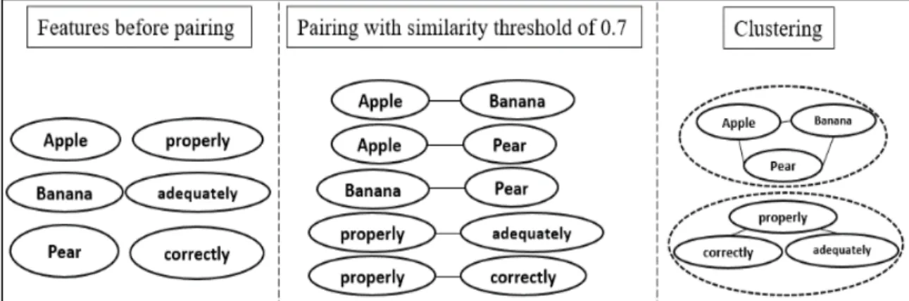
adjacent list with graph search algorithm (Breadth first search). Each connected component forms one cluster. One example of constructing clusters is shown in Fig. 2. The features before pairing are listed on the left of the graph. After pairing with the similarity threshold of 0.7, the pairs are shown in the middle of the graph. After running the clustering process, the “Apple - Banana” pair, “Apple - Pear” pair and “Banana - Pear” are clustered into “Apple, Banana, Pear”. So as “properly, adequately, correctly” cluster. Note that although these two clusters both contain three features, the similarities of these features in their cluster are not the same. For “Apple, Banana, Pear” cluster, since all three features have similarities higher than 0.7, the cluster is built as a complete graph. On the other hand, in “properly, adequately, correctly” cluster, only “properly- adequately” and “properly-correctly” have the similarity above 0.7 while “adequately” and “correctly” have similarity only about 0.5. Therefore, this cluster is formed as a tree and not all features have the similarity above the threshold. Thus, we call our clustering strategy as loose clustering. The benefit of using this loose clustering technique is that we can control the level of similarity of a cluster by changing the similarity threshold used in the pairing as well as the maximum allowed cluster size in clustering. Meanwhile, this type of clustering may cover more features at certain similarity threshold compared with other classic clustering techniques. The details of the effect of this type of cluster will be illustrated in the following section.
Fig. 2. An example process of constructing clusters from features.
v. Feature Reduction
Once the clusters are formed, features are reduced by replacing all the features in the cluster with a new feature, whose weight is the sum of the weight of all features in that cluster. This way of feature reduction is driven by the idea that there is no need to keep all semantically similar features separate. Instead, those similar features can be reduced into one new feature and this new feature carries the weight that contains all weights of that semantics. For example, originally, the feature “Apple”, “Banana” and “Pear” have the weight of 0.3 each and after the feature reduction, the individual feature of “Apple”, “Banana” and “Pear” are replaced with one feature of “Apple-Banana-Pear” whose weight is 0.9. Therefore, the total feature size is reduced by 2. The pseudo code of the feature reduction is described in Table 2.
vi. Classification and Comparison
The effect of our feature reduction method is evaluated using Multinomial Naïve Bayes classifier (NB), SVM classifier with linear kernel, K-Nearest-Neighbor (KNN), and Random Forest (RF) on all four datasets. The python implementation of these
our method is compared with the baseline to evaluate the effect of our method.
Meanwhile, the effect of applying our method after other feature reduction techniques, e.g. CS and MI, is also demonstrated with a variety number of selected feature size using 20-newsgroups dataset and R52 of Reuters-21578 dataset.
Table. 2. Pseudo code of feature reduction
Def createAdjList(pairs): adjList = {} For each pair:
If item1 or item2 in pair is in adjList: adjList(item1) add item2 in pair or
adjList(item2) add item1 in pair else: adjList(item1) = item2 or adjList(item2) = item1 return adjList Def buildCluster(adjList): clusters= [] visited = set() for key in adjList:
currCluster= [] queue.add(key)
while queue is not empty: vertex = queue.pop if vertex not in visited: visited.add(vertex) currCluster.add(vertex) queue.add(adjList[key]) if currCluster is not empty:
clusters.add(currCluster) return clusters
Def featureReduction(pairs, vector_matrix): adjList = createAdjList(pairs) clusters = buildCluster(adjList) for each cluster in clusters:
new_feature_col =
sum of vector_matrix with col_index in cluster vector_matrix.add(new_feature_col) vector_matrix.remove(col_index in cluster) return vector_matrix
IV. RESULTS i. Vectorization
After the vectorization, all samples in the four datasets are converted into vectors whose size are shown in Table 3. Although this size of the feature in 20-newsgroups, RCV1-v2 and R52 of Reuters-21578 seems large, recall that one of the goals of our study is to evaluate the effect of feature reduction, therefore, this feature set will be first used without other feature reduction techniques. Then for further investigation, we will demonstrate applying other feature reduction techniques and our method together for the feature reduction.
Table. 3. Training, testing and feature sizes of four datasets
Dataset Training size Testing size Feature size
20-newsgroups 11314 7532 101631
RCV1-v2 20000 392138 47236
R52 of Reuters 5754 2254 20354
ii. Paring
Our results of some similar pairs of words are shown in terms of different similarity ranges in Table 4.
Table. 4. Sample pairs of different similarities derived from Word2Vec
Similarity Pairs Percentage a
[0.9, 1.0) (East, west), (four, six), (forbids,
prohibits)… 0.016% [0.8, 0.9)
(electron, electrons), (electrons, photons), (embarrassing, embarassing), (enable, enabling) …
0.16%
[0.7, 0.8)
(entire, whole), (enzymes, protein), (epistemological, ontological), (hmm, hmmm), (erste, mogelijk), (increases,
decreases)…
0.78%
[0.6, 0.7) (entrepreneurs, startups), (oan, twa) 5.9%
[0.5, 0.6) (mjs, rw), (lori, Johnson), (increases,
increased)… 93%
a.The percentage is calculated from the number of the pairs in each similarity threshold range versus the
total number pairs above 0.5 similarity threshold.
It is noted that when the similarity is above 0.9, only the semantically similar words are paired. However, those pairs only make 0.016% of all the pairs. When similarity goes down to [0.8, 0.9], some pairs with the same stem (enable, enabling) or with very short edit distance or one letter misspelled (embarrassing, embarassing) also appear. On [0.7, 0.8) similarity category, some interjection pairs (hmm, hmmm) begin to appear and some foreign-language pairs also show up (erste, mogelij). On the range of
comes to [0.5, 0.6), more name pairs and meaningless phrases show up which making up 93% of all pairs. Another interesting observation is that a few antonyms are also paired (increases, decreases). Moreover, this antonym pair shows a similarity even higher than the synonym pair (increases, increased). The above observations indicate that the
similarity in Word2Vec not only reveals semantics but also shows clues in the relation of stemming, edit distance, interjection, multi-language, names, antonyms etc. Therefore, it is of great importance to carefully choose the similarity threshold before the feature reduction and more details of such relations in Word2Vec can be referred in [7].
iii. Clustering
The cluster sizes distributions of all four datasets are similar. Since
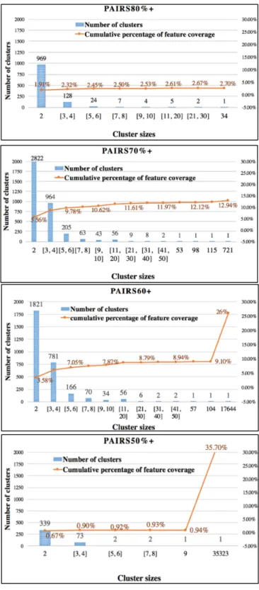
20-newspaper dataset contains the largest number of features sizes, the result of clustering on 20-newsgroups dataset is shown as an example in Fig.3. Pairs of 4 similarity thresholds of 0.8, 0.7, 0.6 and 0.5 are used, which are represented by PAIRS80%+, PAIRS70%+, PAIRS60%+ and PAIRS50%+ respectively. Two important factors are plotted in the figure to reveal the effect of the clustering: cluster size distribution and cumulative percentage of features covered in clustering. Cluster size distribution indicates the number of clusters with different cluster size range while the cumulative percentage of features indicates the potential extent of the feature reduction by applying our method. With the higher percentage of covered features, greater extent of feature reduction can be achieved. Additionally, with clusters covering the higher percentage of features, more effect of our methods can be reflected in the final results.
Fig. 3. Cluster size distribution with four similarity thresholds of 20-newsgroup dataset. Note that x-axis indicates the range of the cluster size; left y-axis indicates the number of
As suggested in Table 4, the pairs with the similarity threshold of 0.8 and above, which are in PAIRS80%+, have the strongest semantic connections. However, as shown in Fig. 3-PAIRS80%+, these pairs only cover up to 2.7% of the entire feature set. When the similarity threshold reduced to 0.7, which is shown in Fig. 3- PAIRS70%+, more numbers of small-size clusters (2,4, and 6) appears and around 10% of the features are covered. However, in PAIRS60%+, due to the relatively low similarity threshold, pairs with less semantic similarity are also included, which leads to a large chunk of cluster of 17644 features that takes over around 17% of the features with the smaller number of the small-size clusters. In Fig. 3- PAIRS50%+, the small size clusters continue to decrease while a gigantic cluster of size 35323 shows up which covers around 35% of the entire feature set. This large size of the cluster can show negative effect during clustering which will be discussed in the following paragraph.
iv. Feature Reduction and Classification
As PAIRS60%+, PAIRS70%+ and PAIRS80%+ show significant different cluster distributions in Fig. 3, the clusters constructed with these 3 similarity thresholds are used to investigate the effect of the cluster size and feature reduction on the
classification accuracy. As an example, the classification result of NB and SVM classifier on 20-newspaper is plotted as a function of the maximum allowed cluster size (MACS) in Fig. 4.
Fig. 4. F-score of PAIRS80%+, PAIRS70%+ and PAIRS60%+ in y-axis versus different MACSs in x-axis in 20-newspaper dataset. Baseline shows the F-Score
First, it is shown that the effect of PAIRS80%+ is relatively little by using either NB or SVM. In NB, the F-Score is increased by only 0.2% and in SVM, it is only up to 0.1%. This may due to the low feature coverage of PAIRS80%+. Even when MACS is set to ∞, the cumulative percentage of feature coverage is still 2.7%, which is indicated in Fig. 3.
By decreasing similarity threshold to PAIRS70%+, more features are covered and more effect on F-score is shown in the figure. First, higher F-scores are achieved for both NB and SVM in most cases of MACS compared with PAIRS80%+ and the baseline. This is because by increasing the feature coverage, more features with similar meanings are clustered which provides a better prediction rate. However, by continually lowering the similarity to PAIRS60%+, some side effects also appear. In NB, although
PAIRS60%+ outperforms in most of the MACSs, it also has a lower result than
PAIRS70%+ when MACS is 4. In SVM, PAIRS60%+ provides the lower F-scores than PAIRS70%+ in all MACSs. This result indicates the effect of semantic similarity derived from Word2Vec on the classification accuracy. As indicated in Table. 4, by decreasing the similarity thresholds, more pairs with less similarity are included in the cluster. Some words, that are not semantically similar, can also be paired and clustered, which explains the above results in our graph.
Meanwhile, the feature coverage can be also increased by increasing MACS, which results in a more significant influence on the classification accuracy. Especially in PAIRS70%+ and PAIRS60%+, most significant effects are observed. In Fig. 4, by increasing the MACS, the F-scores of both classifiers increase to a maximum value and
then drop. The highest increase in NB of around 0.4% is achieved in PAIRS60%+ with the MACS of 60 while in SVM, around 0.7% increase in PAIRS70%+ with the MACS of 9. These results correspond to the effect of the size of clusters. For one hand, when the MACS is low, only clusters with a small number of words are applied by our method. Recall that our features are only loosely clustered, which does not guarantee all features in the cluster are mutually semantically similar. With smaller size of the clusters, it is less likely for the cluster to contain pairs with semantic similarity less than the threshold. Especially, when MACS is 2, all pairs in the cluster have similarities above the threshold. Therefore, clustering plays a positive role in the prediction and better F-score is expected. However, with the MACS increases, more large-size clusters are also in effect. Large-size clusters are more likely to be mis-clustered. As we discussed above, our loose cluster is formed from the connected component other than the complete graph. With large-size connected component, there should be a large number of features that has the similarity less than the threshold, which may also be contained in the same cluster, leading to the poorer F-score. Especially when MACS is ∞, a dramatic drop is seen in F-score in both NB and SVM. In the case of PAIRS60%+, the F-score is even lower than the baseline in either NB or SVM with its largest cluster size of 17644. Therefore, it is seen that there is an optimal MACS in the cases of PAIRS70%+ and PAIRS60%+.
Finally, there is also a slight difference in F-score between NB and SVM. In theory, NB is the probability based classifier with high efficiency while SVM is more sophisticated and generally with higher accuracy if there are sufficient training samples
[15]. Thus, in our method, SVM provides higher F-score in all three similarity thresholds and MACSs.
Fig. 5 shows the percentage of the feature reduction as a function of F-score in both NB and SVM. First, since PAIRS80%+ only affected a little number of features (see Fig. 3), its influence on F-Score and feature reduction is also very limited. However, in the case of PAIRS70%+ and PAIRS60%+, the similar result in Fig. 4 is also observed in Fig. 5. First, F-score in NB is increased with feature reduction in PAIRS60%+ up to around 6%. However, no such trend is observed in PAIRS70%+. Then, F-score in SVM is increased with feature reduction in PAIRS70%+ up to 6.7% while a poor trend is seen in PAIRS60%+. To conclude, by using our method, we achieved a 6% feature reduction with F-Score increase by 0.4% in NB and a 7% feature reduction with 0.7% increase of F-Score in SVM.
Fig. 5. Percentage of feature reduction in x-axis versus F-Score with Naïve Bayes classifier and SVM classifier in y-axis in 20-newspaper dataset.
The complete classification results of all four classifiers on the four datasets are shown in Table 5.
Firstly, SVM provides the highest accuracy among all classifiers and datasets. The benefit of SVM is its ability to maximize margin for the decision boundary when the sample size is sufficient. Moreover, due to the characteristics of different datasets, the highest improvement of the classifier is achieved with different similarity thresholds and MACSs. The improvement of NB using our method is shown only in 20-newsgroups. Nevertheless, in other three datasets, there is no improvement of our methods with NB. As for KNN, the performance is highly depending on the dataset. In 20-newsgroups, since the feature size is large, the accuracy of KNN is extremely low, which may due to
the lack of the normalization. In RCV1-v2, it doesn’t even successfully accomplish the classification as its time complexity of KNN is relatively higher than other classifiers. However, in other two smaller-size datasets, by varying the factor K, the highest
improvement of our methods is shown with KNN compared with other classifiers, which is about 2-3 percentage of increase of classification accuracy. The reason for the largest improvement stems from the distance measure in KNN. As KNN uses Euclidean distance for measuring the distance to the neighbors, which is sensitive to the weight of the vector. Our method provides a way to improve the weight of the feature, thus improving the results of KNN most significantly. In RF, no significant effect is revealed in RF either by varying similarity thresholds or MACSs in our methods. In our study, the classification accuracy of RF is only effected by varying the estimator n. The reason may due to the random state of this classifier and the large variance of results covers the effects of our method.
The percentage of feature reduction when the highest F-score is achieved is also listed in the table and it is shown that the typical feature reduction is around 4 – 10% in terms of different datasets and classifiers. Thus, our method shows the improvement in the classification with different types of the classifiers and with the different types of the datasets including the one with the large feature size (20-newsgroups), the one with the large sample size (RCV1-v2), the one with the imbalanced categories (R52 of Reuters-21578), and the one with the specific domain (WebKB).
Additionally, our method can also as a supplemental step after other feature reduction techniques. Unlike the other techniques[13][14] with Word2Vec that are
designed to compete with classic feature reduction techniques, our method aims to improve the feature reduction rate and classification accuracy by acting as a succeeding step after the classic feature reduction. 20-newsgroups and R52 of Reuters-21578 datasets are used since the feature size of these two datasets are suitable for the feature reduction. Meanwhile, SVM is used as the measurement of the effect of feature reduction. Note that the similarity threshold is 70% and MACS is 9 for 20-newsgroups and the similarity threshold is 60% and MACS is 5 for R52 of Reuters-21578 for best results.
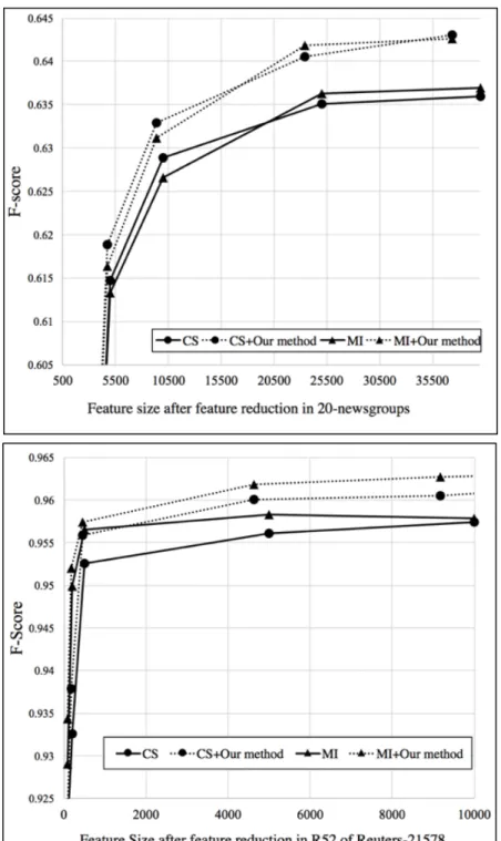
The result of our method with two classic feature reduction technique, CS, and MI, is shown in Fig. 6. As is shown in the graph, in both datasets, our method can
provide the improved F-scores with additional feature reduction at each feature size level. In 20-newsgourps dataset, the merit of our method is significant. For example, the F-score of CS plus our method at the feature size of around 10000 is comparable with the F-score of CS alone at the feature size of around 20000. In addition, the F-score of CS with our method with only around 25000 features has already outperformed the F-score of calculated with all 101631 features.
However, also note that the effect of our method is more significant when the feature size increases in R52 of Reuters-21578 dataset. The reason may due to the fact that only the words that can be found in Word2Vec model can be used to get its word embedding vector and make the similarity calculation. Thus, with more features involved, we may have higher chance to cluster the similar pairs and make our method effective.
Fig. 6. Feature size is shown in x-axis after feature reduction in two datasets versus F-Score shown in y-axis calculated using SVM classifier.
Table. 5. Classification result of four datasets 20-newsgroups PAIRS60%+ SVM NB KNN (k=3) KNN (k=5) KNN (k=8) RF (n=10) RF (n=30) Percentage of Feature reduction Baseline 63.80% 63.00% 16.06% 16.61% 17.27% 41.82% 52.11% - MACS=2 63.97% 63.15% - - - 41.69% 53.60% 1.79% MACS=3 64.13% 63.24% - - - 43.02% 52.30% 2.76% MACS=4 64.05% 63.21% - - - 41.90% 51.00% 3.61% MACS=5 63.94% 63.25% - - - 42.11% 52.92% 4.03% MACS=9 63.95% 63.30% - - - 41.10% 53.32% 4.92% MACS=60 64.09% 63.45% - - - 42.32% 52.90% 6.11% No size limit 63.00% 62.29% - - - 42.09% 51.99% 6.20% PAIRS70%+ MACS=2 64.04% 63.00% - - - 42.73% 52.52% 2.78% MACS=3 64.32% 63.07% - - - 41.59% 53.23% 4.06% MACS=4 64.34% 63.31% - - - 42.22% 52.55% 4.98% MACS=5 64.45% 63.24% - - - 43.22% 52.79% 5.51% MACS=9 64.53% 63.05% - - - 42.07% 53.01% 6.49% MACS=60 64.50% 63.19% - - - 43.15% 52.88% 7.91% No size limit 64.15% 63.03% - - - 42.07% 52.66% 8.80% PAIRS80%+ MACS=2 63.88% 63.13% - - - 1.0% MACS=3 63.90% 63.14% - - - 1.1% MACS=4 63.75% 63.13% - - - 1.2% MACS=5 63.73% 63.18% - - - 1.30% MACS=9 63.78% 63.20% - - - 1.60% No size limit 63.78% 63.20% - - - 1.60%
RCV1-v2 PAIRS60%+ SVM NB KNN (k=3) KNN (k=5) KNN (k=8) RF (n=10) RF (n=30) Percentage of Feature reduction Baseline 78.97% 77.85% - - - 72.73% - MACS=3 79.04% 77.76% - - - 73.28% - 2.50% MACS=5 79.17% 77.72% - - - 72.67% - 3.20% MACS=7 79.43% 77.63% - - - 72.85% - 3.46% MACS=9 79.41% 77.56% - - - 73.00% - 3.71% MACS=20 79.28% 77.52% - - - 72.18% - 4.41% MACS=30 78.50% 77.35% - - - 73.09% - 4.87% MACS=60 78.51% 77.38% - - - 72.87% - 5.23% PAIRS70%+ MACS=3 79.06% 77.87% - - - 73.18% - 1.89% MACS=5 79.19% 77.82% - - - 72.36% - 2.10% MACS=7 79.17% 77.82% - - - 73.87% - 2.18% MACS=9 79.31% 77.82% - - - 73.00% - 2.24% MACS=20 79.24% 77.75% - - - 72.80% - 2.49%
R52 of Reuters-21578 PAIRS60%+ SVM NB KNN (k=3) KNN (k=5) KNN (k=8) RF (n=10) RF (n=30) Percentage of Feature reduction Baseline 95.92% 95.39% 85.63% 86.42% 86.78% 87.93% 89.88% - MACS=3 96.27% 95.25% 86.07% 87.49% 87.49% 88.73% 89.83% 6.24% MACS=5 96.41% 94.90% 86.51% 87.67% 87.80% 88.29% 90.51% 9.28% MACS=7 96.27% 95.12% 86.87% 87.71% 88.07% 87.27% 89.93% 10.96% MACS=9 96.18% 95.08% 86.69% 87.76% 88.02% 88.38% 90.37% 12.04% MACS=20 95.92% 94.81% 87.00% 88.29% 88.29% 88.15% 90.73% 14.69% MACS=30 96.23% 94.63% 87.44% 87.89% 88.60% 87.31% 90.64% 15.64% MACS=60 96.18% 94.59% 87.84% 88.07% 88.38% 86.91% 90.46% 16.88% PAIRS70%+ MACS=3 95.92% 95.16% 86.87% 87.58% 87.84% 88.64% 89.62% 7.95% MACS=5 96.05% 95.21% 87.22% 87.89% 88.02% 88.55% 90.99% 10.40% MACS=7 96.18% 94.94% 87.27% 87.89% 88.07% 87.89% 89.62% 11.44% MACS=9 96.18% 95.03% 87.58% 88.24% 88.69% 89.53% 90.28% 12.22% MACS=20 96.14% 94.72% 87.67% 88.11% 88.33% 87.53% 90.59% 13.53% MACS=30 96.36% 94.72% 87.89% 87.98% 88.38% 87.53% 91.22% 13.74% MACS=60 96.23% 94.72% 87.84% 87.98% 88.20% 87.80% 90.28% 13.88%
WebKB PAIRS60%+ SVM NB KNN k=3 KNN k=5 KNN k=8 RF n=10 RF n=30 Percentage of Feature reduction Baseline 90.26% 82.45% 66.55% 66.53% 65.05% 81.40% 83.30% - MACS=3 90.47% 81.88% 67.13% 67.51% 66.48% 79.53% - 3.53% MACS=5 90.47% 81.88% 66.85% 67.45% 67.18% 79.63% - 4.65% MACS=7 91.17% 81.52% 67.20% 67.10% 67.56% 81.69% - 5.59% MACS=9 89.97% 81.30% 67.09% 67.24% 67.51% 80.85% - 5.79% MACS=20 90.11% 81.16% 67.16% 67.24% 67.51% 81.45% - 6.33% MACS=60 90.11% 81.16% 67.16% 67.24% 67.51% 80.23% - 6.33% No size limit 89.33% 81.02% 65.74% 64.25% 61.75% 80.68% - 17.66% PAIRS70%+ MACS=3 90.69% 82.02% 66.71% 66.88% 65.91% 80.71% - 1.67% MACS=5 90.62% 81.81% 66.74% 66.99% 66.24% 81.42% - 2.02% MACS=7 90.62% 81.81% 66.74% 66.99% 66.24% 81.71% - 2.10% MACS=9 90.69% 81.81% 66.74% 66.99% 66.24% 81.21% - 2.20% MACS=20 90.69% 81.81% 66.74% 66.95% 66.46% 82.37% - 2.88% MACS=30 90.69% 81.81% 66.69% 66.78% 66.16% 82.36% - 3.61% MACS=60 90.69% 81.81% 66.69% 66.78% 66.16% 80.41% - 3.61% No size limit 90.90% 81.95% 66.65% 67.30% 66.14% 83.68% - 4.51%
V. DISCUSSION
Recall that some improvements are achieved in our method in terms of the feature reduction, classification accuracy and working with other classic feature reduction techniques, however, compared with the baseline, the absolute accuracy improvements of our method in our classifiers are still not very significant. Serval factors may contribute to this result. Firstly, the intrinsic mechanism of the similarity measure in Word2Vec is not well understood at this point. The similarity threshold alone may not sufficient to identify the semantically similar pairs. One solution in our method is to raise the threshold as in PAIRS80%+. However, due to the low coverage of features, although only a few mis-clustering, the improvement is really limited. Therefore, we have to lower the similarity threshold down to PAIRS60%+ to allow more pairs involved. But this can bring another problem. As we discussed above, when the similarity threshold is
decreased, some other pairs with less semantic similarity, including interjection, person’s name etc., are also included in the cluster. Some originally semantically similar words (increases, increased) can even have a similarity 10% lower than the pairs that have the opposite meaning (increases, decreased). Therefore, the optimal result in our method is the combination of the cost of the increased mis-clustering ratio and the product of the higher percentage of feature coverage, which finally achieved a maximum F-score at certain MACS. After all, the final solution of this problem requires a better understanding of the intrinsic mechanism of Word2Vec so as to better identify the pairs with high semantic similarity.
Secondly, the dataset itself also obscures the performance of our method. As the 20-newsgroups dataset is very popular among the NLP field, it contains some categories that are very distinct from each other as well as some that are really closely related [17]. Therefore, this characteristic makes the dataset a good candidate to measure the
performance of a classifier in terms of different categories. Thus, in order to better unveil the effect of our method, we choose the 4, 6, 8, 10 and 12 most distinct categories of the entire dataset as our subset. Since PAIRS60%+ with MACS of 60 is performed best in NB and PAIRS70%+ with MACS of 9 is the best in SVM, those two clustering strategies are used. Move over, we further remove the documents which have no features that are clustered (which means no feature has been removed or added) to better show the effect of our method.
The number of documents in each category of the dataset before and after the adjustment is described in Table 6. Firstly, it is a balanced dataset since the number of articles for each category is relatively the same. Secondly, after removing the non-affected articles, 5-10% articles are removed in each category and around 90% of the entire dataset remain in our following investigation as shown in two columns of “Adjusted” in Table 6.
Meanwhile, while some categories are highly distinct (e.g. index 4, 8, 12 and 18), among all these 20 categories, some are closely related (e. g. 2 vs. 4 and 9 vs. 10). Therefore, subsets of 4, 6, 8, 10, 12 and 20 categories are selected and used to better evaluate the effect of our method.
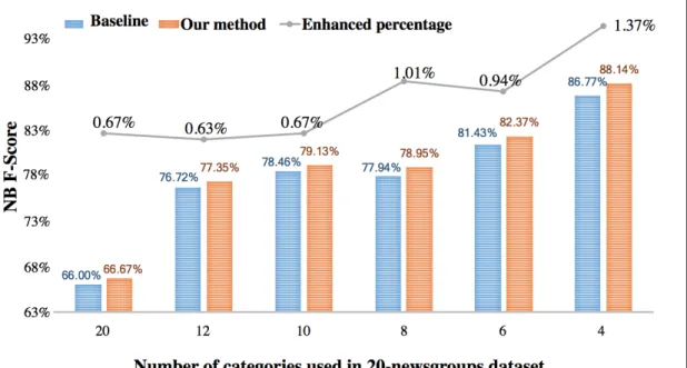
The results with the chosen subset are shown in Fig. 7. The plot shows the F-score of the baseline and our method among 6 different sizes of categories. The
improvement of our method versus the baseline is plotted as gray lines in the figure. It is shown that in “20 categories”, by only removing the unchanged documents, both baseline and our method present a better result than our result with the entire dataset (around 3% increase in NB and around 2% increase in SVM). This is largely due to the removal of extremely short documents which carries far fewer words. In addition, by removing the unchanged documents, the improvement of our method increased from 0.4% to 0.7% (NB) and 0.7% to 1.1% (SVM) respectively in “20 categories”. By continually removing some obscure categories, the improved percentage of our method continue to grow. At the point of “4 categories (4, 8, 12, 18)”, our method shows 1.4% improvement in NB and 2.0% improvement in SVM than the baseline, which indicates the effectiveness of our method.
In RCV1-v2, the improvement of our method is the least significant than other datasets. The reason may due to the low percentage of feature reduction, which means our Word2Vec model doesn’t have sufficient vocabulary to cluster features in RCV1-v2, which results in the less improvement in either feature reduction or classification
Table. 6. Number of samples in 20 Categories before and after Adjust in 20-newsgroups dataset
Cat# Name Total Adjusteda Adjustedb
0 alt.atheism 799 721 767 1 comp.graphics 973 894 929 2 comp.os.ms-windows.misc 985 883 932 3 comp.sys.ibm.pc.hardware 982 912 948 4 comp.sys.mac.hardware 963 863 899 5 comp.windows.x 988 915 955 6 misc.forsale 975 900 930 7 rec.autos 990 856 903 8 rec.motorcycles 996 870 925 9 rec.sport.baseball 994 863 909 10 rec.sport.hockey 999 904 955 11 sci.crypt 991 900 940 12 sci.electronics 984 904 931 13 sci.med 990 911 944 14 sci.space 987 913 938 15 soc.religion.christian 997 941 966 16 talk.politics.guns 910 838 871 17 talk.politics.mideast 940 862 898 18 talk.politics.misc 775 712 739 19 talk.religion.misc 628 552 586
a. lists the affected articles after clustering with PAIRS60%+ and MACS of 60. b. lists the articles with PAIRS70%+ and MACS of 10.
Fig. 7. Comparison of the F-Scores between the baseline and our method using the subsets of 20-newsgroups dataset with decreasing number of categories. E.g. 12 means 12 categories in 20-newsgroups dataset are used as a subset. Note that the y -axis is the F-score after classification using NB or SVM; the x-axis shows the number of categories in the descending order. The enhanced percentage of our method is shown in a gray line.
In R52 of Reuters-21578 dataset, as its categories are highly imbalanced, the majority of the sample sizes are in the categories that can be classified with fairly high accuracy with both baseline and our method. Therefore, to better reveal the effect of our method, by applying the similar strategy as in 20-newsgroups, we select 6 categories ('crude', 'trade', 'interest', 'ship', 'money-supply', 'coffee') among the 10 and the result is shown in Table 7. As is seen in the table, all four classifiers have the improved results. Note that even for NB, which does not show any improvement in the full R52 of Reuters-21578 dataset, also shows an improvement of 1.1%. As for RF, the effect of our method is significant to overcome the variance of its results and show an improvement of around 4%.
Table. 7. Improvement of classification accuracy in R52 of Reuters-21578 dataset with different classifiers
Baseline Our method Enhanced percentage
SVM 92.28% 93.93% 1.6% NB 90.9% 92.01% 1.1% KNN (k=3) 78.78% 82.1% 3.4% KNN (k=5) 78.86% 81.27% 2.4% KNN (k=8) 77.42% 79.34% 1.9% RF (n=10) 81.27% 85.67% ~4%
As for WebKB, its sample size is the smallest among the four datasets and the category domain is very specific to the college system. Therefore, since our current Word2Vec model is not sufficiently refined to the college system, a more specific model which is trained with abundant domain knowledge will be helpful to further improve its accuracy.
VI. CONCLUSION AND FUTURE WORK
Feature reduction is successfully improved using our method by utilizing Word2Vec with increased classification accuracy. We utilize four different types of classifiers and two types of classic feature reduction techniques on four different datasets to evaluate the effect of our method. The result shows that around 4-10% feature
reduction is achieved with up to 1-4% improvement in terms of different datasets and classifiers. Different classifiers perform differently in our study. SVM achieves the highest classification accuracy in all four datasets; NB is effective in 20-newsgroups dataset; KNN shows the highest improvement when comparing with our method with the baseline in R52 of Reuters-21578 dataset and WebKB dataset; In RF, no significant improvement is shown in most cases of our method since the variance of its prediction result covers the improvement of our method but a significant improvement is shown when a subset of R52 of Reuters-21578 is used. Meanwhile, we also show that our method can successfully improve feature reduction and classification accuracy after CS and MI.
The future work of this study would continue focusing on refining the loose clustering technique, which would allow us to better control the ratio of features that have similarity lower than the threshold. Meanwhile, when the categories are closely related or when encountering a specialized dataset whose vocabulary is not well covered in our Word2Vec model, the effect of our method is not well effective. To solve this problem, instead of using some generally trained corpus, a refined text corpus that is closely
we may use that specific model to calculate the word similarities so as to better classify those categories.
REFERENCES
[1] B. Li, “Importance weighted feature selection strategy for text classification,” 2016 International Conference on Asian Language Processing (IALP), Tainan, 2016, pp. 344-347.
[2] Y. Xu and L. Chen, “Term-frequency Based Feature Selection Methods for Text Categorization,” 2010 Fourth International Conference on Genetic and Evolutionary Computing, Shenzhen, 2010, pp. 280-283.
[3] A. L. Blum, and P. Langley, “Selection of relevant features and examples in machine learning”, Artificial Intelligence, vol. 97, Issue 1, pp 245-271, 1997
[4] G. Xu, C. Wang, L. Wang, Y. Zhou, W. Li, H. Xu, and Q. Huang, “Semantic classification method for network Tibetan corpus,” Cluster Comput vol. 20, pp. 155– 165, March 2017.
[5] S. S. Desai and J. A. Laxminarayana, “WordNet and Semantic similarity based approach for document clustering,” International Conference on Computation System and Information Technology for Sustainable Solutions (CSITSS), Bangalore, 2016, pp. 312-317.
[6] T. Mikolov, I. Sutskever, K. Chen, G. Corrado, and J. Dean, “Distributed Representations of Words and Phrases and their Compositionality,” Advances in Neural Information Processing Systems 26, pp. 3111–3119, 2013.
[7] Y. Zhang, A. Jatowt and K. Tanaka, “Towards understanding word embeddings: Automatically explaining similarity of terms,” 2016 IEEE International Conference on Big Data (Big Data), Washington, DC, 2016, pp. 823-832.
[8] S. Moran, R. Mccreadie, C. Macdonald, and I. Ounis, “Enhancing First Story Detection using Word Embeddings,” SIGIR 2016, Pisa, Italy, pp. 821-824, 17-21 July 2016. [9] S. Jiang, J. Lewris, M. Voltmer, and H. Wang, “Integrating rich document
representations for text classification.” Systems and Information Engineering Design Symposium (SIEDS), 2016 IEEE, pp. 303-308, 2016.
[10] A. K. Vijayakumar, R. Vedantam, and D. Parikh, “Sound-Word2Vec: Learning Word Representations Grounded in Sounds,” arXiv preprint arXiv:1703.01720, 2017. [11] D. Duong, E. Eskin, and J. Li, “A novel Word2vec based tool to estimate semantic
similarity of genes by using Gene Ontology terms,” Cold Spring Harbor Labs Journals, bioRxiv, pp. 103648, Jan 2017.
[12] J. Lilleberg, Y. Zhu and Y. Zhang, “Support vector machines and Word2vec for text classification with semantic features,” 2015 IEEE 14th International Conference on Cognitive Informatics & Cognitive Computing (ICCI*CC), Beijing, 2015, pp. 136-140.
[13] M. Feng, and G. Wu, “A Distributed Chinese Naive Bayes Classifier Based on Word Embedding,” International Conference on Machinery, Materials and Computing Technology (ICMMCT 2016), pp 1121-1127, 2016.
[14] W. Rui, J. Liu, and Y. Jia, “Unsupervised feature selection for text classification via word embedding,” Big Data Analysis (ICBDA), 2016 IEEE International Conference on. IEEE, 2016.
[15] R. Caruana and A.Niculescu-Mizil. “An empirical comparison of supervised learning algorithms.” Proceedings of the 23rd international conference on Machine learning (ICML '06). ACM, New York, NY, USA, 161-168. 2006
[16] Some Text Datasets. Available at
http://www.cs.umb.edu/~smimarog/textmining/datasets/, 2007.
[17] Home Page for 20 Newsgroups Data Set. Available at
http://qwone.com/~jason/20Newsgroups/, 2008.
[18] D. Lewis.; Y. Yang; T. Rose; and F. Li, RCV1: A New Benchmark Collection for Text Categorization Research. Journal of Machine Learning Research, 5:361-397, 2004.