Variational Bayesian dropout: pitfalls and fixes

(1)

Jiri Hron1 Alexander G. de G. Matthews1 Zoubin Ghahramani1 2

Abstract

Dropout, a stochastic regularisation technique for training of neural networks, has recently been reinterpreted as a specific type of approximate inference algorithm for Bayesian neural networks. The main contribution of the reinterpretation is in providing a theoretical framework useful for analysing and extending the algorithm. We show that the proposed framework suffers from several issues; from undefined or pathological behaviour of the true posterior related to use of improper priors, to an ill-defined variational objective due to singularity of the approximating distribution relative to the true posterior. Our analysis of the improper log uniform prior used in variational Gaussian dropout suggests the pathologies are generally irredeemable, and that the algorithm still works only because the variational formu-lation annuls some of the pathologies. To ad-dress the singularity issue, we proffer Quasi-KL (QKL) divergence, a new approximate inference objective for approximation of high-dimensional distributions. We show that motivations for varia-tional Bernoulli dropout based on discretisation and noise have QKL as a limit. Properties of QKL are studied both theoretically and on a sim-ple practical examsim-ple which shows that the QKL-optimal approximation of a full rank Gaussian with a degenerate one naturally leads to the Prin-cipal Component Analysis solution.

1. Introduction

Srivastava et al.(2014) proposed dropout as a cheap way of preventing Neural Networks (NN) from overfitting. This work was rather impactful and sparked large inter-est in studying and extending the algorithm. One strand of this research lead to reinterpretation of dropout as a form of

1

Department of Engineering, University of Cambridge, Cam-bridge, United Kingdom2Uber AI Labs, San Francisco, California, USA. Correspondence to: Jiri Hron<[email protected]>.

Proceedings of the35th

approximate Bayesian variational inference (Kingma et al., 2015;Gal & Ghahramani,2016;Gal,2016).

There are two main reasons for attempting reinterpretation of an existing method: 1) providing a principled interpre-tation of the empirical behaviour; 2) extending the method based on the acquired insights. Variational Bayesian dropout has been arguably successful in meeting the latter criterion (Kingma et al.,2015;Gal,2016;Molchanov et al.,2017). This paper thus focuses on the former by studying the theo-retical soundness of variational Bayesian dropout and the im-plications for interpretation of the empirical results. The first main contribution of our work is identifica-tion of two main sources of issues in current variaidentifica-tional Bayesian dropout theory:

(a) use of improper or pathological prior distributions; (b) singularity of the approximate posterior distribution. As we describe in Section 3, the log uniform prior in-troduced in (Kingma et al.,2015) generally does not in-duce a proper posterior, and thus the reported sparsifi-cation (Molchanov et al.,2017) cannot be explained by the standard Bayesian and the related minimum descrip-tion length (MDL) arguments. In this sense, sparsificadescrip-tion via variational inference with log uniform prior falls into the same category of non-Bayesian approaches as, for exam-ple, Lasso (Tibshirani,1996). Specifically, the approximate uncertainty estimates do not have the usual interpretation, and the model may exhibit overfitting. Consequently, we study the objective from a non-Bayesian perspective, prov-ing that the optimised objective is impervious to some of the described pathologies due to the properties of the varia-tional formulation itself, which might explain why the algo-rithm can still provide good empirical results.1

Section4shows how mismatch between support of the ap-proximate and the true posterior renders application of the standard Variational Inference (VI) impossible by mak-ing the Kullback-Leibler (KL) divergence undefined. As the second main contribution, we address this issue by prov-ing that the remedies to this problem proposed in (Gal & Ghahramani,2016;Gal,2016) are special cases of a broader

1

An earlier version of this work was published in (Hron et al.,

(2)

class of limiting constructions leading to a unique objective which we name Quasi-KL (QKL) divergence.

Section5provides initial discussion of QKL’s properties, uses those to suggest an explanation for the empirically ob-served difficulty in tuning hyperparameters of the true model (e.g.Gal(2016, p. 119)), and demonstrates the potential of QKL on an illustrative example where we try to approxi-mate a full rank Gaussian distribution with a degenerate one using QKL, only to arrive at the well known Principal Component Analysis (PCA) algorithm.

2. Background

Assume we have a discriminative probabilistic model y|x,W ∼ P(y|x,W) where (x, y) is a single input-output pair, andW is the set of model parameters gen-erated from a prior distribution P(W). In Bayesian inference, we usually observe a set of data points (X,Y) = {(xn, yn)}Nn=1 and aim to infer the posterior

p(W |X,Y)∝p(W)Q

np(yn|xn,W),

2_{which can be} subsequently used to obtain the posterior predictive density p(Y0|X0,X,Y) = R

p(Y0|X0,W)p(W |X,Y)dW. Ifp(y|x,W)is a complicated function ofW like a neural network, both tasks often become computationally infeasi-ble and thus we need to turn to approximations.

Variational inference approximates the posterior distribution over a set of latent variablesW by maximising the evidence lower bound (ELBO),

L(q) = E

Q(W)[logp(Y |X,W)]−KL (Q(W)kP(W)),

with respect to (w.r.t.) an approximate posteriorQ(W). If Q(W)is parametrised byψand the ELBO is differentiable w.r.t.ψ, VI turns inference into optimisation. We can then approximate the density of posterior predictive distribution using q(Y0|X0,X,Y) = R

p(Y0|X0,W)q(W)dW, usually by Monte Carlo integration.

A particular discriminative probabilistic model is a Bayesian neural network (BNN). BNN differs from a standard NN by assuming a prior over the weightsW. One of the main advantages of BNNs over standard NNs is that the posterior predictive distribution can be used to quantify uncertainty when predicting on previously unseen data(X0,Y0). How-ever, there are at least two challenges in doing so:

1) difficulty of reasoning about choice of the priorP(W); 2) intractability of posterior inference.

For a subset of architectures and priors, Item1can be ad-dressed by studying limit behaviour of increasingly large

2

Throughout the paper,P(W)refers to the distribution and p(W)to its density function. Analogously for other distributions.

networks (see, for example, (Neal,1996;Matthews et al., 2018)); in other cases, sensibility of P(W) must be as-sessed individually. Item2necessitates approximate infer-ence – a particular type of approximation related to dropout, the topic of this paper, is described below.

Dropout (Srivastava et al.,2014) was originally proposed as a regularisation technique for NNs. The idea is to multiply inputs of a particular layer by a random noise variable which should prevent co-adaptation of individual neurons and thus provide more robust predictions. This is equivalent to multi-plying the rows of the subsequent weight matrix by the same random variable. The two proposed noise distributions were Bernoulli(p)and GaussianN(1, α).

Bernoulli and Gaussian dropout were later respectively rein-terpreted byGal & Ghahramani(2016) andKingma et al. (2015) as performing VI in a BNN. In both cases, the appro-ximate posterior is chosen to factorise either over rows or individual entries of the weight matrices. The prior usually factorises in the same way, mostly to simplify calculation ofKL (Q(W)kP(W)). It is the choice of the prior and its interaction with the approximating posterior family that is studied in the rest of this paper.

3. Improper and pathological posteriors

BothGal & Ghahramani(2016) andKingma et al.(2015) propose using a prior distribution factorised over individ-ual weights w ∈ W. While the former opts for a zero mean Gaussian distribution,Kingma et al.(2015) choose to construct a prior for whichKL (Q(W)kP(W))is indepen-dent of the mean parametersθof their approximate posterior q(w) =φθ,αθ2(w),w∈W, θ∈θ, whereφ_µ,σ2is the

den-sity function ofN(µ, σ2₎_{. The decision to pursue such}

independence is motivated by the desire to obtain an algo-rithm that has no weight shrinkage – that is to say one where Gaussian dropout is the sole regularisation method. Indeed, the authors show that the log uniform priorp(w) := C/|w| is the only one whereKL (Q(W)kP(W))has this mean parameter independence property. The log uniform prior is equivalent to a uniform prior onlog|w|. It is an improper prior (Kingma et al.,2015, p. 12) which means that there is noC∈Rfor whichp(w)is a valid probability density.

Improper priors can sometimes lead to proper posteriors (e.g. normal Jeffreys prior for Gaussian likelihood with unknown mean and variance parameters) ifCis treated as a positive finite constant and the usual formula for computation of posterior density is applied. We show this is generally not the case for the log uniform prior, and that any remedies in the form of proper priors that are in some sense close to the log uniform (such as uniform priors over floating point numbers) will lead to severely pathological inferences.

(3)

−δ δ r

Figure 1.Illustration of Proposition1. Blue is the prior, orange the likelihood, and green shows a particular neighbourhood ofw= 0where the likelihood is greater thanr >0(such neighbourhood exists by the continuity). Integral of the likelihood over(−δ, δ)

w.r.t.P(w)diverges because the likelihood can be lower bounded byr >0and the prior assigns infinite mass to this neighbourhood.

3.1. Pathologies of the log uniform prior

For any proper posterior density, the normaliser Z = R

RDp(Y |X,W)p(W)dW has to be finite (D denotes the total number of weights). We will now show that this requirement is generally not satisfied for the log uniform prior combined with commonly used likelihood functions. Proposition 1. Assume the log uniform prior is used and that there exists some w ∈ W such that the likelihood function atw= 0is continuous inwand non-zero. Then the posterior is improper.

All proofs can be found in the appendix. Notice that stan-dard architectures with activations like rectified linear or sigmoid, and Gaussian or Categorical likelihood satisfy the above assumptions, and thus the posterior distribution for non-degenerate datasets will generally be improper. See Figure1for a visualisation of this case.

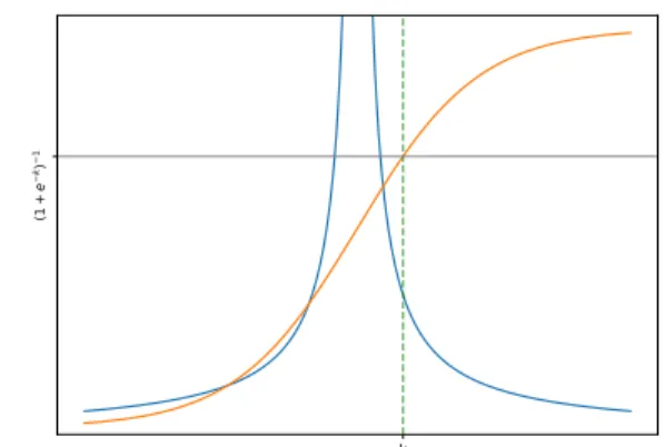
Furthermore, the pathologies are not limited to the region nearw= 0, but can also arise in the tails (Figure2). As an example, we will consider a single variable Bayesian logistic regression problemp(y|x, w) = 1/(1 + exp(−xw)), and again use the log uniform prior forw. For simplicity, assume that we have observed(x = 1, y = 1)and wish to infer the posterior distribution. To show that the right tail has infinite mass, we integrate over[k,∞), k >0,

k (1 + e − k) − 1

Figure 2.Visualisation of the infinite tail mass example. Blue is the prior, orange the sigmoid likelihood, and green shows the lower bound of the[k,∞)interval. The sigmoid function is greater than zero for anyk >0. The integral of the likelihood over[k,∞)w.r.t.

P(w)can thus again be lower bounded by a diverging integral.

(x=−1, y= 1). Because the sigmoid function is continu-ous and equal to1/2atw= 0, the posterior also has infinite mass around the origin, exemplifying both of the discussed degeneracies. The normalising constant is of course still infinite and thus the posterior is again improper.

The practical implication of these pathologies is that even tasks as simple as MAP estimation (Proposition1implies unbounded posterior density) or posterior mean estimation will fail as the target is undefined. In general, improper pos-teriors lead to undefined or incoherent inferences. The above shows that this is the case for the log uniform prior com-bined with BNNs and related models, making Bayesian inference, exact and approximate, ill-posed.

3.2. Pathologies of the truncated log uniform prior Neklyudov et al.(2017) proposed to swap the log uniform prior on(−∞,∞)for a distribution that is uniform on a suf-ficiently wide bounded interval in thelog|w|space (will be referred to asthe log spacefrom now on), i.e.p(log|w|) = 1/(b−a)_I[a,b](w), a < bwhereIAis the indicator

func-tion of the setA. This prior can be used in place of the log uniform if the induced posteriors in some sense converge to a well-defined limit for any dataset as[a, b]gets wider. If this is not the case, choice of[a, b]becomes a prior assump-tion and must be justified as such because different choices will lead to sometimes considerably different inferences. We now show that posteriors generally do not converge for the truncated log uniform prior and discuss some of the related pathologies of the induced exact posterior. To illustrate the considerable effect the choice of[a, b]might have, we return to the example of posterior inference in a logistic regression modelp(y|x, w) = 1/(1 + e−xw₎

(4)

−e−bn _−e−an_ean _ebn w ∝ 1 / | w |

Figure 3.A truncated log uniform prior transformed to the original space. Notice that the support gap around the origin narrows as an→ −∞, and the tail support expands asbn→ ∞which yields

the more pathological inferences the wider[an, bn]gets.

IIn(w) Cn/|w| where In = [−e

bn_,_−ean_] _∪ _[ean_,_ebn_] (i.e. the appropriate transformation of the closed interval [an, bn]fromthe log space– see Figure3). We exemplify

the sensitivity of the posterior distribution to the choice of the(In)n∈Nsequence by studying the limiting behaviour of the posterior mean and variance. Using the definition of

IIn(w)and symmetry, the normaliser of the posterior is, Zn= Z −ean −ebn 1 |w| 1 1 + e−wdw+ Z ebn ean 1 |w| 1 1 + e−wdw = Z ebn ean 1 |w| 1 + ew 1 + ewdw=bn−an.

Similar ideas can be used to derive the first two moments,

E Pn (w) = Rebn ean 1 1+e−wdw− R−ean −ebn 1 1+e−wdw bn−an =h(e

bn_{) +}_h(−ebn₎₋_h(ean₎₋_h(−ean₎ bn−an , (1) E Pn (w2) = Z ebn ean |w| bn−an 1 + ew 1 + ewdw= e2bn₋_e2an 2(bn−an) , (2) whereh(x) := log(1 + ex₎_{, and}_P

nstands forPn(w|x, y).

To understand sensitivity of the posterior mean to the choice of(In)n∈N, we now construct sequences which respectively lead to convergence of the mean to zero, an arbitrary positive constant, and infinity.3 To emphasise this is not specific to the posterior mean, we show that the variance might equally well be zero, infinite, or undefined.

To getlimn→∞EPn(w) = 0, notice that for a fixed bn, the second term in Equation (1) tends tolog(4)/∞ = 0.

3

It would be equally possible to get convergence to an arbitrary negative constant, and negative infinity if the observation was

(x=−1, y= 1).

Hence we can make the posterior mean converge to zero by making the first term also tend to zero; a way to achieve this is settingbn= log(log|an|), which tends to infinity as

an→ ∞. The limit of Equation (2) for the same sequence,

and thus the variance, tends to zero as well.

Forlimn→∞EPn(w) =c >0, we again focus on the first term in Equation (1) as the second term tends to zero for any increasing sequenceIn%R. Simple algebra shows that for

any diverging sequencebn→ ∞, takingan =bn−ebn/c

yields the desired result. The same sequence leads to infinite second moment and thus to infinite variance.

Finally, a choice which results in infinite mean and thus undefined variance is settingan =−bn, for which the mean

grows asebn_/b

n. We would like to point out that this

sym-metric growth ofanwithbnis of particular interest as it

corresponds to changing between different precisions of the float format representation on the computer as consid-ered inKingma et al.(2015, Appendix A).

3.3. Variational Gaussian dropout as penalised maximum likelihood

We have established that optimisation of the ELBO im-plied by a BNN with log uniform prior over its weights cannot generally be interpreted as a form of approximate Bayesian inference. Nevertheless, the reported empirical results suggest that the objective might possess reasonable properties. We thus investigate if and how the pathologies of the true posterior translate into the variational objective as used in (Kingma et al.,2015;Molchanov et al.,2017). Firstly, we derive a new expression forKL (Q(w)kP(w)), and for its derivative w.r.t. the variational parameters, which will help us with further analysis.

Proposition 2. Letq(w) =φµ,σ2(w), andp(w) = C/|w|.

Denoteu:=µ2_/(2σ2₎_{. Then,} KL (Q(w)kP(w)) =const.+1 2 log 2 + e−u ∞ X k=0 uk k!ψ(1/2 +k) (3) =const.−1 2 ∂M(a; 1/2;−u) ∂a _a₌₀ , (4)

whereψ(x)denotes the digamma function, andM(a;b;z)

the Kummer’s function of the first kind. We can obtain gradients w.r.t.µandσ2_using,

∇uKL (Q(w)kP(w)) =    1 u= 0 D+( √ u) √ u u >0 , (5)

and the chain rule; D+(x) is the Dawson integral.

(5)

Before proceeding, we note that Equation (5) is sufficient to implement first order gradient-based optimisation, and thus can be used to replace the approximations used in (Kingma et al.,2015;Molchanov et al.,2017). Note that numeri-cally accurate implementations of theD+(x)exist in many

programming languages (e.g. (Johnson,2012)).

In VI literature, the termKL (Q(w)kP(w))is often inter-preted as a regulariser, constrainingQ(w)from concentrat-ing at the maximum likelihood estimate which would be optimal w.r.t. the other termEQ(W)[logp(Y |X,W)]in

the ELBO. It is thus natural to ask what effect this term has on the variational parameters. Noticing that only the in-finite sum in Equation (3) depends on these parameters, and that the first summand is always equal toψ(1/2), we can focus on terms corresponding to k ≥ 1. Because ψ(1/2 +k)>0,∀k≥1, all summands are non-negative. Hence the penalty will be minimised ifµ2_/(2σ2_{) = 0}_{, i.e.}

whenµ = 0and/orσ2 _{→ ∞}_{; Corollary}₃_{is sufficient to}

establish that this minimum is unique.

Corollary 3. Under assumptions of Proposition 2,

KL (Q(w)kP(w))is strictly increasing foru∈[0,∞).

Sections3.1and3.2suggests the pathological behaviour is non-trivial to remove unless we replace the (truncated) log uniform prior.4 _{An alternative route is to interpret} optimi-sation of the variational objective from above as a type of penalised maximum likelihood estimation.

Proposition2and Corollary3suggest that the variational formulation cancels the pathologies of the true posterior distribution which both invalidates the Bayesian interpreta-tion, but also means that the algorithm may perform well in terms of accuracy and other metrics of interest. Since theKL (Q(W)kP(W))regulariser will force the mean parameters to be small, and the variances to be large, and the_EQ(W)[logp(Y |X,W)]will generally push the

pa-rameters towards the maximum likelihood solution, the re-sulting fit might have desirable properties if the right balance between the two is struck. As the Bayesian interpretation no longer applies, the balance can be freely manipulated by reweighing the KL by any positive constant. The strict page limit and desire to discuss the singularity issue lead us to leave exploration of this direction to future work.

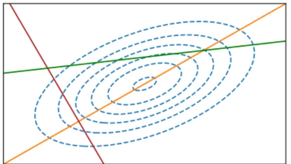
4. Approximating distribution singularities

Both the Bernoulli and Gaussian dropout can be seen as members of a larger family of algorithms where individual layer inputs are perturbed by elementwise i.i.d. random noise. This is equivalent to multiplying the corresponding rowwiof the subsequent weight matrix by the same noise

variable. One could thus definewi = siθi,si ∼ Q(si),

4_{Louizos et al.}₍₂₀₁₇_{) made promising progress there.}

Figure 4.Illustration of approximating distribution singularities. On the left, blue is the standard and orange a correlated Gaussian density. Null sets, are (Borel) sets with zero measure under a distribution. Since both distributions have the same null sets, they are absolutely continuous w.r.t. each other. On the right, orange now represents a degenerate Gaussian supported on a line. Blue assigns zero probability to the line whereas orange assigns all of its mass; orange assigns probability zero to any set excluding the line but blue does not. Hence neither is absolutely continuous w.r.t. the other, and thus KL-divergence is undefined.

Q(si)being an arbitrary distribution, and treat the induced

distribution overwias an approximate posteriorQ(wi).

An issue with this approach is that it leads to unde-fined KL (Q(W)kP(W|X,Y))whenever the prior as-signs zero mass to the individual directions defined byθ. To understand why, note thatKL (Q(W)kP(W|X,Y)) is defined only if Q(W) is absolutely continuous w.r.t. P(W|X,Y)which means that wheneverP(W |X,Y) assigns probability zero to a particular set,Q(W)does so too. The right-hand side plot in Figure4shows a simple example of the case where neither distribution is absolutely continuous w.r.t. the other: the blue Gaussian assigns zero mass to any set with Lebesgue measure zero, such as the line along which the orange distribution places all its mass, and thus the orange Gaussian distribution is not absolutely con-tinuous w.r.t. the blue one. This example is relevant to our problem from above, whereQ(wi)always assigns all its

mass to along the direction defined by the vectorθi. For

more details, see for example (Matthews,2016, Section 2.1). When a measure is not absolutely continuous w.r.t. another measure, it can be shown to have a so calledsingular com-ponent relative to that measure, which we use as a shorthand for referring to this issue. Consequences for variational Bayesian interpretations of dropout are discussed next. 4.1. Implications for Bayesian dropout interpretations Section 3.2 in (Kingma et al.,2015) proposes to use a shared Gaussian random variable for whole rows of the posterior weight matrices. Specificallysi ∼ N(1, α)is substituted

forQ(si)in the generic algorithm described in the previous

section. We call such behaviour in the context of varia-tional inference anapproximating distribution singularity. The singularity has two possible negative consequences.

(6)

First, if only thesiscalars are treated as random variables,

θbecome parameters of the discriminative model instead of the variational distribution. Optimisation of the ELBO will yield a valid Bayesian posterior approximation for thesi.

The lack of regularisation of θ might lead to significant overfitting though, asθrepresent all weights in the BNN. Second, if the fully factorised log uniform prior is used as before, then the directions defined byθconstitute a measure zero subspace ofRD, and thus theKL (Q(W)kP(W))and

consequently KL (Q(W)kP(W|X,Y)) are undefined for any configuration ofθ. This is an instance of the is-sue described in the previous section. As a consequence, standard variational inference with this approximating fam-ily and target posterior is impossible.

A similar problem is encountered in (Gal & Ghahramani, 2016;Gal,2016). The approximate posterior is defined as Q(wi) =p δ0+ (1−p)δθi for each row in every weight matrix. The assumed prior is a product of independent non-degenerate Gaussian distributions which by definition assigns non-zero mass only to sets of positive Lebesgue measure. Again, the approximate posterior is not absolutely continuous w.r.t. the prior and thus the KL is undefined. To address this issue,Gal & Ghahramani(2016) propose to replace the Dirac deltas inQ(wi)by Gaussian distributions

with small but non-zero noise (we call this theconvolutional approach). As an alternative,Gal(2016) proposes to instead discretise the Gaussian prior and the approximate posterior so both assign positive mass only to a shared finite set of values. Because the discretised Gaussian assigns non-zero mass to all points in the set, the approximate posterior is absolutely continuous w.r.t. this prior (we refer to this as thediscretisation approach).

Strictly speaking, the two approaches cannot be equivalent because the corresponding random variables take values in distinct measurable spaces (RDand a discrete grid

re-spectively). Notwithstanding, both approaches are claimed to lead to the same optima for the variational parameters.5 The suggested method for addressing this discrepancy is to introduce acontinuous relaxation(Gal,2016, p. 119) of the optimisation problem for the discrete case. The precise details of this relaxation are not given. One could define it as the relaxation that satisfied the requiredKL-condition(Gal, 2016, Appendix A), but there is of course then a risk of a circular argument. Putting these intuitive arguments on a firmer footing is one motivation for what follows here. In the light of Section3.2, it is natural to ask whether either of the proposed approaches will tend to a stable objective as the added noise shrinks to zero, and the discretisation becomes increasingly refined, respectively for the

convolu-5

Modulo the Euclidean distance to a closest point in the finite set for the discretisation approach.

tional and discretisation approaches. Theorem4provides an affirmative answer by proving that both approaches lead to the same limit under reasonable assumptions.6

Theorem 4. Let Q,P be Borel probability measures on

RD,Pwith a continuous densitypw.r.t. theD-dimensional

Lebesgue measure, andQsupported on an at most count-able measurcount-able setS ⊂_QD_{, with density}_q_{w.r.t. the}

count-ing measure onQD. IfS is infinite, further assume that

diam(S)<∞, i.e.sup_x,y_∈_Skx−yk2<∞.

Then there exists a sequence(s(n))⊂Rindependent ofQ

andPs.t. the limit for both the sequences of convolved and discretised distributions{(Q(n)_,_P(n)_)} n∈N, 7 lim n→∞ n KL (Q(n)kP(n))−s(n)o=E Q log q p , (6)

given the perturbation noise is Gaussian and eventually shrinks to zero, and that the discretisation creates ever finer grid with equally sized cells as n → ∞. The sequence

(s(n)₎_{tends to 0 if}_Q_P_{and to infinity otherwise.}

The right-hand side (r.h.s.) of Equation (6) satisfiesGal’sKL condition, i.e. it leads to the same optimisation problem and thus unifies the convolutional and discretisation approach. Unlike in (Gal,2016, Appendix A), our derivation does not make an extraneous assumption on the distribution over any function of theθparameters nor does it require that the ex-pectation ofkθik2₂grows without bounds withdim(θi).

Nei-ther of these two assumptions is sure to hold in practice as θare being optimised, andθiin any modern (B)NN is

ini-tially scaled bypdim(S)exactly to achieve approximately constant Euclidean norm irrespective of the dimension. We explored whether Equation (6) holds more generally. Theorem5extends the convolutional approach to a consid-erably larger class of approximating distributions.

Theorem 5. LetQ,Pbe Borel probability measures on_RD_,

Pwith a bounded continuous densitypw.r.t. the Lebesgue measure onRD, andQsupported on a measurable linear

manifoldS⊂RDof (Hamel) dimensionKS. AssumeQhas

a continuous bounded densityqw.r.t. the Lebesgue measure onS, where the continuity is w.r.t. the trace topology. Then there exists a sequence(s(n))⊂Rdependent only on

KSs.t. the following holds for the convolutional approach,

lim n→∞ n KL (Q(n)kP(n))−s(_Kn) S o =_E Q log q p , (7)

given the perturbation noise is Gaussian and eventually shrinks to zero. The sequence(s(_Kn)

S)tends to 0 ifQP

and to infinity otherwise.

6

We state only the most important assumptions in Theorems4

and5.Please see the appendix for the full set of assumptions.

7_P(n)_{= P}_,_∀_n_∈

(7)

A result related to Theorem5for the discretisation approach can be derived under assumptions similar to Theorem4with one important difference:(s(_Kn)

S), if it exists, is affected not only byKS, but also by the orientation ofSinRD. This

is because the dominating Lebesgue measure is different for each affine subspaceSand thus, unlike in the countable support case,qcannot be defined w.r.t. a single dominating measure. Implicit in Theorems4and5is that the same constant can be subtracted from KL (Q(n)_k_P(n)₎_{for all}

distributionsQwith the same type of support. Hence if we are optimising over a family of singular approximating distributions, the sequence (s(n)₎_(resp. _(s(n)

KS)) does not need to change between updates to obtain the desired limit. Before moving to Section 5 which discusses some of the merits of using Equations (6) and (7) as an objective for approximate Bayesian inference, let us make two comments. First, taking the limit makes the decision about size of per-turbation or coarseness of the discretisation unnecessary. The sequences used do not cause the same instability prob-lems discussed in Section3.2because the true posterior is well-defined even in the limit, which we assume in saying thatPis a probability measure. The main open question is thus whether optimisation of the r.h.s. of Equation (6) will yield a sensible approximation of this posterior.

Second, if there is a family of approximate posterior distri-butionsQparametrised byψ∈Ψ, the equality,

argmin ψ∈Ψ QEψ logqψ p = lim n→∞argmin_ψ_∈_Ψ KL (Q (n) ψ kP (n)₎_, (8) need not hold unless stricter conditions are assumed. Equa-tion (8) is of interest in cases whenKL (Q(_ψn)kP(n)₎_has

some desirable properties (e.g. good predictive performance) which we would like to preserve. However, this is not the case for variational Bernoulli dropout as the objective being used byGal & Ghahramani(2016) is, in terms of gra-dients w.r.t. the variational parameters, identical to the limit. Furthermore, we can view both the discretisation and con-volutional approaches as mere alternative vehicles to derive the same quasi discrepancy measure (cf. Section5). If this quasi discrepancy possesses favourable properties, the pre-cise details of optima attained along the sequence might be less important. One benefit of this view is in avoiding arguments like the previously mentionedcontinuous relax-ation(Gal,2016, p. 119).

5. Quasi-KL divergence

The r.h.s. of Equations (6) and (7) is markedly similar to the formula for standard KL divergence. We now make this link explicit. IfZPS :=

R

SpdmS < ∞,mS being

either the counting or the Lebesgue measure dominating

measure forq, we can the probability densitypS :=p/ZPS, and denote the corresponding distribution on(S,BS)byPS.

We term Equation (9) theQuasi-KL(QKL) divergence, QKL (QkP) :=E Q log q p = KL (QkPS)−log ZPS. (9) Taking Equation (9) as a loss function says that we would like to find such aQfor which the KL divergence between QandPS is as small as possible, while making sure that

the corresponding setSruns through high density regions ofP, preventingQfrom collapsing to subspaces wherepis easily approximated byqbut takes low values. Sincepis continuous (c.f. Theorem4), values ofproughly indicate how much massPassigns to the region whereSis placed. Standard KL divergence and QKL are equivalent when Q Pand the two distributions have the same support. QKL is not a proper statistical divergence though, as it is lower bounded by−log ZPS instead of zero. The non-negativity could have been satisfied by defining QKL as KL (QkPS), dropping thelog ZPS term. However, this would mean losing the above discussed effect of forcing S to lie in a relatively high density region ofP, and also the motivation of being a limit of the two sequences consid-ered in Theorem4.

Nevertheless, QKL inherits some of the attractive properties of KL divergence: the densitypneed only be known up to a constant, the reparameterisation trick (Kingma & Welling, 2014) and analogical approaches for discrete random vari-ables (Maddison et al.,2017;Jang et al.,2017;Tucker et al., 2017) still apply, and stochastic optimisation and integral approximation techniques can be deployed if desired. On a more cautionary note, we emphasise thatEQ(logpq)is

upper bounded bylog ZPS and not the log marginal likeli-hood as is the case for standard KL use in VI. Hence optimi-sation of this objective w.r.t. hyperparameters ofPneed not work very well, since the resulting estimates could be biased towards regions where the variational family performs best.8 This might explain why prior hyperparameters usually have to be found by validation error based grid search (Gal,2016, e.g. p. 119) instead of ELBO optimisation as is common in the sparse Gaussian Process literature (Titsias,2009). Whether and when is QKL an attractive alternative to the more computationally expensive but proper statistical discrepancy measures which are capable of handling sin-gular distributions (e.g. Wasserstein distances) is beyond the scope of this paper. To provide basic intuition of whether QKL might be a sensible objective for inference, Section5.1 focuses on a simple practical example that yields a well known algorithm as the optimal solution to QKL optimisa-tion, and exemplifies some of the above discussed behaviour. 8_{A similar issue for KL was observed by}_{Turner et al.}₍₂₀₁₀_).

(8)

5.1. QKL and Principal Component Analysis Proposition6is an application of Theorem5:

Proposition 6. AssumeP =N(0,Σ),Σa (strictly) posi-tive definite matrix of rankD, with a degenerate Gaussian

Q =N(0,AV AT), whereAis aD×Kmatrix with or-thonormal columns, andV is aK×K(strictly) positive definite diagonal matrix. Then,

QKL (QkP) = c−1 2 K X k=1 logVkk+ 1 2Tr ATΣ−1AV

wherecis constant w.r.t.A,V. The optimal solutionA,V

is to set columns ofAto the topKeigenvectors ofΣand the diagonal ofV to the corresponding eigenvalues.9

Proposition6shows that the QKL-optimal way to appro-ximate a full rank Gaussian with a degenerate one is to perform PCA on the covariance matrix. The result is intu-itively satisfying as PCA preserves the directions of highest variance;Swas thus indeed forced to align with the high-est density regions underPas suggested in Section5. See Figure5for a visualisation of this behaviour. Proposition7 presents a variation of the result ofTipping & Bishop(1999), showing that Equation (8) can hold in practice.

Proposition 7. Assume similar conditions as in Propo-sition 6, except Q will now be replaced with a series of distributions convolved with Gaussian noise: Q(n) = N(0,A(n)V(n)(A(n))T+τ(n)I). Given τ(n) ↓ 0 as

n→ 0and the obvious constraints onA(n),V(n), Equa-tion(8)holds in the sense of shrinking Euclidean/Frobenius norm between{A(n)_,_V(n)_}

and the PCA solution.

It is necessary to mention that both the QKL from Propo-sition6and any of the yet unconverged KL divergences in Proposition7have D_Klocal optima for any combination of the eigenvectors which might lead to potentially problem-atic behaviour of gradient based optimisation.

6. Conclusion

The original intent behind dropout was to provide a sim-ple yet effective regulariser for neural networks. The main value of the subsequent reinterpretation as a form of appro-ximate Bayesian VI thus arguably lies in providing a prin-cipled theoretical framework which can explain the empi-rical behaviour, and guide extensions to the method. We have shown the current theory behind variational Bayesian dropout to have issues stemming from two main sources: 1) use of improper or pathological priors; 2) singular approxi-mating distributions relative to the true posterior.

9

We have assumed both Gaussians are zero mean to simplify the notation. Analogical results holds in the more general case.

Figure 5.Visualisation of the relationship between QKL minimisa-tion and PCA. The target in this example is the blue two dimen-sional Gaussian distribution. The approximating family is the set of all Gaussian distributions concentrated on a line, which would be problematic with conventional VI (c.f. Section4). For all of the linear subspaces shown by the coloured lines the KL term on the right hand side of Equation (9) can be made zero by a suitable choice of the normal mean and variance. The remaining term

−log ZPS therefore dictates the choice of subspace. The orange

line is optimal aligning with the largest eigenvalue PCA solution.

The former issue pertains to the improper log uniform prior in variational Gaussian dropout. We proved its use leads to irremediably pathological behaviour of the true posterior, and consequently studied properties of the optimisation ob-jective from a non-Bayesian perspective, arguing it is set up in such a way that cancels some of the pathologies and can thus still provide good empirical results, albeit not because of the Bayesian or the related MDL arguments.

The singular approximating distribution issue is relevant to both the Bernoulli and Gaussian dropout by making stan-dard VI impossible due to an undefined objective. We have shown that the proposed remedies in (Gal & Ghahramani, 2016; Gal,2016) can be made rigorous and are special cases of a broader class of limiting constructions leading to a unique objective which we termed quasi-KL divergence. We presented initial observations about QKL’s properties, suggested an explanation for the empirical difficulty of ob-taining hyperparameter estimates in dropout-based approxi-mate inference, and motivated future exploration of QKL by showing it naturally yields PCA when approximating a full rank Gaussian with a degenerate one.

As use of improper priors and singular distributions is not isolated to the variational Bayesian dropout literature, we hope our work will contribute to avoiding similar pitfalls in future. Since it relaxes the standard KL assumptions, QKL will need further careful study in subsequent work. Nevertheless, based on our observations from Section 5 and the previously reported empirical results of variational Bayesian dropout, we believe QKL inspires a promising future research direction with potential to obtain a gen-eral framework for the design of computationally cheap optimisation-based approximate inference algorithms.

(9)

Acknowledgements

We would like to thank Matej Balog, Diederik P. Kingma, Dmitry Molchanov, Mark Rowland, Richard E. Turner, and the anonymous reviewers for helpful conversations and valu-able comments. Jiri Hron holds a Nokia CASE Studentship. Alexander Matthews and Zoubin Ghahramani acknowledge the support of EPSRC Grant EP/N014162/1 and EPSRC Grant EP/N510129/1 (The Alan Turing Institute).

References

Gal, Y.Uncertainty in Deep Learning. PhD thesis, Univer-sity of Cambridge, 2016.

Gal, Y. and Ghahramani, Z. Dropout as a Bayesian Ap-proximation: Representing Model Uncertainty in Deep Learning. In Balcan, M. F. and Weinberger, K. Q. (eds.),

Proceedings of The 33rd International Conference on Ma-chine Learning, volume 48 ofProceedings of Machine Learning Research, pp. 1050–1059, New York, New York, USA, 20–22 Jun 2016. PMLR.

Hron, J., Matthews, Alexander G. de G., and Ghahramani, Z. Variational Gaussian Dropout is not Bayesian. In Sec-ond workshop on Bayesian Deep Learning (NIPS 2017). 2017.

Jang, E., Gu, S., and Poole, B. Categorical Reparame-terization with Gumbel-Softmax. 2017. URLhttps: //arxiv.org/abs/1611.01144.

Johnson, S. G. Faddeeva Package. http:

//ab-initio.mit.edu/wiki/index.php/ Faddeeva_Package, 2012.

Kingma, D. P. and Welling, M. Auto-Encoding Variational Bayes. InProceedings of the Second International Con-ference on Learning Representations (ICLR 2014), April 2014.

Kingma, D. P., Salimans, T., and Welling, M. Variational Dropout and the Local Reparameterization Trick. In Cortes, C., Lawrence, N. D., Lee, D. D., Sugiyama, M., and Garnett, R. (eds.),Advances in Neural Information Processing Systems 28, pp. 2575–2583. Curran Asso-ciates, Inc., 2015.

Louizos, C., Ullrich, K., and Welling, M. Bayesian com-pression for deep learning. In Guyon, I., Luxburg, U. V., Bengio, S., Wallach, H., Fergus, R., Vishwanathan, S., and Garnett, R. (eds.),Advances in Neural Information Processing Systems 30, pp. 3290–3300. Curran Asso-ciates, Inc., 2017.

Maddison, C. J., Mnih, A., and Teh, Y. W. The Concrete Distribution: A Continuous Relaxation of Discrete

Ran-dom Variables. InInternational Conference on Learning Representations (ICLR), 2017.

Matthews, Alexander G. de G.Scalable Gaussian process inference using variational methods. PhD thesis, Univer-sity of Cambridge, 2016.

Matthews, Alexander G. de G., Hron, J., Rowland, M., Turner, R. E., and Ghahramani, Z. Gaussian Pro-cess Behaviour in Wide Deep Neural Networks. In-ternational Conference on Learning Representations,

2018. URLhttps://openreview.net/forum?

id=H1-nGgWC-.

Molchanov, D., Ashukha, A., and Vetrov, D. Variational Dropout Sparsifies Deep Neural Networks. In Proceed-ings of the 34th International Conference on Machine Learning, volume 70 ofProceedings of Machine Learn-ing Research, pp. 2498–2507. PMLR, 2017.

Neal, R. M. Bayesian Learning for Neural Networks. Springer-Verlag New York, Inc., Secaucus, NJ, USA, 1996.

Neklyudov, K., Molchanov, D., Ashukha, A., and Vetrov, D. P. Structured Bayesian Pruning via Log-Normal Multi-plicative Noise. In Guyon, I., Luxburg, U. V., Bengio, S., Wallach, H., Fergus, R., Vishwanathan, S., and Garnett, R. (eds.),Advances in Neural Information Processing Sys-tems 30, pp. 6778–6787. Curran Associates, Inc., 2017. Srivastava, N., Hinton, G. E., Krizhevsky, A., Sutskever, I.,

and Salakhutdinov, R. Dropout: A Simple Way to Prevent Neural Networks from Overfitting. Journal of Machine Learning Research, 15(1):1929–1958, 2014.

Tibshirani, R. Regression Shrinkage and Selection via the Lasso. Journal of the Royal Statistical Society. Series B (Methodological), pp. 267–288, 1996.

Tipping, M. E. and Bishop, C. M. Probabilistic Principal Component Analysis. Journal of the Royal Statistical Society: Series B (Statistical Methodology), 61(3):611– 622, 1999.

Titsias, M. K. Variational learning of inducing variables in sparse Gaussian processes. InProceedings of the 12th International Conference on Artificial Intelligence and Statistics, pp. 567–574, 2009.

Tucker, G., Mnih, A., Maddison, C. J., Lawson, J., and Sohl-Dickstein, J. REBAR: Low-variance, unbiased gradient estimates for discrete latent variable models. In Guyon, I., Luxburg, U. V., Bengio, S., Wallach, H., Fergus, R., Vishwanathan, S., and Garnett, R. (eds.),Advances in Neural Information Processing Systems 30, pp. 2624– 2633. Curran Associates, Inc., 2017.

(10)

Turner, R. E., Berkes, P., and Sahani, M. Two problems with variational expectation maximisation for time-series models. Inference and Estimation in Probabilistic Time-Series Models, 2010.

(11)

Jiri Hron1 Alexander G. de G. Matthews1 Zoubin Ghahramani1 2

A. Proofs for Section

3

Notation and identities used throughout this section:ψ(x) for the digamma function,ψ(x+ 1) =ψ(x) + 1/x,ψ(k+ 1) = Hk−γwhereHkis thekthharmonic number andγis

the Euler–Mascheroni’s constant,Ei(x) =−R∞

−xe

−t_/t_dt

is the exponential integral function, P∞ k=1u

k_H k/k! =

eu_(γ_+log_u₋_Ei(₋_u))₍_{Dattoli & Srivastava}_,₂₀₀₈_;_Gosper_, 1996), andP∞

k=1u

k_/(k!_{k) = Ei(u)}₋_γ₋_log_u₍_Harris_, 1957); the last two identities hold foru >0. Importantly, we define00_{:= 1}_{unless stated otherwise.}

Proof of Proposition1. Denote the likelihood value by > 0. Take an arbitrary numberrsuch that > r > 0. By continuity, we can findδ >0such that|w−0|< δimplies that the likelihood value is greater thanr; letA30denote the open ball of radiusδcentred at 0. Because both the prior density and the likelihood function only take non-negative values, we can apply the Tonelli–Fubini’s theorem to obtain,

Z = Z RD−1 p(W¬w) " Z R p(w)p(Y |X,W) dw # dW¬w > Z RD−1 p(W¬w) " Z A C |w|rdw # dW¬w=∞,

whereW¬w is a shorthand forW \w. WhenZ = ∞,

the measure ofRDunderP(W|X,Y)is infinite and thus it cannot be a proper probability distribution.

Proof of Proposition2. Using standard identities about Gaussian random variables, and the fact that v := ε2_,

ε∼ N(µ/σ,1), follows the non-central chi-squared distri-butionχ2_{(λ, ν)}_with_ν _{= 1}_{degrees of freedom and}

non-centrality parameterλ= (µ/σ)2_{, we have,}

E Q(w)[logq(w)]−Q(Ew)[logp(w)] = E Q(w)[logq(w)]−log C + 1 2Q(Ew)[log|w| 2 ] 1

Department of Engineering, University of Cambridge, Cam-bridge, United Kingdom2Uber AI Labs, San Francisco, California, USA. Correspondence to: Jiri Hron<[email protected]>. Proceedings of the35th

International Conference on Machine Learning, Stockholm, Sweden, PMLR 80, 2018. Copyright 2018 by the author(s). = c1+ 1 2ε∼N(Eµ/σ,1)[logσ 2_ε2_] = c1+ 1 2 logσ2+ E v∼χ2₍_µ2_/σ2_,₁₎[logv] = c2+ 1 2 Z ∞ 0 ∞ X k=0 e− µ2 2σ2( µ2 2σ2) k k! vk−1 2e− v 2 2k+1 2Γ(k+1 2) logvdv ,

wherec1:=−1₂log(2πeσ2)−log C,c2:= c1+1₂log(σ2),

and we used the fact thatχ2_{(λ, ν)}_{is equivalent to a Poisson}

mixture of centralised chi-squared distributions. Define,

fn(v) := n X k=0 e− µ2 2σ2 (₂µ_σ22)k k! vk−1 2e−v2 2k+1 2Γ(k+1 2) logv ,

and rewrite the last integral as,

Z ∞ 0 lim n→∞fn(v)dv = Z 1 0 lim n→∞fn(v)dv+ Z ∞ 1 lim n→∞fn(v)dv . Observe thatfn ≥ 0,∀n ∈ N, andfn ↑ f∞ pointwise onv ∈ [1,∞), andfn <0,∀n ∈N, andfn ↓ f∞ point-wise onv ∈[0,1), forf∞defined as the pointwise limit offn. Hence we can use the monotone convergence

the-orem as long as the|R

f0(v)dv|<∞. Using the identity

Ev∼χ2₍₀_,ν₎[logv] =ψ(ν/2)−log(1/2), we have,

Z ∞ 0 fn(v)dv= log 2 + e −µ2 2σ2 n X k=0 (₂µ_σ22)k k! ψ(1/2 +k), which means that fn ∈ L1,∀n ∈ N. Because both

R1

0 |fn(v)|dv and R∞

1 |fn(v)|dv are upper-bounded by R∞

0 |fn(v)|dv, we can apply the monotone convergence

theorem to equate, Z 1 0 lim n→∞fn(v)dv= limn→∞ Z 1 0 fn(v)dv Z ∞ 1 lim n→∞fn(v)dv= limn→∞ Z ∞ 1 fn(v)dv ,

and thus by Theorem 4.1.10 in (Dudley,2002) conclude

R∞ 0 f∞(v)dv= limn→∞ R∞ 0 fn(v)dv. Substituting back, E Q(w) [logq(w)]− _E Q(w) [logp(w)]

(12)

= c2+ 1 2 log 2 + e− µ2 2σ2 ∞ X k=0 (₂µ_σ22) k k! ψ(1/2 +k) = c3− 1 2 ∂M(a; 1/2;−µ2/(2σ2)) ∂a _a₌₀ ,

whereM(a;b;z)denotes the Kummer’s function of the first kind, and c3 := c2− 3₂log 2− 1₂γ. It is easy to check

that Equation (3) holds for allu= 0assuming00_{= 1}_.

The last equality above was obtained using Wolfram Al-pha (Wolfram—Alpha,2017b). To validate this result, we performed an extensive numerical test, and will now show that the series indeed converges foru=µ2/(2σ2)∈[0,∞), i.e. for all plausible values ofu. The comparison test gives us convergence foru∈(0,∞): ∞ X k=0 uk k!ψ(1/2 +k)< ψ(1/2) + ∞ X k=1 uk k!ψ(1 +k) =ψ(1/2) + ∞ X k=1 uk k!(Hk−γ)

=ψ(1/2) + eu(γ+ logu−Ei(−u))−γ(eu−1) =ψ(1/2)−γ+ eu(logu−Ei(−u)),

where we use the fact that the individual summands are non-negative fork≥1(which is also means we need not take the absolute value explicitly). It is trivial to check that the series converges atu= 0, and thus we have convergence for allu∈[0,∞).

To obtain the derivative with respect tou, we use the infi-nite series formulation from Equation (3), and the fact that the derivative of a power series within its radius of conver-gence is equal to the sum of its term-by-term derivatives (see (Gowers,2014) for a nice proof). Using that only the infinite series in Equation (3) depends onu, we obtain,

∇ue−u ∞ X k=0 uk k!ψ(1/2 +k) =∇u e−uψ(1/2) + e−u ∞ X k=1 uk k!ψ(1/2 +k) = −e−uψ(1/2) + e−u ∞ X k=1 _uk−1 (k−1)!ψ(1/2 +k) −e−u ∞ X k=1 _uk k!ψ(1/2 +k) = e−u(ψ(3/2)−ψ(1/2)) + e−u ∞ X k=1 _uk k!ψ(3/2 +k) −e−u ∞ X k=1 _uk k!ψ(1/2 +k) = 2e−u+ e−u ∞ X k=1 uk k! 1 1/2 +k = e −u ∞ X k=0 uk k! 1 1/2 +k = 2D+( √ u) √ u ,

foru >0and is equal to2ifu= 0; in our case, the condi-tionu≥0is satisfied by definition; to obtain the expression in Equation (5), notice that the above series is multiplied by1/2in Equation (3). Equality of the last infinite series to2D+(

√

u)/√u, was again obtained using Wolfram Al-pha (Wolfram—Alpha,2017a); the result was numerically validated, and convergence onu ∈ (0,∞)can again be established using the comparison test:

∞ X k=0 uk k! 1 1/2 +k = ∞ X k=0 uk k! 1 1/2 +k <2 + ∞ X k=1 uk k! 1 k = 2 + Ei(u)−γ−logu .

The convergence atu = 0is obtained trivially, yielding convergence for allu∈[0,∞).

D+(u)and √

uare continuous on(0,∞), and √u > 0; henceD+(u)/

√

uis continuous on(0,∞), and from defi-nition of the Dawson integrallimu→0+D+(

√

u)/√u= 1, i.e. the gradient is continuous inuon[0,∞).

Proof of Corollary3. We use the conclusion of Proposi-tion2which established differentiability foru ∈ [0,∞) (and thus continuity on the same interval). To show that KL (Q(w)kP(w))is strictly increasing foru∈[0,∞), it is sufficient to observe, ∇uKL (Q(w)kP(w)) = 1 2e −u ∞ X k=0 uk k! 1 1/2 +k >0, because each summand is strictly positive foru∈[0,∞) (given00= 1). By a simple application of the mean value theorem, we concludeKL (Q(w)kP(w))is strictly increas-ing inuon[0,∞).

B. Proofs for Section

4

Throughout this section, let (_RD_,_k·k

2) be the D

-dimensional Euclidean metric space,T the usual topology, andBthe corresponding Borelσ-algebra. Letλd_,_d _∈

N, be the d-dimensional Lebesgue measure.1 _P,_Q_{will be}

probability measures, Pwith continuous density pw.r.t. the Lebesgue measure onRD, andQconcentrated on some S∈ B, which is either (at most) countable or a linear mani-fold. LetKSbe the Hausdorff dimension ofS, i.e. zero in

1

More precisely the restriction of them-dimensional Lebesgue measure to the corresponding Borelσ-algebra. We will be using the term Lebesgue measure instead of the sometimes used term Borel measurewhich we use to refer to any measure defined on the Borelσ-algebra.

(13)

the countable, anddim(S)in the linear manifold case (dim being the Hamel dimension). The restrictionQ|S ofQto

(S,BS),BSthe traceσ-algebra, will be denoted byQe.

AssumeQehas a densityqw.r.t. the counting measure onQD

ifSis at most countable,2or w.r.t. Lebesgue measure onS in the linear manifold case. In the (at most) countable case, further assume thatdiam(S)<∞ifSis infinite (trivially true ifSis finite). IfSis a linear manifold, assume thatqis continuous w.r.t. the trace topologyTS, and that bothqand

pare bounded; denote the bounds on densitiesqandpby CqandCprespectively. We will be usingmSas a shorthand

for either of the corresponding dominating measures ofq. We will also assume thatlogq∈L1₍

e

Q). Finally, the axiom of choice is assumed throughout.

We will be using the following fact: because (RD,k·k2)

is a complete separable metric space, every finite Borel measure is regular by Ulam’s theorem (Dudley,2002, The-orem 7.1.4), and thus tight by definition. Hence for any probability measurePon(RD,B)and everyε >0, there exists a compact setC∈ Bs.t.P(C)>1−ε.

The proofs of Theorems4and5will be divided into multiple propositions, each proven in a subsection corresponding to the limiting construction used.

Proof of Theorem4. Combine Propositions8and21.

Proof of Theorem5. Use Proposition9.

Notice that the statements of Propositions8,9and21 dif-fer slightly from those of Theorems4and5by denoting the limit asEQelog

q

p|S instead ofEQlogq_p. The former is

more precise in the sense thatqis the density ofQe w.r.t.

mS on(S,BS), and thus is not measurable w.r.t.Q, making

the integral ill-defined. After swappingQforQe, the

inter-change ofpforp|S is necessary for similar reasons. We

omitted this detail from the main text so as to meet the page limit, and to lighten the technicality of the discussion. B.1. Convolutional approach

Before approaching the proof of Propositions8and9, we note that Lemma11allows us to assume thatS=RKS _×

{0}D−KS _if_S_{is a linear manifold w.l.o.g.}

The following definitions will be useful: letZ andE be independent random variables respectively distributed ac-cording to the distributionsPE :=N(0, ID)andQ. Define

the shorthandsE(n)_:=_E_/√_n_and_Z(n) _:=_Z₊_E(n)_{. We}

further define the random variablesEe:=E (n) 1 : KS×{0}

D−KS_,

2

We use the countable measure on rationals to avoid having to deal with a dominating measure that is notσ-finite.

where the subscript denotes the firstKSelements of the

vec-tor (Ee(n) = 0ifKS = 0),Ee(n) := Ee/ √

n, andZe(n) :=

Z+Ee(n). The corresponding distributions will be denoted as

follows:Q(n)_{= Law(Z}(n)₎_, e Q(n)_{:= Law(} e Z(n)₎_,_P(n) E := Law(E(n)₎_,_P e E := Law(Ee), andP (n) e E := Law(Ee (n)₎_. Notice that(Z, Z(n)_, e Z(n)₎_and₍_E(n)_, e E(n)₎_are

determin-istically coupled collections of random variables. Also ob-serve that we only convolve the approximating distribu-tion with the Gaussian noise, and not the targetP. Hence P(n)_{= P,}_∀_n_∈

N; we will thus omit the superscript here. The convolution of two Borel measuresµ, νonRd,d∈N, will be denoted by µ ? ν where for any measurable set B, (µ ? ν)(B) = Rµ(B −x)ν(dx). Observe Q(n) = Q?N_RD(0, n−1I), and Qe(n) = Qe?NS(0, n−1I) with NS(0, n−1I) = P

(n)

e

E being the Gaussian probability mea-sure on (S,BS) (assumingNS(µ,Σ) = δµ, the Dirac’s

delta distribution, ifSat most countable). As a corollary of (Dudley,2002, Proposition 9.1.6), we have,

q(n)(x) =

Z

φλ_x,nD−1_IqdmS , x∈RD, (10)

whereφλ_µ,D_Σis the density function w.r.t.λDofN(µ,Σ)(we will omit the superscript unless confusion may arise). By an analogous argument, we obtain,

e q(n)(x) = Z φmS x,n−1IqdmS , x∈S , (11) whereφmS µ,Σ(z) =δKr(z−µ)ifSis at most countable (δKr

is the Kronecker’s delta function), asmS is the counting

measure andNS(µ,Σ) =δµ(see above), and the usual

den-sity function of degenerate Gaussian ifmS is the Lebesgue

measure onS. Notice that it would have been more pre-cise to replaceφλ_x,nD−1_Iin Equation (10) withφ

λD

x,n−1_I|S(c.f.

Lemma22); we omit the restriction in situations where its necessity is clear from the context.

Proposition 8. LetSbe at most countable and all the rel-evant aforementioned assumptions hold. We consider two cases:logp∈L1(Q)andlogp /∈L1(Q). Iflogp∈L1(Q), assume that the random variables {logp(Z(n))}n∈Nare uniformly integrable.3 Then, lim n→∞ n KL (Q(n)kP)−s(n)o=E e Q log q p|S , withs(n)_:=₋D 2 log(2πen −1₎_.

Proof of Proposition8. First, assume thatlogp ∈ L1_(Q)_.

Becauselogq∈L1₍ e

Q)by assumption, we havelog_pq_|S ∈ 3_{A useful sufficient condition is provided in Proposition}₁₀_.

(14)

L1₍ e

Q)by Lemma22and (Dudley,2002, Theorem 4.1.10). We can thus focus on convergence of the cross-entropy and negative entropy terms individually. By Lemma12, the cross-entropy term converges. The negative entropy term converges by Lemma13.

It remains to investigate the caselogp /∈L1(Q). Because Lemma13 still holds, we can invoke Lemma 20 which establishes that both the sequence(KL (Q(n)kP)−s(n)) and the integralEQelog

q

p|S do not converge as desired. Proposition 9. LetSbe a linear manifold and all the rel-evant aforementioned assumptions hold. We consider two cases:logp∈L1_(Q)_and_log_{p /}_∈_L1_(Q)_{. If}_log_p_∈_L1_(Q)_,

assume that the random variables {logp(Z(n)₎_} n∈Nare uniformly integrable,4_{and that}

EkZk22<∞. Then, lim n→∞ n KL (Q(n)kP)−s(_Kn) S o =E e Q log q p|S , withs(_Kn) S :=− D−KS 2 log(2πen −1₎_.

Proof of Proposition9. First, assume thatlogp ∈ L1(Q). Becauselogq∈L1₍

e

Q)by assumption, we havelog_pq_|S ∈

L1₍ e

Q)by Lemma22and (Dudley,2002, Theorem 4.1.10). We can thus focus on convergence of the cross-entropy and negative entropy terms individually.

By Lemma12, the cross-entropy term converges. Turning to the negative entropy term, by Lemma14, we need to prove,

Elogqe (n)₍

e

Z(n))→Elogq(Z).

Lemma15giveslogq_e(n)(Ze(n))→logq(Z)a.s. Lemma19

then yields the convergence in mean. Therefore, lim n→∞ n KL (Q(n)kP)−s(_Kn) S o =_E e Q log_pq_|S .

It remains to investigate the caselogp /∈L1(Q). Because Lemmas14and15and thus also Lemma19still hold, we can invoke Lemma20which establishes that both the se-quence(KL (Q(n)_k_P)₋_s(n)₎_{and the integral}

EQelog

q p|S do not converge as desired.

Proposition 10. Forf ∈C(_RD₎_{, a collection of random}

variables {f(Z(n)₎_}

n∈N is uniformly integrable if there exists somer >0s.t.∀x∈RDwithkxk2 > r,|f(x)| ≤ hp(x)wherehp: RD →R,x7→Ppj=1cjkxk

j

2, for some

c1, . . . , cp∈R, andEkZkp2<∞.

5

4_{A useful sufficient condition is provided in Proposition}₁₀_. 5

Proposition10can be straightforwardly extended to polynomi-als in anyp-normkxkp= (PD_i₌₁xpi)

1/p

,p∈[1,∞)by strong equivalence of p-norms on finite Euclidean spaces.

Proof of Proposition10. Kallenberg (2006, p. 44, Equa-tion (5)) states that a sequence of integrable random vari-ables{ξn}n∈Nis uniformly integrable iff,

lim

k→∞lim supn→∞ E I|ξn|>k

|ξn|= 0. (12)

Let us first ensure that random variables{f(Z(n))}n∈Nare integrable. DefiningU :={x∈RD: kxk2> r}, E IU f(Z) ≤_{E I}Uhp(Z),

withhp(Z)being a linear combination of termskZ(n)kk2

fork∈0,1, . . . , p. By Cauchy–Bunyakovsky–Schwarz, E IUkZ(n)kk2 ≤EkZ+E/ √ nkk 2 ≤2 3k 2−1 EkZkk2+ 2EkZk k 2 2k E √ nk k 2 2 +Ek E √ nk k 2 . AsEkZkt2 < ∞for allt ∈ [0, p]by H¨older’s inequality

and the assumptionEkZkp2<∞, the second and third

sum-mands will go to0asn→ ∞, and the first term is finite. BecauseE IUC|f(Z(n))| ≤ sup_UC|f| which is finite by continuity of|f|and compactness ofUC(Heine–Borel the-orem), the random variables{f(Z(n))}n∈Nare integrable. By Equation (12), it is sufficient if∀ε >0,∃k∈Rs.t.,

lim sup

n→∞ E I|f(Z

(n)₎_|_>k|f(Z(n))|< ε .

Because any finite collection of integrable random variables is uniformly integrable, we can findδ >0s.t.∀B∈ Bwith Q(B)≤ δ,E IBkZkj2 ≤ ε/(2

3j

2−1|c_j|)forj = 1, . . . , p. We w.l.o.g. assumedcj>0,∀jas otherwise we could just

ignore the corresponding terms.

By tightness ofQ, for everyδ >0there exists a compact set Kδ,αs.t.Q(Kδ,α)>1−δ(the purpose ofαwill become

clear later). Because we are on a finite Euclidean space, Kδ,αis bounded and thus we can w.l.o.g. assumeKδ,α =

¯

Brδ−α(sδ), a closed ball centred atsδ ∈ RDwith radius rδ−α, for someα > 0, s.t.rδ−α > r, i.e.Kδ,αC ⊂U.

ClearlyKδ,α ⊂ Kδ := ¯Brδ(sδ)and thusQ(Kδ) > 1− δ. Define κ = sup_K

δ|f| which is a finite constant by continuity off and compactness ofKδ. We will now show,

lim sup

n→∞ E I|f|>κ

|f(Z(n))|< ε .

By the assumption|f| ≤hponU, we have,

E I|f|>κδ|f(Z (n)₎_{| ≤} E IKC δ|f(Z (n)₎_| ≤ p X j=1 cjE IKC δkZ (n)_kj 2= p X j=1 cjE IKC δkZ+E/ √ nkj₂,

where each of the r.h.s. summands can be upper bounded, 2 3j 2−1 E IKC δkZk j 2+ 2EkZk j 2 2k E √ nk j 2 2 +Ek E √ nk j 2 .

(15)

As before, all but the first term will vanish asn → ∞

and thus we can ignore them in evaluation of thelim sup. Ignoring the multiplicative constants for a moment, we turn our attention to theE IKC

δ(Z

(n)₎_k_Z_kj

2 =E IKC δ(Z+

E/√n)kZkj₂where the noise term remained inside the indi-cator random variable by construction of the upper bound. DefineA(αn) := {x ∈ RD: kxk2 ≤α

√

n} ∈ B,β(n) _:=

PE(A

(n)

α )and observeβ(n)↑1. BecausekZ+E/ √

nk2≤ kZk2 +kE/√nk2 by the triangle inequality, and (Z +

E/√n) ∈ K_δCiffkZ+E/√nk2 > rδ by definition, we haveI_A(n) α (E)IKδC Z+E/ √ n≤I_A(n) α (E)IKδ,αC (Z)for alln∈N. Therefore, E[(I_A(n) α (E) +I(A(αn))C(E))IKCδ(Z+E/ √ n)kZkj₂] ≤_E[_I_A(n) α (E)IK C δ,α(Z)kZk j 2] +E[I(Aα(n))C(E)kZk j 2] =β(n)E[IKC δ,α(Z)kZk j 2] + (1−β (n)₎ EkZkj2.

BecauseEkZkj2<∞by H¨older’s inequality andβ(n)↑1,

the limit and thuslim supof the r.h.s. is clearly, E IKC δ,α(Z)kZk j 2< ε 232j−1|c_j| ,

where the upper bound is by uniform integrability ofkZkj₂

and the construction ofKδ,α. Substituting back,

lim sup

n→∞ E I|f|>k

|f(Z(n))|< ε , for allk≥κwhich concludes the proof. AUXILIARY LEMMAS

Lemma 11. AssumeSis a linear manifold, i.e.S={x∈

RD:x=t(z), z∈S0}, whereS0=RKS×{0}D−KS, and t:x7→b+Axwithb∈_RD_and_A_∈ RD×Dorthonormal. Then, lim n→∞{KL (Q (n)_k_P)₋_s(n)_}₌ E e Q log q p|S , with(s(n)₎_⊂

R, if and only if, lim n→∞{KL ((t −1 # Q)?P (n) E kt −1 # P)−s (n)_} = E t−1 # Qe log q◦t p|S◦t . Furthermore, q◦t= dt −1 # Qe dλS0 , whereλS0 =t −1

# mS is the Lebesgue measure onS0with

the corresponding traceσ-algebraBS0. Ifqis continuous

and bounded, then alsoq◦tis continuous bounded w.r.t. the corresponding trace topology.

Proof of Lemma11. From definition,t−1_{(x) =}_AT_(x₋_b)

which is clearly a homeomorphism from_RD _{onto itself.}

Because we are working with Borelσ-algebras, we can use Lemma 7.5 in (Gray,2011) to establish,

KL (Q(n)kP) = KL (t−_#1Q(n)kt−_#1P).

By definition,t−_#1Q(n)_{= Law(t}−1_(Z+_E(n)₎₎_{; substituting}

t−1_(Z₊_E(n)_{) =}_AT_(Z₊_E(n)₋_{b) =}_AT_(Z₋_b)+AT_E(n)_.

Thus by properties of the multivariate normal distribution and orthonormality ofA,t−_#1Q(n) _{= Law(A}T_(Z₋_{b) +}

ATE(n)_{) = Law(A}T_(Z₋_{b) +}_E(n)_{) = (t}−1 # Q)?P

(n)

E , and therefore for alln∈N,

KL (Q(n)kP) = KL ((t−_#1Q)?P(_En)kt−_#1P). Hence the two sequences of KL divergences are the same. By the substitution formula (see, for example, (Kallenberg,

2006, Lemma 1.22)), E t−1 # Qe log q◦t p|S◦t =E e Q log q p|S ,

which finishes the first part of the proof.

Becausetis continuous,q◦tis continuous and bounded if the same holds forq. Finally, for anyB∈ BS0,

t−_#1Q(B) =e Q(t(Be )) = Z t(B) qdmS = Z S IB t−1(x)q(x)t#λS0(dx) = Z S IB(x)q◦t(x)λS0(dx) = Z B q◦tdλS0,

which shows thatq◦t=dt

−1

# Qe

dλS0

as desired.

Lemma 12. If{logp(Z(n)₎_}_{is uniformly integrable, then}

EQ(n)logp→_E

e

Qlogp|S asn→ ∞.

Proof of Lemma12. Notice thatkZ(n)₋_Z_k2₌_kE_/√_n_k2

by definition, and thereforeZ(n) _→ _Z _{a.s. By the}

con-tinuity of p and of the logarithm function, the contin-uous mapping theorem yields logp(Z(n)₎ _→ _log_p(Z)

a.s. Since we have assumed that the collection of ran-dom variables{logp(Z(n)₎_} _{is uniformly integrable and}

a.s. convergence implies convergence in probability, we can use Theorem 10.3.6 in (Dudley, 2002) to deduce EQ(n)logp → EQlogp as n → ∞. By Lemma 22,

EQlogp=EQelogp|S, concluding the proof.

Lemma 13. IfSis at most countable, then, lim n→∞{QE(n)logq (n)₊D 2 log(2πen −1₎_}₌ E e Q logq .

(16)

Proof of Lemma13. The density ofQe w.r.t. the counting

measure on_QD_{can be written using the Kronecker’s delta}

functionδKrasq(x) =P_i_∈_NρiδKr(x−mi), whereρi≥0, P

i∈Nρi= 1, andmi∈Q

D_,_∀_i_∈

N. Recall that by Equa-tion (10), the density ofQ(n)_w.r.t._λD_is,

q(n)(x) =X

i∈N

ρiφmi,n−1ID(x).

We can use the properties of multivariate normal distribu-tions and the Tonelli–Fubini’s theorem to establish,

Z q(n)logq(n)dλD=−D 2 log(2πn −1_{) +} X i∈N Z ρiφ0,ID(ξ) log X j∈N ρje− kmi+ξ/√n−mjk2 2 2n−1 λD(dξ),

which can be viewed as an integral over the product space N×RD(rememberSis at most countable) w.r.t. the prod-uct measure of the distribution with densityi 7→ ρi and

the GaussianN_RD(0, I). For anyi∈_Nandξ∈_RD, define,

f(n)(i, ξ) := log X j∈N ρjexp − mi+ξ/ √ n−mj 2 2 2n−1 .

Then f(n)_{(i, ξ)} _→ _log[ρ

iexp(−kξk 2

2/2)] =: f (∗)_{(i, ξ)}

pointwise as n → ∞. Furthermore, because the sum inside the logarithm is upper bounded by one, we have

|f(n)_{(i, ξ)}_|₌₋_f(n)_{(i, ξ)}_,_∀_n_∈

N, and since−logx↓ ∞ asx ↓ 0, we obtain|f(n)_{(i, ξ)}_{| ≤ −}_f(∗)_{(i, ξ)}_{which is}

the negative logarithm of theith_{summand in}_exp[f(n)_{(i, ξ)]}

for alln∈N. Observing,

X i∈N ρi E ξ∼N(0,ID) (f(∗)(i, ξ)) =−D 2 + X i∈N ρilogρi,

we can invoke the dominated convergence theorem to estab-lish (using the identity−D

2 =− D 2 log e), Z q(n)logq(n)dλD+D 2 log(2πen −1₎ →X i∈N ρilogρi=E e Q logq , asn→ ∞, concluding the proof.

Lemma 14. For S a linear manifold and everyn ∈ N, Elogq(n)(Z(n))is equal to,

−D−KS 2 log(2πen −1_{) +} Elogqe (n)₍ e Z(n)). Proof of Lemma14. As stated at the beginning of this sec-tion, we can w.l.o.g. assumeS=_RKS_{× {}₀_}D−KS_{. Then,}

logq(n)(x) = log Z RD (2πn−1)−D2e− kx−zk2₂ 2n−1 _Q(dz) = −D−KS 2 log(2πn −1 )−n 2 x(KS+1) : D 2 2 + log Z S φmS x1 : K_S×{0}D−KS,n−1_IdQe | {z } =eq(n)(x1 : KS×{0} D−K_S₎ ,

∀x∈_RD_{, where we used Lemma}₂₂_{for the last equality.}

Using the definitionZ(n)₌_Z₊_E_/√_n_,

Elogq(n)(Z(n)) = Z Z φλ₀_,ID(ξ) logq(n)(z+ξ/√n)λD(dξ)Q(dz) = −D−KS 2 log(2πn −1₎₋n 2 E E(KS+1) : D/ √ n 2 2 + Z Z φmS 0,I(ξ) logqe (n)_(z₊_ξ/√_n)_m S(dξ)Q(dz)e = −D−KS 2 log(2πn −1₎₋D−KS 2 + Z Z φmS 0,I(ξ) logqe (n)_(z₊_ξ/√_n)_m S(dξ)Q(dz)e =−D−KS 2 log(2πen −1_{) +} Elogqe (n)₍ e Z(n)),

where the first equality is by the Tonelli–Fubini’s theorem, the second by Lemma22and the standard marginalisation properties of the Gaussian distribution (thelog_eq(n)term inside the integral only depends onE_{1 : K}(n)

S), the third by the relation of independent Gaussian variables and theχ2 distribution, and the last again by the Tonelli-Fubini’s theo-rem and the identity−D−KS

2 =−

D−KS

2 log e.

Lemma 15. IfSis a linear manifold, then, log_eq(n)(Ze(n))→logq(Z) a.s. Proof. ClearlyZe(n) = Z+Ee/

√

n → Z a.s. Hence for fixed valuesZ =zandEe=ξ,

logqe (n)_(z₊_ξ/√_n)₋_log_q(z) ≤ logqe (n)_(z₊_ξ/√_n)₋_log_q(z₊_ξ/√_n) +logq(z+ξ/ √ n)−logq(z), (13)

by the triangle inequality. The second term on the r.h.s. goes to zero withn → ∞by continuity ofq. Turning to the first term, we can use the continuity of the logarithm to see that we only need to show that ∀ε > 0, ∃N ∈ N s.t.|_eq(n)_(z₊_ξ/√_n)₋_q(z₊_ξ/√_n)_| _{< ε}_{for all}_n _≥_N_. Observe, |q_e(n)(z+√ξ n)−q(z+ ξ √ n)| ≤ Z q(z+ ξ_√+u n)−q(z+ ξ √ n) NS(0, I)(du).