Jun Yan, Ph.D.
James Guszcza, FCAS, MAAA, Ph.D.
Matthew Flynn, Ph.D.
Cheng-Sheng Peter Wu, FCAS, ASA, MAAA
________________________________________________________________________ Abstract: Generalized Linear Model [GLM] theory is a commonly accepted framework for building insurance pricing and scoring models. A helpful feature of the GLM framework is the “offset” option. An offset is a model variable with a known or pre-specified coefficient. This paper presents several sample applications of offsets in property-casualty modeling applications. In addition, we will connect the offset option with more traditional actuarial techniques such as exposure and premium adjustments. A recurring theme of the discussion is that actuarial modelers have at their disposal several conceptually related techniques that can be used to eliminate the impact of variables that (for whatever reason) are not intended for inclusion in a model, despite the fact that they might be correlated with both the target variable and other predictive variables. Examples discussed in this paper include a class plan analysis as well as a tier scoring application. Sample SAS code for fitting GLMs will be provided in the body of the paper.
Key Words: Offset, Residual, Generalized Linear Models, GLM, Predictive Modeling, Ratemaking, SAS
________________________________________________________________________
Introduction
In recent years, property-casualty insurance companies have widely embraced predictive modeling as a strategic tool for competing in the insurance marketplace. Predictive modeling – and in particular the use of Generalized Linear Models – was originally introduced as a method for improving the precision of personal auto insurance pricing. The use of predictive modeling was subsequently extended to homeowners and commercial lines as well. Today, predictive modeling is a core strategic capability of many top insurers and is applied in such key operations as marketing, underwriting, pricing, and claims management.
Property-casualty insurance is a complex and dynamic business. As is often observed, it is unique in that the ultimate cost of its basic product is unknown at the time of sale. A plethora of risk factors affects the cost of providing insurance. Many of these are well understood and are reflected in the price of insurance. For example, a typical automobile insurance rating plan contains more than 20 variables, including a wide range of driver, vehicle, and territorial characteristics [1]. However, the cost of providing insurance is also greatly influenced by such dynamic and exogenous factors as the underwriting cycle, medical inflation, variations in the size of jury awards, and poorly understood exposures such as asbestos and mold.
It is therefore practically impossible for actuarial models to be “comprehensive” in the sense of including all relevant variables that affect the number and size of claims. The non-ideal nature of actuarial models is compounded by the real-world fact that insurance data is often incomplete, inconsistently coded, and generally “dirty”. In addition, many relevant variables (such as vehicle symbol, rating territory, or Workers Comp industry classifications) are “massively categorical”,
leaving individual insurers with insufficiently credible data to estimate their own rating factors as part of a rating plan optimization exercise.
For these and other reasons, actuarial modelers face a generic problem: in many, if not most, modeling situations, they are forced to exclude variables that are relevant to predicting frequency and size of loss. If these “omitted variables” are correlated with both the target variables and one or more of the other modeling variables, they will bias the estimates of the corresponding model parameters [2]. This phenomenon is commonly known as “omitted variable bias” [OVB].
In short, it will never be possible to build a single actuarial “super model” that accounts for every single determinant of loss. To avoid the peril of OVB, actuaries therefore must often “adjust for” or otherwise accommodate the effects of omitted variables as part of their model design and model construction process. Commonly known factors which potentially bias property-casualty predictive modeling results include the underwriting cycle and external environmental changes (i.e., time), variation in loss maturity, distribution channel, variation in rate adequacy across states and through time, and a changing competitive landscape, to name a few.
A traditional actuarial response to the problem of OVB is to adjust the model’s target variable (more precisely, the exposure or premium component of the target variable). A conceptually similar technique that has long been in the arsenal of actuarial modelers is running a “preliminary” regression model on the variables to be omitted (such as policy year or state) and then using the
residuals of this model as the target variable going forward. More recently, actuaries have embraced the offset option from Generalized Linear Model theory [3-7]. Each of these techniques offers a way of avoiding OVB. That is, each technique offers a way of accounting for the effect of omitted variables in a way that avoids biasing the model’s parameters.
This paper will review the basics of GLM theory and the GLM offset option, provide various sample applications of the offset, and draw connections between the offset option and traditional actuarial techniques.
Background: GLM Theory and the Offset
Recall that a Generalized Linear Model [GLM] relates the expected value of the target variable (µ≡E[Y]) to a linear combination of predictive variables (β·X) via a “link function” g(·):
X X
X X
g(μ)=β0 +β1 1 +β2 2 +...+βp p ≡β⋅
In addition to the linearity assumption implicit in the above equation, GLM theory assumes that the target variable is distributed by the 2-parameter family of distributions known as the exponential family. The exponential family encompasses a wide range of distributional forms including Normal, Gamma, Binomial, Poisson, Negative Binomial, and many others. The exponential family density function is expressed as:
(
)
{
( ) / ( ) ( , )}
exp ) , ; (yθ ϕ yθ bθ aϕ c y ϕ fY = − +Two mathematical facts are helpful in interpreting this seemingly complicated expression: ) ( ] [Y μ b θ E = = ′ and: ) ( ) ( ) (Y b θ a ϕ Var = ′′
It is common to denote b”(θ) as V(µ) and call it the “variance function”. (N.B.: the “variance function”, V(µ), is not the same thing as the variance of Y.) Furthermore, the function a(φ) is often specified to be φ/ω, where ω is a prior weight (such as exposure or premium). Therefore, we have the following expression that relates the variance of Y to the mean of Y:
) ( ) ( μ ω ϕ V Y Var =
In the special case of un-weighted, ordinary least squares [OLS] regression, we have: g(µ)=1 (identity link), ω≡1 (each observation is given equal weight), a(φ)=σ2 (merely a different naming convention), b(θ)=θ2/2, and c(y,φ) = -½{y2/σ2 + log(2πσ)}. The reader can verify that these substitutions result in the familiar expressions for the Normal distribution N(µ,σ2) and homoskedasticity (constant variance):
:
{
2 2}
2 2 2 / ) ( exp 2 1 ) , ; ( μ σ πσ σ μ = − y− y fY 2 ) (Y =σ VarIn OLS regression, the modeler selects the target variable, the appropriate set of predictive variables, as well as the prior weights ω, and must verify that the assumptions of normality (in particular homoskedasticity) and the linearity on the additive scale (i.e., identity link) are satisfied. In the broader GLM framework, the normality and linearity assumptions are each relaxed. The normality assumption is replaced with the much weaker assumption that the distribution of Y is from the exponential family; and linearity is replaced with linearity on the scale determined by the link function. Commonly used distribution/link function combinations are displayed below:
Distribution V(µ) Link Sample Application
Normal 1 identity General applications
Poisson µ log Frequency modeling
Binomial µ(1- µ) logit Retention, cross-sell
Gamma µ2 log Severity modeling
Tweedie µp, pє(1,2) log Pure Premium modeling
Note that what is often called “choosing a distribution” for a GLM is tantamount to choosing the variance function V(µ) that relates the variance of Y to the mean.
With the basic GLM framework in hand, we can turn to the offset feature. An offset is simply an additional model variable, ξ, whose coefficient is constrained to be 1:
ξ β
μ = ⋅X +
g( )
In the case of OLS regression, this amounts to subtracting ξ from the target variable prior to running the regression. Therefore, offsets are not typically discussed in the context of OLS regression. Suppose that ξ is the predicted value of Y from a “preliminary” regression model. Then, specifying ξ as an offset is equivalent to using the residual from the preliminary regression as the target variable of the regression of interest. As mentioned above, this is a well known method of removing the effects of a group of nuisance variables from the target variable prior to running the model in order to avoid omitted variable bias.
In the remainder of this paper, we will discuss offsets in the context of multiplicative models, i.e., models constructed using the log link function.
As an aside, it is interesting to note that the offset was originally an afterthought in the development of Generalized Linear Models theory by Nelder and Wedderburn in 1972 [3]. Quoting from the book by Hilbe [8, page 130]:
“Offsets were first conceived by John Nelder as an afterthought to the [Iteratively Reweighed Least Squares] algorithm he and Wedderburn designed in 1972. The idea began as a method to put a constant term directly into the linear predictor without that term being estimated. It affects the algorithm only directly before and after regression estimation. Nelder only later discovered that the notion of an offset could be useful for modeling rate data.”
Offsets as a Measure of Exposure
As the above quote suggests, the offset is most commonly discussed as a measure of exposure in the context of Poisson regression. For example, it shows up in essentially the same way in both actuarial and epidemiological work. In both cases, offsets are often interpreted as a measure of exposure. In the latter setting, the exposure might be the number of people exposed to a pathogen; and the response would be the number of people who contract the disease. In the former setting, the exposure might be the number of car-years insured; and the response would be the number of claims incurred. In both settings, the value of the response is assumed to be roughly proportional to the value of the exposure.
As the final equation in the previous suggestion indicates, the offset must be on the same scale as the linear predictor β·X. Therefore, in the auto example above, log(exposure) would be used as an offset. That is: ξ=log(u) where u (“units”) denotes exposure:
) log( ])
[
In the Poisson case, this is mathematically equivalent to replacing claim count with claim frequency
(claims divided by exposures: F=C/u) as the target variable; using exposure as the weight; and dispensing with the offset:
X F
E[ ])=β⋅ log(
These two models’ specifications are summarized in the table below:
Option 1 Option 2
GLM family: Poisson Poisson
Target: C F
Weight: (none) u
Offset: log(u) (none)
Option 2 is the more commonly adopted model specification. The equivalence of these two specifications is demonstrated in Appendix A.
Exposure Adjustments and the Offset
To avoid omitted variable bias, actuaries commonly perform as a preliminary step various exposure or premium adjustments to remove the effects of variables not included in the model. Such adjustments are commonly used in pricing plan analyses for reasons including pricing structure complexity, data availability, data credibility, business or regulatory considerations, competitive considerations, and the desire to mitigate policyholder impacts.
For example, suppose we wish to model claim frequency in terms of the following variables:
• Multi-car indicator
• Driver age
• Vehicle use
• Symbol
• Territory
Because of the large number of Territory and Symbol categories, the analyst might wish to estimate Symbol and Territory factors in a separate analysis. Merely dropping these variables from the model with no further action would raise the problem of OVB.
Suppose, for example, that a certain territory has a disproportionately large number of young drivers. If Territory were simply excluded from the model with no further adjustment, the Driver Age variable would act partly as a proxy for territory. The final rating plan, including both Territory and Driver Age, would overcharge young drivers in this hypothetical territory.
This problem is sometimes dealt with by adjusting the exposure field. Assuming a completely multiplicative rating plan, adjusting the exposures means simply multiplying exposures either by the existing territory and symbol relativities, or by a set of relativities that have been estimated in a separate modeling exercise. As above, let u denote the exposure measure and let τiσj denote the product of the Territory and Symbol relativities for Territory i and Symbol j. We compute fadj =
c/(u*τiσj). We use this adjusted frequency (claims divided by adjusted exposure) quantity rather than
unadjusted frequency (f=c/u) as the target variable.
Given the above discussion and the result of Appendix A, it should be clear that one could equivalently use the un-adjusted frequency field f as the target variable and also include log(τiσj) as an
offset term in the model:
(
[ ])
log( )log E F =βmulti +βdriverAge +βvehicleUse + τσ
In other words, the traditional actuarial response to the OVB problem is equivalent to using a strategically selected offset term, that is, adjusting exposures is equivalent to including the pre-specified rating factors as an offset in the model and allowing the remaining factors to conform to this offset.
Loss Ratio Modeling and the Offset
The discussion in the previous section is analogous to the distinction between Loss Ratio and Pure Premium models. Suppose we wish to construct a credit scoring model, for eventual use in target marketing, company placement, and pricing refinement. Suppose also that the current rating plan is up-to-date, with no base rate or rating relativity changes needed. Examples of the variables used to construct the credit scoring model might be number of late payments in the past x days, balance-to-limit ratio, and number of derogatory public records in the past y years.
Using Pure Premium as the target variable in such a model would obviously introduce the possibility of omitted variable bias. It is possible that some of the parameters in the resulting credit scoring model would “double count” a penalty or credit given in one of the existing rating factors [9]. The traditional actuarial response to this problem is to use Loss Ratio rather than Pure Premium as the target variable [10]. This is analogous to the above discussion of adjusted exposures in Pure Premium modeling: we replace loss/u (Pure Premium) with loss/(u*τσ··· υ)=loss/prem (Loss Ratio) as the target variable.
This is conceptually equivalent to using dollars of loss as the target variable, and including log(prem) as the offset term in the model:
(
[ ])
... log( )log Eloss =βlatePay +βbalToLim +βderog + + prem
In this way, Loss Ratio modeling as an alternative to Pure Premium modeling can be viewed as yet another instance of strategically using the offset feature to avoid the problem of omitted variable bias.
Please note that our point is not to recommend that actuaries abandon the use of Loss Ratio as a target variable in favor of using Pure Premium or dollars of loss with an offset. We only wish to make the point that modeling Loss Ratio rather than Pure Premium is conceptually yet another instance of using an offset to integrate prior constraint into one’s model. In loss ratio modeling, the goal is to build a scoring model to be layered on top of the existing rating plan. The prior constraint is therefore the current rating plan in its entirety, properly adjusted and on-leveled.
Using the Offset to Constrain Selected Rating Factors
Another useful application of the offset is constraining certain rating factors to take on pre-specified values. Constraints such as these are often motivated by regulatory and marketing considerations [7,11]. For example:
• The insurance marketplace might demand that that the discount for multi-car or home-auto package policies be no greater than 15%, regardless of the indication of a statistical analysis.
• California’s Proposition 103 requires that a good driver discount be at least 20% below the rate the insured would otherwise be charged.
In both cases, we must constrain the values of certain rating factors in advance, and allow the remaining rating factors to optimally conform to these constraints. The offset allows one to easily integrate constraints such as these into one’s model. This is only a short step from the exposure adjustment example discussed above. We will give an example with the added complexity that we wish to constrain some, but not all, of the levels of a certain rating variable.
In passing, we should note that offsets should not be applied blindly or in a mechanical fashion. Werner and Guven [12] provide a helpful example of a case in which one would not want the other factors in a rating plan to help “make up for” a prior constraint to a rating factor. In general, one should be mindful of the caveat that no modeling decisions (modeling technique, target variable design, choice of predictive variables and offsets, modeling dataset design, and so on) should be made without due regard for the business context of one’s work.
Suppose we wish to optimize two factors of a multiplicative rating plan: driver age group (with values {1,2,3,4}) and multi-car indicator. We have already multiplied the exposures by all other rating variables as described in the exposure adjustment section above. Our target variable is adjusted frequency: claim count divided by adjusted exposure. Details of the dataset used in this and the following examples can be found in Appendix B.
Let us further assume that (either for competitive or regulatory reasons) the relativities for DRIVER_AGE_GROUP 3 and 4 must be constrained to take on the values 1.05 and 1.25, respectively. The following SAS code shows how to build a model that incorporates this constraint. Model 1
data freq_data; set input;
FREQ_ADJ = CLAIM_COUNT / EXPOSURE_ADJ; offset_factor = 1;
if DRIVER_AGE=3 then offset_factor=1.05; if DRIVER_AGE=4 then offset_factor=1.25; logoffset=log(offset_factor);
if DRIVER_AGE_NEW in (1,2)
then DRIVER_AGE_NEW = DRIVER_AGE; else DRIVER_AGE_NEW = 99; run;
class DRIVER_AGE_NEW; weight EXPOSURE_ADJ;
model FREQ_ADJ = DRIVER_AGE_NEW MULTICAR / dist=poisson
link=log
offset= logoffset; run;
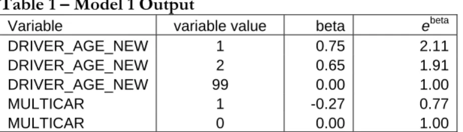
Table 1 – Model 1 Output
Variable variable value beta ebeta
DRIVER_AGE_NEW 1 0.75 2.11
DRIVER_AGE_NEW 2 0.65 1.91
DRIVER_AGE_NEW 99 0.00 1.00
MULTICAR 1 -0.27 0.77
MULTICAR 0 0.00 1.00
In this example, we constrain DRIVER_AGE by letting the offset take on the constrained values for age groups 3 and 4; and the 1.0 for the other age groups. At the same time, we re-code the age group values 3 and 4 to the value 99 to ensure that the model parameters for these levels will be 0. (This is a SAS trick: SAS treats the highest value of a categorical value as the base category.) Therefore, the model estimates “beta” parameters for age groups 1 and 2, as well as the multi-car indicator, subject to the constraint that age groups 3 and 4 must have relativities of 1.05 and 1.25, respectively. The final relativity for each level of DRVER_AGE and MULTICAR will by exp(beta + log_offset) = ebeta*offset. The final rating relativities are displayed below.
Table 2 – Combining Model 1 Parameters with Offset Values
Variable variable value model beta ebeta offset final relativity
DRIVER_AGE 1 0.75 2.11 1 2.11 DRIVER_AGE 2 0.65 1.91 1 1.91 DRIVER_AGE 3 0.00 1.00 1.05 1.05 DRIVER_AGE 4 0.00 1.00 1.25 1.25 MULTICAR 1 -0.27 0.77 1 0.77 MULTICAR 0 0.00 1.00 1 1.00
Construction of a Cross-coverage Tier Score
In many insurance rating plans, a “tier” structure is a rating component that is layered on top of a class plan. In most cases, tier pricing is applied on a policy level across coverages. The purpose of rating tiers is to include in the pricing process further variables – such as personal credit score or not-at-fault accidents – which are not part of standard class plans. Rating tiers can also be used to capture interaction effects between the class plan variables, such as the interaction between driving record and driver age, which are not fully reflected due to the limitation of pricing structures. In the next example we illustrate how an offset technique can be used to create a cross-coverage tier structure.
Suppose we wish to add a tier structure to an existing standard personal auto class plan with two coverages: property damage liability (PD) and comprehensive (Comp). The tiers are to be
comprised of two factors: number of policy-level not-at-fault accidents in the past 3 years (NAF) and credit score (CREDIT). The tier structure and the tier score are required to be the same across the two coverages.
Suppose we start with two separate data files, one for PD liability and one for Comp. Table 3 shows some sample records of the two data files on the exposure/vehicle level. Note that the PD and Comp adjusted exposures were calculated using the logic described in the section of “Exposure Adjustments and Offset”. Specifically, the PD liability adjusted exposure is the unadjusted exposure multiplied by the corresponding territory factors; and the Comp adjusted exposure is the unadjusted exposure multiplied by the corresponding factors for territory, vehicle symbol and deductible.
Table 3
Sample Records from PD Dataset
Policy
Number Number Vehicle
Credit Score Group Policy Level NAF Count Current Plan Rating
Factor Exposure Adjusted Incurred Loss
Adjusted Pure Premium 00003 1 2 1 0.41 0.73 0 0 00004 1 0 0 1.63 1.46 1664 1143 00005 1 0 0 0.58 1.25 0 0 00006 1 2 0 0.61 0.52 0 0 00007 1 1 0 1.12 1.25 1344 1077
Sample Records from Comp Dataset
Policy
Number Number Vehicle
Credit Score Group Policy Level NAF Count Current Plan Rating
Factor Exposure Adjusted Incurred Loss
Adjusted Pure Premium 00003 1 2 1 1.38 1.07 0 0 00004 1 0 0 0.79 1.60 495 309 00005 1 0 0 1.05 1.51 566 375
Our first step is to simply “stack” these two datasets together, adding a coverage indicator to identify whether the record is PD vs. Comp.
Table 4
PD and Comp Combined Dataset
Policy
Number Number Vehicle PD_IND
Credit Score Group Policy Level NAF Count Current Plan Rating
Factor Exposure Adjusted Incurred Loss
Adjusted Pure Premium 00003 1 1 2 1 0.41 0.73 0 0 00004 1 1 0 0 1.63 1.46 1664 1143 00005 1 1 0 0 0.58 1.25 0 0 00006 1 1 2 0 0.61 0.52 0 0 00007 1 1 1 0 1.12 1.25 1344 1077 00003 1 0 2 1 1.38 1.07 0 0 00004 1 0 0 0 0.79 1.60 495 309 00005 1 0 0 0 1.05 1.51 566 375
The following GLM can be used to estimate the parameters for NAF and Credit:
Model 2
Input Dataset: Stacked dataset
Target Variable: Pure Premium (loss / exposure_adj); Predictive Variables: Credit, NAF
Distribution: Tweedie
Link: Log
Offset: PD_Relativity*β1β2··· βp (product of existing rating plan factors)
Weight: exposure_adj;
In the above model specification, we are using the offset to reflect the existing rating plan factors. We must also account for the variation in Pure Premium between the two coverages: clearly we expect a higher Pure Premium for PD records than Comp records. Not including a PD indicator in the model design would lead to a particularly egregious example of omitted variable bias.
In the above model design, we choose to include the PD relativity as an offset factor along with the rating plan factors other than credit score and not-at-fault accident count. Note that other model designs are possible. For example, it would also be possible to include the PD relativity as part of the exposure adjustment step. Either way, we must perform a preliminary analysis to estimate the Pure Premium relativity for PD vs. Comp, and include this relativity either as part of the offset or the exposure adjustment step.
Because our target variable in this example is Pure Premium, the Tweedie is an appropriate choice of distributions. This has been discussed extensively in the actuarial literature [4,6], so we will review this topic only briefly. For claim count (or frequency) modeling, it is customary to assume that the variance of the target variable is proportional to the mean: V(µ)=φµ. This is the “Poisson” model design used in the previous examples. For severity modeling, it is customary to assume that the variance is proportional to the square of the mean: V(µ)=φµ2. This is known as a “Gamma” model design. Pure Premium is the sum of a (Poission distributed) random number of (Gamma distributed) sizes of loss. It is a convenient mathematical fact that the variance of this target variable is proportional to the mean raised to a power between 1 and 2, pє(1,2): V(µ)=φµp. This model
design is also exponential family, and is known as the “Tweedie”.
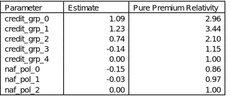
Unfortunately, the commonly used SAS statistical package does not automatically support the Tweedie model in the GENMOD GLM modeling procedure. One alternative to GENMOD is to fit Tweedie models using the NLMIXED procedure. Details of this are given in Appendix C. Table 5 shows the parameter estimates from the above Tweedie model. The PD relativity used in the offset is 3.44.
Table 5 – GLM Outputand Pure Premium Relativities Parameter Estimate Pure Premium Relativity
credit_grp_0 1.09 2.96 credit_grp_1 1.23 3.44 credit_grp_2 0.74 2.10 credit_grp_3 -0.14 1.15 credit_grp_4 0.00 1.00 naf_pol_0 -0.15 0.86 naf_pol_1 -0.03 0.97 naf_pol_2 0.00 1.00
Thus the tier score for a policy with NAF=1 and Credit=2, for example, is exp(0.74 - 0.03)=2.03. Please note that the PD indicator is not used to calculate the tier factor.
Sequential Modeling
The previous two examples, building a credit score and a tiering structure “on top of” an existing rating plan, may be thought of as exercises in “sequential modeling”. By “sequential modeling” we mean building a model to account for variation not already explained by a pre-specified model. The pre-specified model (the existing rating plan in the above examples) in other words serves an as “offset” when building the second model.
Sequential modeling techniques have a wide range of applications. As noted above, the first two examples – estimating rating plan factors after Territory and Symbol factors have been determined in a separate analysis; and building a credit scoring model on top of an existing rating plan – are examples of sequential modeling. Sequential modeling can also be useful for regulatory compliance. For example, California’s Proposition 103 requires that safety/driving record and mileage be the greatest determinants of auto premiums. Insurers typically use sequential methods when developing their rates in California.
We will give one final example of sequential modeling before closing the paper. In this example, we will estimate first the main effects of a rating plan and then an interaction term in sequential fashion. There can be many motivations for sequential modeling strategies such as the one exemplified here. For example, perhaps the interaction factors will be used only in certain states; but the main effect factors are desired to be common across all states. Sequential modeling using an offset would be a practical way to approach such a situation. Another motivation might be that one wishes to keep the main effects model simple, without the complication of estimating an interaction term in the same step.
In this final example, we suppose we are modeling PD pure premium using the three rating variables: driver age group, multicar indicator, and pleasure use indicator. We will build an initial GLM model for these three main effects. We will next build a second model – using the first model score as an offset – to estimate the factors for a driver age/pleasure use interaction term. As discussed above, the “main effects” rating plan might be used nationally; the additional interaction factors might be implemented in selected states.
Model 3
Target Variable: PD Pure Premium (pd loss / pd exposure_adj); Predictive Variables: DRIVER_AGE, MULTICAR, PLEASURE_USAGE
Distribution: Tweedie
Link: Log
Offset: (none)
Weight: exposure_adj;
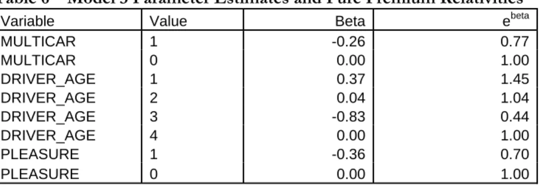
The rating factors resulting from this model are displayed in the table below.
Table 6 – Model 3 Parameter Estimates and Pure Premium Relativities
Variable Value Beta ebeta
MULTICAR 1 -0.26 0.77 MULTICAR 0 0.00 1.00 DRIVER_AGE 1 0.37 1.45 DRIVER_AGE 2 0.04 1.04 DRIVER_AGE 3 -0.83 0.44 DRIVER_AGE 4 0.00 1.00 PLEASURE 1 -0.36 0.70 PLEASURE 0 0.00 1.00
Let η denote the linear component of the scoring formula corresponding to the table above:
η = βDRIVER_AGE + βMULTICAR + βPLEASURE. We will use η as the offset in the model for Step II of the sequence.
Model 4
Target Variable: PD Pure Premium (pd loss / pd exposure_adj); Predictive Variables: DRIVER_AGE * PLEASURE
Distribution: Tweedie
Link: Log
Offset: η
Weight: exposure_adj;
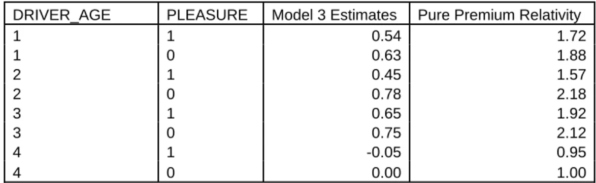
Model 4 differs from Model 3 only in the choice of predictive variables; and the fact that we’re using the linear component of the Model 3 scoring formula (ETA) as the offset. Note although exp(η) is Model 3’s estimate of PD Pure Premium, we are using η, not exp(η), as the offset in Model 4 (below). This is because we are building a multiplicative model (using the log link function). Therefore the offset must be on the log scale.
Table 7 – Model 4 Parameter Estimates and Pure Premium Relativities DRIVER_AGE PLEASURE Model 3 Estimates Pure Premium Relativity
1 1 0.54 1.72 1 0 0.63 1.88 2 1 0.45 1.57 2 0 0.78 2.18 3 1 0.65 1.92 3 0 0.75 2.12 4 1 -0.05 0.95 4 0 0.00 1.00
In states for which Model 4’s interaction factors are not used, the factors in Table 6 constitute the rating plan. In states for which the interaction is intended to be used, we must integrate the results of tables 6 and 7. This is done in tables 8 and 9:
Table 8 – Pure Premium Relativities for Type
Variable Value Relativity
MULTICAR 1 0.77
MULTICAR 0 1.00
Table 9 – Pure Premium Relativities for DRIVER_AGE and PLEASURE PLEASURE
DRIVER AGE PLEASURE=1 PLEASURE=0
1 1.74 2.71
2 1.63 2.26
3 0.71 0.97
4 0.90 1.00
Conclusion
The GLM offset feature is a practical and versatile tool for dealing with a variety of issues such as: data constraints, credibility issues (as in Symbol factor development), regulatory considerations (e.g. California’s Proposition 103), the desire to layer a further rating, scoring, or tier model on top of an existing rating plan (credit scoring, tier factor development), and the need to add state-specific variations to a basic countrywide rating plan (sequential modeling).
Generally speaking, the offset option is helpful when omitted variable bias [OVB] threatens to distort one or more model parameters. The classic use of an offset is to incorporate a measure of exposure when modeling rates. For example if some records in a personal auto dataset correspond to 6-month policies while other records correspond to 12-month policies, then it is appropriate to use (log of) months of exposure as an offset. Failure to do so would raise the specter of OVB: model variables correlated with months of exposure might possibly pick up some of the variation that should be explained by months of exposure. This would result in biased parameter estimates. Beyond this classical use, the offset option is helpful in a number of actuarial applications. For example, we have described how the offset option can be used to build GLM models subject to
certain rating factor constraints; to optimize the rating factors of some, but not all, of the variables in a rating plan; and to build predictive or rating models in sequential fashion. We discussed credit scoring, tier variable creation, and state-exception sub-models as examples of actuarial pricing models built in sequential fashion.
The offset option provides actuaries with a unifying framework – encompassing such traditional techniques as exposure adjustments and loss ratio modeling as an alternative to pure premium modeling – for avoiding omitted variable bias. It is therefore appropriate to consider using an offset when performing a multivariate analysis subject to variable exclusions or other a priori constraints.
References
[1] McClenahan, C. L., “Ratemaking,” Foundations of Casualty Actuarial Science, Casualty Actuarial Society, 1990, 25-90.
[2] Stenmark, A. J., and C. P. Wu, “Simpson’s Paradox, Confounding Variables, and Insurance Ratemaking,”
Proceedings of Casualty Actuarial Society, 2004, Vol. XCI, 133-198
[3] Nelder, John A., and R. W. M. Wedderburn, “Generalized Linear Models,” Journal of the Royal Statistical Society, Series A, 1972, Vol. 135, No. 3, 370-384.
[4] Mildenhall, S. J., “A Systematic Relationship Between Minimum Bias and Generalized Linear Models,”
Proceedings of Casualty Actuarial Society,1999, Vol. LXXXVI, 393-487.
[5] Brockman, M. J., and T. S. Wright, “Statistical Motor Rating: Making Effective Use of Your Data,” Journal of the Institute of Actuaries, 1992, Vol. 119, Part III, 457-526.
[6]Anderson, D., S. Feldblum, C. Modlin, D. Schirmacher, E. Schirmacher, and N. Thandi, "A Practitioner's Guide to Generalized Linear Models", Casualty Actuarial Society Discussion Paper Program, 2004, 1-116.
[7] Fu, L., and C. P. Wu, “Generalized Minimum Biased Models,”Casualty Actuarial Society Forum, Winter 2005, 72-121.
[8] Hilbe, J., Generalized Linear Models and Extensions, College Station, TX: Stata Press, 2001.
[9] Monaghan, J. E., “The Impact of Personal Credit History on Loss Performance in Personal Lines,” Casualty Actuarial Society Forum, Winter 2000, 79-105.
[10] Credit Reports and Insurance Underwriting, NAIC White Paper, 1997, Kansas City, MO: National Association of Insurance Commissioners.
[11] Murphy, K.P., M. J. Brockman, and P. K. W. Lee, “Using Generalized Linear Models to Build Dynamic Pricing Systems,” Casualty Actuarial Society Forum, Winter 2000, 107-139.
[12] Werner, G., and S. Guven, “GLM Basic Modeling: Avoiding Common Pitfalls,” Casualty Actuarial Society
Forum, Winter 2007, 257-272.
[13] Dunn, Peter K., “Occurrence and Quantity of Precipitation can be Modeled Simultaneously,” International Journal of Climatology, 2004, Vol. 24, No. 10, 1234-1239, http://www.sci.usq.edu.au/staff/dunn/research.html [14] Smyth, Gordon K., and Bent Jørgensen, “Fitting Tweedie's Compound Poisson Model to Insurance Claims
Data:Dispersion Modelling,” ASTIN Bulletin, 2002, Vol. 32, No. 1, 143-157,
Appendix A: Two Equivalent Ways of Modeling Frequency with Poisson Regression
Suppose we wish to model claim frequency F as a generalized linear function of several covariates {X1, X2, …, XN}. Let C denote the number of claims for a given policy, and u (for “units”) denote
number of exposures. Then: F=C/u.
We will demonstrate that the following two ways of modeling F are equivalent:
Option 1 Option 2
GLM family: Poisson Poisson
Target: C F
Weight: (none) u
Offset: log(u) (none)
Let us start with Option 1 and demonstrate that it is equivalent to Option 2. Let i denote the observation number. The Poisson regression assumption is that:
! ) ( i c i i i c e c C P i iλ λ − = = Where ) ... ) exp(log( 1 1 2 2 N N i u α β X β X β X λ = + + + + +
Note that if we let:
) ...
exp( 1 1 2 2 N N
i α β X β X β X
μ = + + + +
Then we have the relationship: λi=u*μi.
The log-likelihood function for the Option 1 Poisson regression model is:
κ λ λ λ β α =
∑
−λ )=∑
− + log( )+ ! log( ) , | ( i i i i i c i i c c e c l i i(For simplicity we are assuming that over-dispersion does not exist in the data. That is, φ=1.) We can recast the above expression in terms of F and μ:
) ' ' log( ) ' ) log( ( ) ' ) log( / ( ' ) log( ) log( ) , | ( κ μ κ μ μ κ μ μ κ μ μ κ μ μ β α μi fi i i i i i i i i i i i i i i i i i i i i i i i i i e u f u u c u c u u c u c l −
∑
∑
∑
∑
∑
= + + − = + + − = + + − = + + − =In the above expressions, {κ, κ’, κ’’} denote constants that do not depend on the model parameters. This last expression is the log-likelihood function for the Poisson regression, cast in the terms
Appendix B: Details of the Dataset Used in Examples
The data used in this paper was simulated by Deloitte Consulting using a typical private passenger auto (PPA) rating structure. The data consists of 50,000 vehicle-level records corresponding to 24,993 single-car policies and 11,038 multi-car policies. Two coverages, Property Damage liability (PD) and Comprehensive (Comp), were simulated for each vehicle. By construction, 50% of the vehicles have exposures in both coverages, while the other 50% of the vehicles have PD exposure. The following rating variables were simulated for each vehicle record:
Multicar indicator {0,1} “0” – single car “1” – multi Car
Policy age {0,1,2,…,15}
Driver age group {1,2,3,4}
Pleasure use indicator {0,1} “1” – Pleasure Use “0” – Not Pleasure Use Credit score group {0,1,2,3,4}
Territory {T1, T2, T3, T4}
Vehicle symbol {1,2,3,4,5}
Policy-level at fault accidents {0,1,2+} Policy-level not at fault accidents {0,1,2+}
All of these variables are treated as categorical variables in the examples described in the body of this paper.
The following target fields were also simulated for each vehicle record: PD incurred loss, PD claim count (7,414 claims, or 14%), PD exposure, Comp incurred loss, Comp claim count (6,143 claims, or 12.2%) and Comp exposure.
Appendix C: The Tweedie Compound Poisson Model and Corresponding SAS Code Matthew Flynn, Ph.D.
Following Smyth & Jorgenson [14], section 4.1, page 11, the Tweedie Compound Poisson joint likelihood function as:
(
) (
)
(
)
⎭ ⎬ ⎫ ⎩ ⎨ ⎧ =a n y w p t y p w y n f , ; , , ; , exp ,μ, ϕ ω ϕ ρ ϕ with(
)
(
)
(
p) (
p)
n( )
n y y w p w y n a n α ϕ ϕ αα α Γ ⎭ ⎬ ⎫ ⎩ ⎨ ⎧ − − = + ! 1 2 1 , ; , 1 where α = (2-p)/(p-1) and . 1 2 ( , , ) 1 2 p p t y p y p p μ μ μ = − − − − −.
The SAS codes using “Proc NLMIXED” to fit the above likelihood function for the cross coverage tiering score example in the paper is given as follows:
proc nlmixed data=the_appended_dataset;
parms p=1.5;
bounds 1<p<2;
eta_mu = b0 + c1*(credit_grp=1)+c2*(credit_grp=2)+c3*(credit_grp=3)+c4*(credit_grp=4)
+ naf1*(naf_pol=1)+naf2*(naf_pol=2) + coverage_COMP*(coverage=’COMP’); mu = exp(eta_mu + current_factor); eta_phi = phi0 +
phi_c1*(credit_grp=1)+ phi_c2*(credit_grp=2)+
phi_c3*(credit_grp=3)+ phi_c4*(credit_grp=4)+ phi_naf1*(naf_pol=1)+ phi_naf2*(naf_pol=2) + phi_coverage_COMP*(coverage=’COMP’); phi = exp(eta_phi); n = claims; w = insured; y = pp; t = ((y*mu**(1 - p))/(1 - p)) - ((mu**(2 - p))/(2 - p)); a = (2 - p)/(p - 1); if (n = 0) then loglike = (w/phi)*t; else
loglike = n*((a + 1)*log(w/phi) + a*log(y) - a*log(p - 1) - log(2 - p)) - lgamma(n + 1) - lgamma(n*a) - log(y) + (w/phi)*t;
model y ~ general(loglike); replicate adjexp; estimate 'p' p; run;
(
)
p p y p y t p p − − − = − − 2 1 , , 2 1 μ μ μThe above codes can be broken down into the following major sections:
• First we call the Proc NlMIXED, addressing the desired input dataset:
proc nlmixed data=the_appended_dataset;
The PARMS statement provides a starting value for the algorithm’s parameter search. Multiple starting values are allowed, as well as input from datasets (from prior model runs, for example). With some domain knowledge we anticipate this parameter to be in the neighborhood of 1.5.
parms p=1.5;
Parameters can also be easily restricted to ranges, such as to be positive, and here we require the estimated Tweedie power parameter to fall between one and two.
bounds 1<p<2;
• Next we specify the linear model/predictor for the mean response. Proc NLMIXED does not have the convenient CLASS statement of some of the other regression routines, like Proc GENMOD or Proc LOGISTIC. However, the design matrix can be created “on-the-fly”, so to speak, by effectively including programming statements in the Proc NLMIXED code. Here, we create dummy variables by coding the linear model with logical statements. For example, the phrase, (credit_grp=1) resolves to either true (1) or false (0) at runtime, creating our desired indicator variables to test discrete levels of right-hand side variables. As a reminder, for a GLM, the linear predictor is required to be linear in the estimated parameters, so non-linear effects such as high powers of covariates or splines can be accommodated.
eta_mu = b0 + c1*(credit_grp=1)+c2*(credit_grp=2)+c3*(credit_grp=3)+c4*(credit_grp=4)
+ naf1*(naf_pol=1)+naf2*(naf_pol=2) + coverage_COMP*(coverage=’COMP’);
• Next we create a log link that maps the linear predictor to the mean response. That log link on the left hand side, becomes an exponential as the inverse link (on the right-hand side). mu = exp(eta_mu + current_factor);
• A great feature of using Proc NLMIXED is its flexibility. Here we are specifying what Smyth & Jorgenson [13] refer to as a double GLM. Instead of a single constant dispersion constant, we can fit an entire second linear model with log link for the dispersion factor. eta_phi = phi0 +
phi_c1*(credit_grp=1)+ phi_c2*(credit_grp=2)+ phi_c3*(credit_grp=3)+ phi_c4*(credit_grp=4)+ phi_naf1*(naf_pol=1)+ phi_naf2*(naf_pol=2)
+ phi_coverage_COMP*(coverage=’COMP’);
• Proc NLMIXED allows a number of datastep style programming statements. Here we are assigning input dataset variables claims, insured, and pp as new variables (n, w and y) to be used subsequently in building out our likelihood equation. That way, one can easily adapt pre-existing code to a particular input dataset, without requiring modifications to the “guts” of the log-likelihood equation (it is complicated enough already).
n = claims;
w = insured;
y = pp;
• Now one can begin to specify the loglikelihood. Here, for clarity, we build it out in several steps. Simply refer to the Tweedie Compound Poisson likelihood described above from Smyth & Jorgensen [13], and lay it out.
t = ((y*mu**(1 - p))/(1 - p)) - ((mu**(2 - p))/(2 - p)); a = (2 - p)/(p - 1);
if (n = 0) then
loglike = (w/phi)*t; else
loglike = n*((a + 1)*log(w/phi) + a*log(y) - a*log(p - 1) - log(2
- p)) - lgamma(n + 1) - lgamma(n*a) - log(y) + (w/phi)*t;
Proc NLMIXED includes several pre-specified likelihoods, for example, Poisson and Gamma, the GENERAL specification allows the great flexibility to specify one’s desired model specification.
model y ~ general(loglike);
Weights can either be included directly in the loglikelihood above, or with the handy REPLICATE statement. Each input record in the dataset represents an amount represented by the input variable “adjexp”.
replicate adjexp;
The ESTIMATE statement can easily calculate and report a variety of desired statistics from one’s model estimation. Here, we are interested in the Tweedie Power parameter.
estimate 'p' p;
Without using any of the additional “Mixed” modeling power, Proc NLMIXED performs as a great Maximum Likelihood Estimator using a variety of numeric integration techniques.