Driver Attitudes and Choices: Speed Limits, Seat Belt Use, and Drinking-and-Driving

(1)

Driver Attitudes and Choices:

Speed Limits, Seat Belt Use, and Drinking-and-Driving

Young-Jun Kweon

Associate Research Scientist Virginia Transportation Research Council

Young-Jun.Kweon@VDOT.Virginia.gov Virginia Transportation Research Council

530 Edgemont Road Charlottesville, VA 22903 Phone: 434-293-1949 Fax: 434-293-1990 and Kara M. Kockelman (Corresponding Author)

Associate Professor of Civil, Architectural and Environmental Engineering The University of Texas at Austin kkockelm@mail.utexas.edu

The University of Texas at Austin 6.9 E. Cockrell Jr. Hall Austin, TX 78712-1076

Phone: 512-471-0210 Fax: 512-475-8744

The following paper is a pre-print and the final publication can be found in

Journal of the Transportation Research Forum 45 (3):39-56, 2006.

Presented at the 82nd Annual Meeting of the Transportation Research Board, January 2004

Abstract

A better understanding of attitudes and behavioral principles underlying driving behavior and traffic safety issues can contribute to design and policy solutions, such as, speed limits and seat belt legislation. This work examines the Motor Vehicle Occupant Safety Surveys (MVOSS) data set to illuminate drivers’ seatbelt use, driving speed choices, drinking-and-driving tendencies, along with their attitudes towards speed limits and seat belt laws. Ordered probit, negative binomial, and linear regression models were used for the data analysis, and several interesting results emerged. For example, persons of higher income and with a college education prefer higher speeds, are more likely to use a seat belt, and are more likely to support seat belt laws and/or higher speed limits. However, persons with a college education also tend to drink and drive more often. Pickup drivers are less likely to use seat belts, less likely to support seat belt laws, yet less likely to drink and drive. The number and variety of results feasible with this single data set are instructive as well as intriguing.

Key words Driver attitudes; Driver behavior; Speeding; Motor Vehicle Occupant Safety Surveys (MVOSS)

(2)

INTRODUCTION

Many traffic safety issues have been investigated using crash data such as the General Estimates System (GES), Fatality Analysis Reporting System (FARS), Highway Safety Information System (HSIS), and local police crash records. Conclusions across studies on the impact of speed limit changes (e.g., Chang and Paniati 1990, Wagenaar et al. 1990, and Ledolter and Chan 1996) and the impact of speed variation on traffic safety (e.g., Lave 1985 and 1989, Levy and Asch 1989, Davis 2002, and Kockelman et al. 2006) are not definitive, even with these sophisticated and large datasets. One possible explanation of this discrepancy among studies on the same topic is lack of understanding of road user behaviors and attitudes.

The National Highway Traffic Safety Administration (NHTSA) has conducted the Motor

Vehicle Occupant Safety Surveys (MVOSS) biannually since 1994 by telephone interview. The 2000 MVOSS data include information on driver attitudes towards safety issues (e.g., attitudes towards the current speed limit), driver behaviors (e.g., speed choice and driving frequency), and crash history, as well as on individual and household characteristics (Boyle and Schulman 2001). These are analyzed here.

A better understanding of behavioral principles and circumstances that underlie driving behavior and driver attitudes can enhance various traffic safety policies, including speed limit selection, seat belt legislation, and drunk-driving campaigns. In this regard, the MVOSS data set provides many useful pieces of information for investigation. Knowing who the supporters and opponents of traffic safety-related policies are can be very helpful in crafting and promoting such policies, such as defining target groups for anti-speeding campaigns and driver training programs.

This study investigates several interesting issues relating to these variables. Through these investigations, the study aims to provide behavioral and psychological insights into the U.S. driving population. What follows here is a literature review, model and descriptions, a discussion of results, and conclusions.

LITERATURE REVIEW

A few studies have addressed certain driving behaviors and attitudes using a series of cross-sectional surveys in the U.S. commissioned by Prevention Magazine. Schechtman et al. (1999) attempted to relate drinking habits (frequency and amount) to seat belt use, speed limit obedience, and drunk driving over 11 years. They found no evidence to link drinking habits with seat belt use and speed limit obedience. However, evidence indicated links between frequency and amount of drinking with drunk driving, as expected.

Shinar et al. (1999) used the same datasets as Schechtman et al. (1999) to examine trends in driving behaviors and health maintenance behaviors. They found that the rate of seat belt use increased from 41.5% in 1985 to 74.1% in 1995, along with a slight reduction in drunk driving. The investigators also noted a weak relation between driving behaviors and health maintenance behaviors. Shinar et al. (2001) used more recent Prevention Magazine survey data to investigate associations between seat belt use, speed limit observance, drunk driving, and four demographic characteristics (gender, age, education and income). Their four-way ANOVA models using 1994-1995 data indicated that females reported more law obedience than males in all behavioral categories. Rates of seat belt use increased with age and education level for both males and females. Interestingly, higher education and income levels were associated with speeding. One

(3)

may argue that this is due to higher values of travel time and driving newer vehicles with better safety features, in many cases.

Koushki et al. (1998) reported that Kuwaiti drivers in the same age group, who did not wear seat belts, violated traffic regulations more than twice as often as those who wore seat belts. They also found that seat belt non-users were mostly young and female among Kuwaitis, and their driving behaviors frequently involved changing lanes without signaling and changing travel speed. Their findings confirm that drivers who are reluctant to wear a seat belt tend to be more dangerous drivers and/or take more risks, in general. Regarding crash injury severity, Kim et al. (1995) found seat belt use among Hawaiians contributed significantly to injury reductions and crash survival. He also argued that discouraging alcohol use placed drivers at less risk.

Speed choice also has been investigated. Haglund and Aberg (2000) examined drivers’ attitudes towards speeding and the influence of other drivers on speed choices. Data were collected on Swedish highways, with a speed limit of 90 kilometers per hour (km/h) (56 mph). They concluded that drivers’ decisions regarding speeding are highly correlated with their view of other drivers’ behaviors. Drivers usually overestimated the fraction of high-speed drivers (i.e., those traveling at least 10 km/h over the speed limit); their estimates averaged 50.7%, while the observed percentage was 22.9%. Furthermore, high-speed drivers believed that a high

proportion (58%) of other drivers also qualified as high-speed drivers, indicating a false impression of speed consensus.

Driving speeds are influenced by various factors, including roadway geometry, driver attitudes and environmental factors (e.g., weather and enforcement). Kanellaidis et al. (1990) studied passenger car speeds on horizontal curves of two-lane rural roads in Greece. A total of 207 Greek drivers rated the impact of 14 elements of the road’s environment (e.g., sight distance, pavement condition, and lane width) on their choice of speed. Drivers who tended to violate speed limits rated all types of signage (e.g., warning signs) significantly lower than speed limit observers. Speed limit offenders also paid less attention to roadway design.

Liang et al. (1998) found considerable reductions in mean speed and significant increases in speed variance under foggy and snowy conditions on Interstate 84 in Idaho, while Edwards (1999) only reported small reductions in both mean and variance under rainy and foggy conditions on the M4 Motorway in the U.K. Vaa (1997) found statistically significant and somewhat large reductions in average speeds and fraction of speeders due to increased police enforcement on Norway highways. Kockelman et al. (2006) found average speed increases in cross-section to be double those in before/after studies of speed-limit increases, and modeled optimal speed choices as a trade-off of crash, speed limit violation, and delay costs. They also found instantaneous speed variations (across individual vehicles) to hardly depend on speed limits and roadway design attributes, and they concluded that higher speed limits have their greatest effect on crash outcomes, in terms of injury severity.

Many behaviors are recorded as discrete responses (e.g., yes/no) in data sets. Discrete-response models are now common in assessing crash results. For example, Kockelman and Kweon (2002) applied an ordered probit model for prediction of driver injury severity using the 1998 GES data and developed separate models for single-vehicle, two-vehicle and multi-vehicle crashes. As expected, higher travel speeds were predicted to significantly increase injury severity. Females and older persons were also predicted to be at greater risk for severe injury, if they experience a

(4)

crash as a driver. Their results are similar to those of O’Donnell and Connor (1996), who used Australian crash records and ordered logit and probit models. They found that driving light-duty trucks at high speeds, not wearing seat belts, and head-on collisions all increased the likelihood of severe injury and fatality.

Cooper (1997) used binary logit models to investigate the relationship between various violation convictions (e.g., exceeding the speed limit and disobeying signals) and crash involvement based on data for British Columbia, Canada. In order to reduce serious and fatal crashes, he concluded that the focus should be on excessive speeders (40 km/h or more over the speed limit). Simply exceeding the speed limit, while statistically significant, was not a primary predictor of increased risk of serious injury. Many others have modeled crash counts (e.g., Miaou 1994, Kim et al. 1995; Gebers 1998, and Ivan et al. 1999) using Poisson and negative binomial models. The negative binomial model is typically more appropriate than the Poisson, since it allows for unobserved heterogeneity while permitting over-dispersion in the data (rather than requiring that variance equal mean). Thus, it was used here to examine the frequency of drinking and driving. MODELS

Three different model specifications were used. Brief general descriptions of two models – ordered probit and negative binomial models – are provided here. Standard ordinary least squares (OLS) regression also was performed, but is not described here.

Ordered Probit Model

In an ordered probit model, the focus is on the probability of one of many possible, ordered responses: (1) y∗_i =β′x_i +ε_i, where ε_i ~ N(0,1) (2) = if 1 ≤ = ′ ≤ , for =0 to −1 ∗ − y m J m yi τm i βxi τm

where y_i∗ is the latent and continuous underlying measure of response, yi is the observed and

coded discrete measure of response, xi denotes a set of explanatory variables, β denotes a set of

coefficient parameters (to be estimated), τm denote threshold parameters (to be estimated, where

−∞ = −1

τ and τ_J₋₁ =∞), m is the observed coded discrete response and J is the number of response levels or categories. Figure 1 presents the correspondence between latent continuous response levels,y_i∗, and the observed discrete response levels, yi.

Figure 1: Relationship Between Latent and Observed Responses

yi 0 1 2 ··· J-2 J-1 τ-1 =−∞ τ0 τ1 τ2 ··· τJ−3 τJ−2 τJ-1=−∞ ∗ i y

For example, y_i= 0 if an individual i thinks current speed limits are too low, 1 if these are about right, and 2 if they are felt to be too high. Here, J = 3. The associated probabilities are as follows:

(5)

(3) ⎪⎩ ⎪ ⎨ ⎧ ′ − Φ − = − = − = ′ − Φ − ′ − Φ = = ′ − Φ = = = − − ) ( 1 ) 1 Pr( ) 2 , , 1 ( if ) ( ) ( ) Pr( ) ( ) 0 Pr( 2 1 0 i J i i i m i m i i i i J y J m y m y y p x β x β x β x β τ τ τ τ K

where Φ(⋅)denotes the standard normal cumulative distribution function. The product of these probabilities is the likelihood function, which assumes independent responses across individuals

in the sample:

∏

= = n i i p L 1 ) , | , (β τ y X .

Negative Binomial Model

Count data are non-negative, integer values. These characteristics often render linear regression models inappropriate, while making Poisson models a popular alternative (with an exponential function of explanatory variables for the rate term, λ).

Poisson models do not allow for unobserved heterogeneity and presume equidispersion (such that mean equals variance). A negative binomial model adds a random disturbance (ε_i) to the rate function of the Poisson model as follows:

(4) μi =exp(β′xi+εi)=λiδi

where μi= expected value of observational unit i’s count (yi), )λi =exp(β′xi , and δi =exp(εi).

Assumption of a gamma distribution for δ_i results in a negative binomial probability mass function (PMF), as follows: (5) ! ) )( exp( ! ) exp( ) Pr( i y i i i i i y i i i y y y i i λδ λδ μ μ − = −

= and exp( )for 0

) ( ) ( 1 > Γ = − i i i v i i v i i v v v v g i i δ δ δ where y_i= 0, 1, 2,…, y_i!=

∏

y₌i

k 1k (e.g., 3!=1×2×3), )g(δi = a gamma probability density function (PDF) with a single parameter vi =α−1 (α >0), and

2 )

|

(yi i i i

Var x =μ +αμ ; so that α is the distribution’s over-dispersion parameter.

In cases where α =0, the negative binomial reduces to a Poisson distribution. As an example application of this model based on the MVOSS data, one can analyze the number of days that a respondent reports having imbibed alcohol and driven in the past 30 days. Readers may consult Cameron and Trivedi (1986) for details on the negative binomial model.

DATA

The 2000 Motor Vehicle Occupant Safety Survey (MVOSS) data were collected between

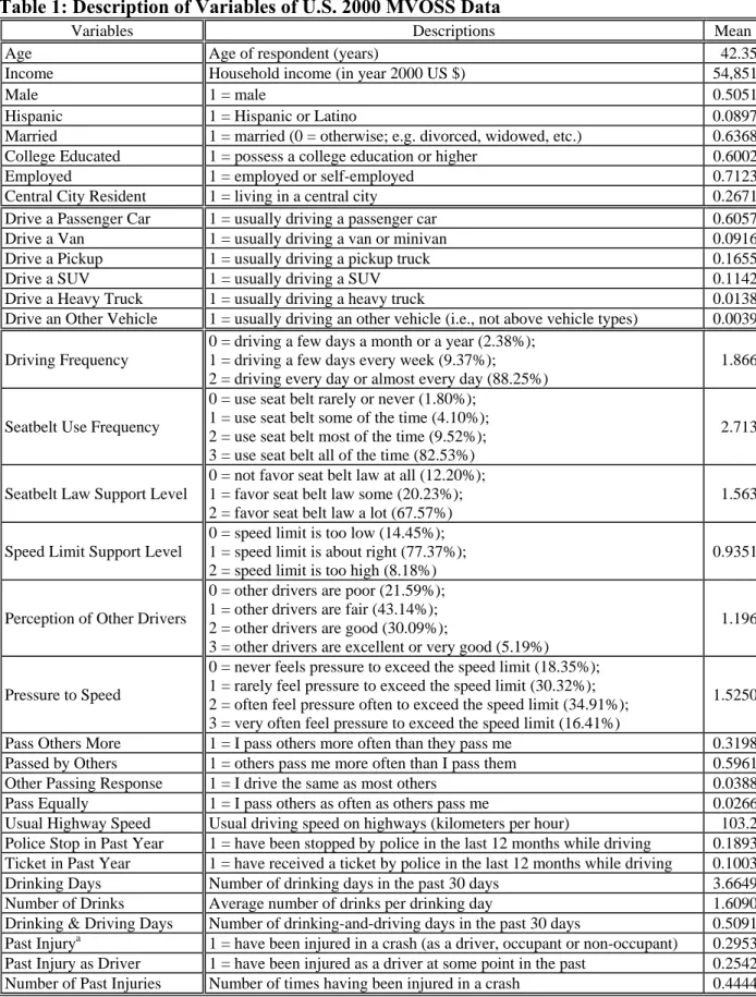
November 2000 and January 2001. Data were obtained from 6,072 respondents, age 16 or older, residing in all 50 U.S. states and Washington, D.C. The survey emphasized traffic safety issues, including driving frequency, seat belt use, and driving attitudes. Basic variable details are shown in Table 1. Due to non-response on certain questions, the sample sizes in the final analyses vary from 4,057 to 4,137, depending on which explanatory variables were used. Household income, originally a categorical variable, was made continuous by using approximate median values in each category.

(6)

Table 1: Description of Variables of U.S. 2000 MVOSS Data

Variables Descriptions Mean

Age Age of respondent (years) 42.35

Income Household income (in year 2000 US $) 54,851

Male 1 = male 0.5051

Hispanic 1 = Hispanic or Latino 0.0897

Married 1 = married (0 = otherwise; e.g. divorced, widowed, etc.) 0.6368

College Educated 1 = possess a college education or higher 0.6002

Employed 1 = employed or self-employed 0.7123

Central City Resident 1 = living in a central city 0.2671

Drive a Passenger Car 1 = usually driving a passenger car 0.6057

Drive a Van 1 = usually driving a van or minivan 0.0916

Drive a Pickup 1 = usually driving a pickup truck 0.1655

Drive a SUV 1 = usually driving a SUV 0.1142

Drive a Heavy Truck 1 = usually driving a heavy truck 0.0138

Drive an Other Vehicle 1 = usually driving an other vehicle (i.e., not above vehicle types) 0.0039 Driving Frequency

0 = driving a few days a month or a year (2.38%); 1 = driving a few days every week (9.37%); 2 = driving every day or almost every day (88.25%)

1.866

Seatbelt Use Frequency

0 = use seat belt rarely or never (1.80%); 1 = use seat belt some of the time (4.10%); 2 = use seat belt most of the time (9.52%); 3 = use seat belt all of the time (82.53%)

2.713

Seatbelt Law Support Level

0 = not favor seat belt law at all (12.20%); 1 = favor seat belt law some (20.23%); 2 = favor seat belt law a lot (67.57%)

1.563

Speed Limit Support Level

0 = speed limit is too low (14.45%); 1 = speed limit is about right (77.37%); 2 = speed limit is too high (8.18%)

0.9351

Perception of Other Drivers

0 = other drivers are poor (21.59%); 1 = other drivers are fair (43.14%); 2 = other drivers are good (30.09%);

3 = other drivers are excellent or very good (5.19%)

1.196

Pressure to Speed

0 = never feels pressure to exceed the speed limit (18.35%); 1 = rarely feel pressure to exceed the speed limit (30.32%); 2 = often feel pressure often to exceed the speed limit (34.91%); 3 = very often feel pressure to exceed the speed limit (16.41%)

1.5250

Pass Others More 1 = I pass others more often than they pass me 0.3198

Passed by Others 1 = others pass me more often than I pass them 0.5961

Other Passing Response 1 = I drive the same as most others 0.0388

Pass Equally 1 = I pass others as often as others pass me 0.0266

Usual Highway Speed Usual driving speed on highways (kilometers per hour) 103.2 Police Stop in Past Year 1 = have been stopped by police in the last 12 months while driving 0.1893 Ticket in Past Year 1 = have received a ticket by police in the last 12 months while driving 0.1003

Drinking Days Number of drinking days in the past 30 days 3.6649

Number of Drinks Average number of drinks per drinking day 1.6090

Drinking & Driving Days Number of drinking-and-driving days in the past 30 days 0.5091 Past Injurya 1 = have been injured in a crash (as a driver, occupant or non-occupant) 0.2953 Past Injury as Driver 1 = have been injured as a driver at some point in the past 0.2542 Number of Past Injuries Number of times having been injured in a crash 0.4444

a

(7)

Among the variables in the MVOSS data relating to traffic safety, those that merit special examination are seat belt usage, response to speed limits and seat belt laws, preferred driving speed, and drinking and driving. The relationship between these variables and a set of

explanatory variables – including traffic crash history, individual characteristics (e.g., age and education level), recent drinking habits (e.g., drinking frequency and amount), vehicle type, and employment – was investigated. Separate analyses were carried out for each variable of interest, using a discrete choice model (ordered probit), a count data model (negative binomial), and a linear regression model (for speed choice).

It should be mentioned that several of these MVOSS variables involve stated preferences (e.g., support for seat belt laws) and sensitive stated behaviors (e.g., drinking days per month and speed choice). Respondents may not know their true response or may choose to “color” their response to hide the truth. (Readers may be interested in Corbett’s (2001) and Bradburn and Sudman’s (1979) discussions of these issues, as well as survey design.) Such tendencies certainly can bias results (e.g., biasing estimates of drinking and driving to the low side and support for seat belt laws to the high side). For example, 82.5% of MVOSS respondents reported using the shoulder belt all of the time, and 9.5% reported using their belt most of the time. In contrast, the National Occupant Protection Use Survey (NOPUS) data, collected at 2,063 sites in October and November of 2000, suggest that only 55% to 74% of adults (across different vehicle types) wear shoulder belts (NHTSA 2001). Therefore, there is probably some over-reporting of seat belt use in the MVOSS data.

RESULTS AND DISCUSSIONS

Model outputs are provided in Tables 2 through 6. In each of these, an initial model including all possible explanatory variables of interest, as shown in Table 1 was estimated, and a final model was then developed, to recognize only those variables that remained statistically significant at the 10% level (p-value ≤ 0.10), after a series of step-wise deletions. Only the final model outputs are presented here. Ordered probit and negative binomial models were estimated using maximum likelihood (ML) estimation techniques, and a linear model was estimated using OLS.

Along with estimates of coefficients (and thresholds for an ordered probit model), a likelihood ratio index (LRI) or McFadden’s pseudo R2, is provided for MLE models, which represents the ratio of likelihood values of models estimated with and without explanatory variables.1 All model estimations were performed using LIMDEP 7.0.

Perceptions of Current Speed Limits

A total of 76.6% of the survey respondents reported being “satisfied” with current speed limits, 16.2 % felt they were too low, and 7.2% thought they were too high. As a point of comparison, Haglund and Aberg (2000) reported figures of 61.1%, 37.0%, and 1.9%, respectively, for Swedes on highways with a 90 km/h (56 mph) speed limit. Of course, the MVOSS survey of American drivers asked a more general question, and U.S. freeway speeds are often above 100 km/h. Thus, it is not unusual to expect that Americans may be less likely to want higher limits than their Swedish counterparts.

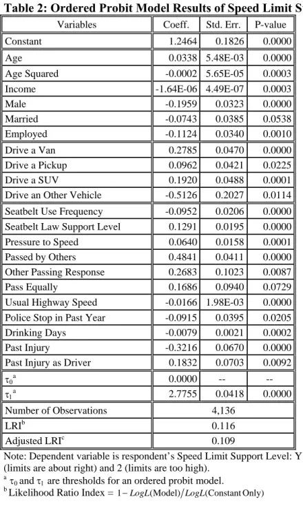
The perceptions on the current speed limits were analyzed using the ordered probit model, and Table 2 shows these results. Positive signs on estimated coefficients suggest that respondents are more likely to consider current speed limits to be too high, and thus favor lowered limits.

(8)

Conversely, negative signs on coefficients indicate that respondents are less likely to consider current speed limits to be too high, and thus favor higher limits.

According to Table 2, males, employed, married, and higher-income drivers tend to favor higher speed limits, in contrast to drivers of light-duty-trucks including pickup trucks, vans and sport-utility vehicles (SUVs) that favor lower speed limits. People who favor seat belt laws, those who are pressured to speed up by other drivers, and those who have experienced injury crashes as drivers tend to support lowering speed limits. In contrast, less frequent seatbelt users, those who frequently pass others on the highway (the reference group for all passing responses), those who have recently been stopped by a police officer, those who drink more often, and/or those who indicated higher driving speeds tend to favor speed limit increases

Table 2: Ordered Probit Model Results of Speed Limit Supports

Variables Coeff. Std. Err. P-value

Constant 1.2464 0.1826 0.0000

Age 0.0338 5.48E-03 0.0000

Age Squared -0.0002 5.65E-05 0.0003

Income -1.64E-06 4.49E-07 0.0003

Male -0.1959 0.0323 0.0000 Married -0.0743 0.0385 0.0538 Employed -0.1124 0.0340 0.0010 Drive a Van 0.2785 0.0470 0.0000 Drive a Pickup 0.0962 0.0421 0.0225 Drive a SUV 0.1920 0.0488 0.0001

Drive an Other Vehicle -0.5126 0.2027 0.0114 Seatbelt Use Frequency -0.0952 0.0206 0.0000 Seatbelt Law Support Level 0.1291 0.0195 0.0000

Pressure to Speed 0.0640 0.0158 0.0001

Passed by Others 0.4841 0.0411 0.0000

Other Passing Response 0.2683 0.1023 0.0087

Pass Equally 0.1686 0.0940 0.0729

Usual Highway Speed -0.0166 1.98E-03 0.0000

Police Stop in Past Year -0.0915 0.0395 0.0205

Drinking Days -0.0079 0.0021 0.0002

Past Injury -0.3216 0.0670 0.0000

Past Injury as Driver 0.1832 0.0703 0.0092

τ0a 0.0000 -- --

τ1a 2.7755 0.0418 0.0000

Number of Observations 4,136

LRIb 0.116

Adjusted LRIc 0.109

Note: Dependent variable is respondent’s Speed Limit Support Level: Y = 0 (current speed limits are too low), 1 (limits are about right) and 2 (limits are too high).

a_τ

0 and τ1 are thresholds for an ordered probit model.

b

(9)

c

Adjusted Likelihood Ratio Index = 1−(LogL(Model)−k) LogL(ConstantOnly), where k is the number of estimated parameters.

Figure 2 illustrates some of the model’s predictions. In order to create this figure, the values for indicators for married and employed were set to one (as a reference individual) and average values of all other explanatory variables were used in the probability function of the ordered probit model (Equation 3 with J=3), Pr(y_i =2)=1−Φ(τˆ₁−βˆ′x_i) whereτˆ₁ and βˆ are provided in Table 2. Then, the values for age, indicators for gender and vehicle types were varied. Figures 3 through 6 were created in a similar way.

Older persons are predicted to respond that current speed limits are too high; however, this trend tops out at about age 80. The gender effect is much greater than the vehicle-type effect: females are more likely to consider current speed limits to be too high, regardless of the vehicle types that they use. As alluded to above, van drivers are estimated to be most likely to favor lowered limits, SUV drivers follow, pickup truck drivers are next, and passenger car drivers (the reference group for the vehicle type indicator variables) are least likely to support lowered speed limits. These are findings for the reference person who is married and employed and has average conditions for all other factors (e.g., has drunk alcohol on 3.6 “occasions” [days] during the past month).

Figure 2: Probability of Considering the Current Speed Limit to be Too High

0.00 0.02 0.04 0.06 0.08 0.10 0.12 0.14 0.16 0.18 0.20 10 20 30 40 50 60 70 80 90 100 Age (years) P robabilit y ( C ur rent S p e ed Lim it is T

oo High) female driving minivans

female driving SUVs

female driving pickups

female driving passenger cars and male driving SUVs male driving minivans

male driving pickups

male driving passenger cars

Note: (1) Reference individual is married and employed, and exhibits average values of all other explanatory variables included in Table 2. (2) The curves for females driving passenger cars and males driving SUVs are too close to one another to distinguish visually; thus, they are presented as a single curve.

Speed Choices on Highways

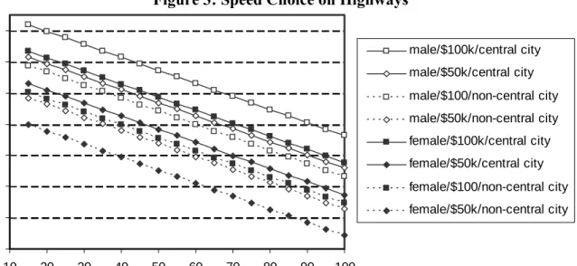
Table 3 and Figure 3 show the OLS model results for predictions of driver speed choices on highways. Respondents’ reports of their usual highway speeds tend to increase with their household income, alcohol consumption (amount and frequency), and recent traffic violations. Male, younger, college-educated persons, frequent drivers, those living in central cities, and those who have been recently stopped or cited by police also tend to prefer higher speeds. Based on this finding, public anti-speeding campaigns should target such drivers. Those who are older,

(10)

employed, Hispanic, drive SUVs, and regard others as “good” drivers prefer lower speeds. The potential reason why drivers with higher household income tend to drive faster and support higher speed limits might be that they value their travel time more highly – and drive more expensive vehicles with better acceleration and safety features.

Table 3: Linear Regression Model Results of Speed Choice on Highways

Constant 63.3613 0.7546 0.0000

Age -0.0419 7.84E-03 0.0000

Income 5.20E-05 1.23E-05 0.0000

Income Squared -2.09E-10 8.21E-11 0.0109

Male 0.8541 0.2198 0.0001

Hispanic -0.7340 0.3752 0.0504

College Educated 1.1627 0.2288 0.0000

Employed -0.7075 0.2589 0.0063

Central City Resident 1.3134 0.2405 0.0000

Drive a SUV -1.8567 0.6620 0.0050

Driving Frequency 1.4622 0.2775 0.0000

Perception of Other Drivers -1.3743 0.2369 0.0000

Passed by Others 0.3594 0.1123 0.0014

Other Passing Response -4.5226 0.2515 0.0000

Pass Equally -2.5151 0.5635 0.0000

Police Stop in Past Year 0.9598 0.3773 0.0110

Ticket in Past Year 0.8827 0.4855 0.0690

Drinking Days 0.0328 0.0175 0.0604

Number of Drinks 0.2881 0.0648 0.0000

Number of Observations 4,136

R-squared 0.226

(11)

Figure 3: Speed Choice on Highways 64 65 66 67 68 69 70 71 10 20 30 40 50 60 70 80 90 100 Age (years) S peed on H ig h w a y s ( m ph) male/$100k/central city male/$50k/central city male/$100/non-central city male/$50k/non-central city female/$100k/central city female/$50k/central city female/$100/non-central city female/$50k/non-central city

Notes: (1) Reference individual is an employed, non-Hispanic, married person with a college degree, and exhibits average values of all other explanatory variables included in Table 3. (2) $50k denotes an annual household income of $50,000.

Seat Belt Use

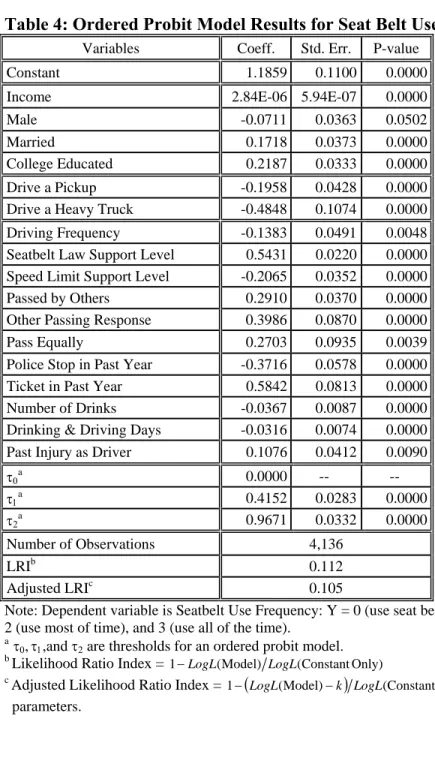
Wearing a seat belt plays a crucial role in diminishing the severity of crashes for vehicle occupants (Kim et al. 1995, NHTSA 2004, and Shults et al. 2004). Table 4 displays the results of an ordered probit model for frequency of seat belt use while driving. The positive signs of the coefficients are interpreted in the same way as in Table 2: as the associated explanatory

variable’s value increases, respondents are more likely to wear their seat belts more often. A negative sign means that as the particular independent variable increases, respondents are less likely to wear their seat belts more often. Figure 4 illustrates how model estimates of

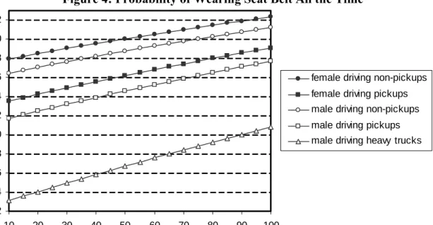
individuals’ probabilities of responding that they “always wear their seat belt” vary with age, gender, and vehicle type (pickup truck, heavy-duty truck, and any other vehicle).

Using an ordered probit model for driver-reported frequency of seat belt use, greater belt use is expected to occur among married, college-educated women, and having higher household incomes (as well as among those who favor a seat belt law). However, as shown in Figure 4, the effect of certain vehicle types was estimated to dominate that of gender. Thus, male passenger car drivers are estimated to be more likely to always use their seatbelts than pickup-driving females (when they are married and college-educated). In addition to males and pickup or heavy-truck drivers, more frequent drivers, those recently stopped by police, those more likely to pass other vehicles (the reference group for passing responses), more frequent imbibers of alcohol, and those drinking and driving more frequently are estimated to be less likely to wear a seat belt (Table 4).

However, those having received a traffic violation in the past 12 months along with those who favor higher speed limits, and have been injured as a driver are more likely to use seat belts often. In general, Shinar et al.’s (2001) seatbelt-use findings relating to education levels are consistent with ours; however, they estimate that the positive income effect applies only to females using Prevention Magazine’s survey data from 1983 through 1995.

(12)

Table 4: Ordered Probit Model Results for Seat Belt Use

Constant 1.1859 0.1100 0.0000

Income 2.84E-06 5.94E-07 0.0000

Male -0.0711 0.0363 0.0502

Married 0.1718 0.0373 0.0000

Drive a Pickup -0.1958 0.0428 0.0000

Drive a Heavy Truck -0.4848 0.1074 0.0000

Driving Frequency -0.1383 0.0491 0.0048

Seatbelt Law Support Level 0.5431 0.0220 0.0000 Speed Limit Support Level -0.2065 0.0352 0.0000

Passed by Others 0.2910 0.0370 0.0000

Other Passing Response 0.3986 0.0870 0.0000

Pass Equally 0.2703 0.0935 0.0039

Police Stop in Past Year -0.3716 0.0578 0.0000

Ticket in Past Year 0.5842 0.0813 0.0000

Number of Drinks -0.0367 0.0087 0.0000

Drinking & Driving Days -0.0316 0.0074 0.0000

Past Injury as Driver 0.1076 0.0412 0.0090

τ0a 0.0000 -- -- τ1a 0.4152 0.0283 0.0000 τ2a 0.9671 0.0332 0.0000 Number of Observations 4,136 LRIb 0.112 Adjusted LRIc 0.105

Note: Dependent variable is Seatbelt Use Frequency: Y = 0 (use seat belt rarely or never), 1 (use some of the time), 2 (use most of time), and 3 (use all of the time).

a_τ

0,τ1,and τ2 are thresholds for an ordered probit model. b

Likelihood Ratio Index = 1−LogL(Model) LogL(ConstantOnly)

c

(13)

Figure 4: Probability of Wearing Seat Belt All the Time 0.72 0.74 0.76 0.78 0.80 0.82 0.84 0.86 0.88 0.90 0.92 10 20 30 40 50 60 70 80 90 100 Household Income ($1000) P ro b a b ilit y ( A lw a y s U s e S e a t B e lt )

female driving non-pickups female driving pickups male driving non-pickups male driving pickups male driving heavy trucks

Notes: (1) Reference individual is married and college-educated, and exhibits average values of all other

explanatory variables included in the model of Table 4. (2) Non-pickups mean any vehicles other than pickups and trucks.

Support for Seat Belt Laws

Respondents’ support for seat belt laws also was estimated via an ordered probit specification, and the results are presented in Table 5 and Figure 5. The positive signs of the coefficients in Table 5 are interpreted in the same way as in Tables 2 and 3: as the values of the variables increase, respondents are more likely to support seat belt laws. According to Table 5, males, pickup, SUV and heavy truck drivers, those with less income and/or education, those who drive and/or use a seat belt less frequently, and those with recent traffic violations are less likely to support a seat belt law. Those who prefer higher speed limits, choose higher speeds and/or drink more are predicted to be less likely to favor a seat belt law, while married persons, Hispanic, those who view others as “good drivers”, those who reside in central cities, and those who feel pressured to speed up by other drivers showed more support for such a law.

(14)

Table 5: Ordered Probit Model Results for Support of Seat Belt Laws

Constant 0.5614 0.1939 0.0038

Age -0.0217 5.30E-03 0.0000

Age Squared 0.0002 5.27E-05 0.0000

Income Squared 1.04E-11 3.14E-12 0.0010

Male -0.3713 0.0311 0.0000

Hispanic 0.3417 0.0502 0.0000

Married 0.0813 0.0350 0.0202

Central City Resident 0.2518 0.0368 0.0000

Drive a Pickup -0.1843 0.0380 0.0000

Drive a SUV -0.0768 0.0458 0.0935

Seatbelt Use Frequency 0.4370 0.0186 0.0000

Speed Limit Support Level 0.1928 0.0288 0.0000 Perception of Other Drivers 0.0472 0.0162 0.0036

Pressure to Speed 0.0391 0.0148 0.0080

Passed by Others 0.0577 0.0341 0.0904

Pass Equally -0.3487 0.0776 0.0000

Usual Highway Speed -0.0052 0.0021 0.0122

Ticket in Past Year -0.1469 0.0501 0.0034

Number of Drinks -0.0409 0.0079 0.0000 Past Injury -0.1064 0.0311 0.0006 τ0a 0.0000 -- -- τ1a 0.8162 0.0241 0.0000 Number of Observations 4,136 LRIb 0.101 Adjusted LRIc 0.094

Note: Dependent variable is Seatbelt Law Support Level: Y = 0 (Not in favor seat of belt law at all), 1 (favor seat belt law somewhat) and 2 (favor seat belt law a lot).

a _τ

0 and τ1 are thresholds for an ordered probit model. b

c

(15)

As illustrated in Figure 5, the gender effect exceeds the vehicle-type effect, and females are predicted to be more likely to favor seat belt laws, irrespective of vehicle type. In addition, support for seat belt laws varies in a convex way with age: declining with age up to age 50, and then increasing.

Figure 5: Probability of Strongly Favoring Seat Belt Laws . 0.35 0.40 0.45 0.50 0.55 0.60 0.65 0.70 0.75 10 20 30 40 50 60 70 80 90 100 Age (years) P ro babi lit y ( F av o r S eat B e lt Law )

female driving passenger cars female driving SUVs

female driving pickups male driving passenger cars male driving SUVs

male driving pickups

Notes: Reference individual is non-Hispanic, married, and college-educated, and exhibits average values of all other explanatory variables included in Table 5’s model

Drinking and Driving

Drinking and driving (during the past 30 days) was examined using a negative binomial regression model, and the results are displayed in Table 6 and Figure 6. Positive signs of

coefficients in Table 6 suggest that, as the values of the associated explanatory variables increase, respondents are more likely to have imbibed alcohol and then driven in the past 30 days.

Negative signs have the opposite interpretation. In estimating the number of days one had been recently drinking and driving, it was found that the number of drinks per event had almost twice the effect of the number of drinking days in the past month. Male, employed persons, college-educated persons, and those recently stopped by police reported more drinking and driving. More frequent driving was associated with more drinking and driving, as one may expect. Married people and those who more often wear seat belts were less likely to drink and drive. Those who drive pickups or heavy trucks were less likely to drink and drive than those driving other types of vehicles.

(16)

Table 6: Negative Binomial Model Results of the Frequency of Drinking and Driving

Constant -5.1852 0.5522 0.0000

Age 0.0489 0.0197 0.0000

Age Squared -0.0004 2.07E-04 0.0664

Male 0.7699 0.1125 0.0000

Married -0.4285 0.1173 0.0003

Employed 0.3303 0.1479 0.0255

Drive a Pickup -0.2804 0.1410 0.0467

Seatbelt Use Frequency -0.1766 0.0824 0.0322

Passed by Others -0.3386 0.1092 0.0019

Police Stop in Past Year 0.2212 0.1267 0.0808

Drinking Days 0.1460 0.0096 0.0000 Number of Drinks 0.2666 0.0450 0.0000 αa _4.1502 _0.2881 _0.0000 Number of Observations 4,137 LRIb 0.347 Adjusted LRIc 0.343

Note: Dependent variable is Drinking & Driving Days: Y = the number of days of drinking and driving in the past 30 days.

a _α

is the overdispersion parameter: _Var₍_Y_|_X₎₌_μ₊_αμ2_. b

c

(17)

Figure 6: Frequency of Drinking and Driving in the Past 30 Days 0 0.1 0.2 0.3 0.4 0.5 10 20 30 40 50 60 70 80 90 100 Age (years) N u m b e r of D ri n k ing and D ri v ing D a y s .

Male driving non-pickups Male driving pickups Female driving non-pickups Female driving pickups

Notes: Reference individual is married, employed, and college-educated, and exhibits average values of all other explanatory variables included in the model of Table 6.

Figure 6 presents the effects of age, gender and vehicle types on the number of drinking and driving days in the past 30 days. Males and those driving non-pickup trucks including passenger cars, SUVs, and vans are more likely to drink and drive with higher frequency than females and those driving pickup trucks. However, the gender effect is much greater than the vehicle-type effect. As a driver ages, the number of drinking and driving days tends to increase, until around age 65.

CONCLUSIONS

This work relies largely on discrete-response (ordered probit) models and count data (negative binomial) models for analysis of the MVOSS. A standard linear regression model also was used to estimate usual highway speed choice. Dependent variables included seat belt use, frequency of drinking and driving, attitudes toward speed limits and a seat belt law, and speed choices on highways in the U.S.

There are a multitude of results available from this work. For example, males are less likely to use a seat belt and favor seat belt laws, but more likely to favor raised speed limits, to drive faster on highways, and to drive after drinking. In general, males are found to exhibit riskier behaviors and less favorable attitudes towards safety policies than females.

Younger persons tend to prefer higher speed limits and choose higher driving speeds on highways. Persons around age 50 are estimated to be among those least likely to support seat belt laws; and those near 85 years of age are most likely to consider speed limits to be too high, and therefore are most likely to support a reduction of speed limits. Interestingly, there is relatively little spread in reported speed preferences: the “average” respondent at the age of 20 prefers to travel 70 mph on highways, but 67 mph at the age of 75.

(18)

With regard to vehicle types, those who drive pickups and heavy trucks are less likely to use a seat belt, less likely to favor seat belt laws, and less likely to drive after drinking. Drivers of vans, SUVs, and pickups are more likely to support lowering the speed limits than passenger car drivers.

Higher household incomes and educational attainment increase the predicted probabilities of seat belt use and one’s support of seat belt laws; however, higher-income drivers tend to support higher speed limits, and those with a college education appear to drink and drive more often. High income and college-educated drivers may value their lives and time more (and drive more expensive vehicles with more safety features and better acceleration performance), but the college educated also appear to value their alcohol consumption more (thus driving after drinking).

This summary relates just a few of the results quantified in the model outputs presented here. It is hoped that these will be useful to policymakers and traffic engineers in the domain of traffic safety for the traveling public. Anticipating public reaction to drunk-driving campaigns, speed limits, and seat belt regulations is important and useful. For example, efforts to reduce drunk driving may find it useful to focus on drivers who are young, male, employed, and college-educated (or about to become college college-educated). To boost seat belt usage rates, it may be more effective to target males driving pickups and heavy-duty trucks. Moreover, policymakers and public information officers in states seeking to enact more stringent seat belt laws (e.g., shifting from secondary to primary enforcement laws)2 may do well to seek support among those who are middle-aged, male, without a college degree, of lower income, and driving pickups, SUVs, or trucks. Targeted messages on safe driving practices can make a difference – saving lives, time, money and other resources. An understanding of human behavior on the roadway is a valuable step in this direction.

ACKNOWLEDGEMENTS

We are grateful to Alan Block in the Office of Research and Traffic Records of the National Highway Traffic Safety Administration for providing us with the MVOSS data set, and to several anonymous referees for their valuable suggestions. We thank Annette Perrone for her excellent editorial assistance and the National Cooperative Highway Research Program (NCHRP) for sponsoring the study (under contract number 17-23).

Endnotes

1

Low LRI (e.g., 0.1) is very common in many discrete-response models of human behaviors and traffic safety. For example, see Graham et al. (2005), Katila et al. (2004), and Noland and Oh (2004). In the field of traffic safety research, interpretation of statistically significant relationships is felt to be far more important than goodness of fit.

2

A primary enforcement law permits the police to stop the vehicle when it observes the seat belt violation, while a secondary law permits the police to issue a citation only after it stops the vehicle for another violation and observes the seat belt violation.

(19)

REFERENCES

Boyle, J. M. and P. V. Schulman. 2000 Motor Vehicle Occupant Survey, Vol. 1 Methodology

Report (DOT HS 809 388). National Highway Traffic Safety Administration (NHTSA),

Washington, D.C., 2001.

Bradburn, N. and S. Sudman. Improving Interview Method and Questionnaire Design: Response

Effects to Threatening Questions in Survey Research. Jossey-Bass, San Francisco, California,

1979.

Cameron, A. C. and P. K. Trivedi. “Econometric Models Based on Count Data: Comparisons and Applications of Some Estimators and Tests.” Journal of Applied Econometrics 1, (1986): 29-53.

Chang, G.-L. and J. F. Paniati. “Effects of 65-mph Speed Limit on Traffic Safety.” Journal of

Transportation Engineering 116(2), (1990): 213-226.

Cooper, P. J. “The Relationship Between Speeding Behavior (as Measured by Violation Convictions) and Crash Involvement.” Journal of Safety Research 28(2), (1997): 83-95.

Corbett, C. “Explanations for “Understating” in Self-Reported Speed Behaviour.”

Transportation Research Part F 4 (2), (2001): 133-150.

Davis, G. “Is the Claim That ‘Variance Kills’ an Ecological Fallacy?” Accident Analysis and

Prevention 34(3), (2002): 343-346.

Edwards, J. B. “Speed Adjustment of Motorway Commuter Traffic to Inclement Weather.”

Transportation ResearchPart F 2(1), (1999): 1-14.

Gebers, M. A. “Exploratory Multivariable Analyses of California Driver Record Accident Rates.” Transportation Research Record 1635, (1998): 72-80.

Graham, D., S. Glaister, and R. Anderson. “The Effects of Area Deprivation on the Incidence of Child and Adult Pedestrian Casualties in England.” Accident Analysis and Prevention 37, (2005): 125-135.

Haglund, M. and L. Aberg. “Speed Choice in Relation to Speed Limit and Influences from Other Drivers .” Transportation Research Part F 3 (1), (2000): 39-51.

Ivan, J. N., R. K. Pasupathy, and P. J. Ossenbruggen. “Differences in Causality Factors for Single and Multi-Vehicle Crashes on Two-Lane Roads.” Accident Analysis and Prevention 31 (6), (1999): 695-704.

Kanellaidis, G., J. Golias, and S. Efstathiadis. “Drivers’ Speed Behavior on Rural Road Curves.”

Traffic Engineering & Control 31 (7), (1990): 414-415.

Katila, A., E. Keskinen, M. Hatakka and S. Laapotti. “Does Increased Confidence Among Notice Drivers Imply a Decrease in Safety? The Effects of Skid Training on Slippery Road

(20)

Kim, K., L. Litz, J. Richardson and L. Li. “Personal and Behavioral Predictors of Automobile Crash and Injury Severity.” Accident Analysis and Prevention 27(4), (1995): 469-481.

Kockelman, K. M. and Y. J. Kweon. “Driver Injury Severity: An Application of Ordered Probit Models.” Accident Analysis and Prevention 34(3), (2002): 313-321.

Kockelman, K., J. Bottom, Y. J. Kweon, J. Ma, and X. Wang. “Safety Impacts and Other Implications of Raised Speed Limits on High-Speed Roads.” NCHRP Final Report, Project 17-23 (2006), http://onlinepubs.trb.org/onlinepubs/nchrp/nchrp_w90.pdf (Accessed June 1, 2006).

Koushki, P. A., S. Yaseen and O. Al-Saleh. "Road Traffic Violations and Safety Belt Use in Kuwait: A Study of Driver Behavior in Motion." Transportation Research Record 1640, (1998): 17–23.

Lave, C. “Speeding, Coordination, and the 55 MPH Limit.” The American Economic Review 75 (5), (1985): 1159-1164.

Lave, C. “Speeding, Coordination, and the 55 MPH Limit: Reply.” The American Economic

Review 79(4), (1989): 926-931.

Ledolter, J. and K. S. Chan. “Evaluating the Impact of the 65 MPH Maximum Speed Limit on Iowa Rural Interstates.” The American Statistician 50(1), (1996): 79-85.

Levy, D. T. and P. Asch. “Speeding, Coordination, and the 55 MPH Limit: Comment.” The

American Economic Review 79(4), (1989): 913-915.

Liang, W. L., M. Kyte, F. Kitchener and P. Shannon. “Effect of Environmental Factors on Driver Speed: A Case Study.” Transportation Research Record 1635, (1998): 155-161.

Miaou, S.P. “The Relationship Between Truck Accidents and Geometric Design of Road Sections: Poisson Versus Negative Binomial Regressions.” Accident Analysis and Prevention 26(4), (1994): 471-482.

National Highway Traffic Safety Administration (NHTSA). Research Note: Observed Safety

Belt Use Fall 2000 National Occupant Protection Use Survey. (February 2001).

http://www-nrd.nhtsa.dot.gov/pdf/nrd-30/NCSA/RNotes/2001/00-035.pdf. (Accessed May 16, 2006).

National Highway Traffic Safety Administration (NHTSA). Traffic Safety Facts 2004 Data:

Occupant Protection (US DOT HS 809 909). National Center for Statistics and Analysis.

(2004). Available at: http://www-nrd.nhtsa.dot.gov/pdf/nrd-30/NCSA/TSF2004/ 809909.pdf. (Accessed May 16, 2006).

Noland, R. B. and L. Oh. “The Effects of Infrastructure and Demographic Change on Traffic-Related Fatalities and Crashes: A Case Study of Illinois County-Level Data.” Accident

(21)

O’Donnell, C. J. and D. H. Connor. “Predicting the Severity of Motor Vehicle Accident Injuries Using Models of Ordered Multiple Choice.” Accident Analysis and Prevention 28(6), (1996): 739-753.

Schechtman, E., D. Shinar and R. Compton. “The Relationship Between Drinking Habits and Safe Driving Behaviors.” Transportation ResearchPart F 2(1), (1999): 15-26.

Shinar, D., E. Schechtman and R. Compton. “Self-reports of Safe Driving Behaviors in Relation to Sex, Age, Education and Income in the US Adult Driving Population.” Accident Analysis

and Prevention 33(1), (2001): 373-385.

Shinar, D., E. Schechtman and R. Compton. “Trends in Safe Driving Behaviors and in Relation to Trends in Health Maintenance Behaviors in the USA: 1985-1995.” Accident Analysis and

Prevention 31(5), (1999): 497-503.

Shults, R. A., J. L. Nichols, T. B. Dinh-Zarr, D. A. Sleet and R. W. Elder. “Effectiveness of Primary Enforcement Safety Belt Laws and Enhanced Enforcement of Safety Belt Laws: A Summary of the Guide to Community Preventive Services Systematic Reviews.” Journal of

Safety Research 35, (2004): 189-196.

Vaa, T. “Increased Police Enforcement: Effects on Speed.” Accident Analysis and Prevention 29 (3), (1997): 373-385.

Wagenaar, A. C., F. M. Streff and R. H. Schultz. “Effects of the 65 mph Speed Limit on Injury Morbidity and Mortality.” Accident Analysis and Prevention 22(6), (1990): 571-585.