Exploring Machine Learning Models for Wind Speed Prediction

(1)

M

ASTER

T

HESIS

Exploring Machine Learning Models

for

Wind Speed Prediction

Author:

Ing. Maritza PRIETOEMHART Advisor:

Dr. Miquel SÀNCHEZ-MARRÈ Department of Computer Science Universitat Politècnica de Catalunya A thesis submitted in fulfillment of the requirements

for the degree of Master in Artificial Intelligence

(2)

(3)

Abstract

Exploring Machine Learning Models for

Wind Speed Prediction

by Ing. Maritza PRIETO EMHART

The aim of this work present a comprehensive exploration of machine learning mod-els and compare their performance for wind speed prediction.

The prediction is based on variables from atmospheric reanalysis data from a specific wind farm located in Spain as predictive inputs for the system. The ERA-Interim reanalysis data from the European Center for Medium-Range Weather Fore-casts has been the source for obtaining the explanatory variables in this work.

Specifically the experiments include testing and selecting different global models which we later classify as single and combined models, and local models which we construct by means of the creation of clusters of the predictive variables dataset.

The goal is to explore which are the best model among all ones trying to get the estimation of the Wind Speed Prediction, and extract some conclusions from all the study.

Experimental evaluation of the prediction system was performed in real data from the mentioned wind farm , obtaining excellent prediction results when apply-ing combined models.

This work also outlines the combined forecasting approaches and presents an up-to date annotated bibliography of the wind forecasting literature.

Furthermore, the thesis also points out the possible further research directions of combined techniques so as to help the researchers in the field to develop more effective wind speed forecasting methods.

(4)

(5)

Acknowledgements

I would first like to thank my thesis advisor Dr. Miquel SÀNCHEZ-MARRÈof the

Department of Computer Science at Universitat Politècnica de Catalunya. The door of Prof. Miquel office was always open whenever I ran into a trouble spot or had a question about my research or writing. He consistently allowed this thesis to be my own work, but steered me in the right the direction whenever he thought I needed it.

Furthermore, my advisor and myself want to thank the support from Spanish Re-search Network "Diversificación en Aprendizaje Máquina y Aplicaciones" (DAMA) (TIN2015-70308-REDT, MINECO /FEDER EU).

Finally, I must express my very profound gratitude to my parents, sister and to my husband for providing me with unfailing support and continuous encourage-ment throughout my years of study and through the process of researching and writ-ing this thesis. This accomplishment would not have been possible without them. Thank you.

(6)

(7)

3.4 Data preparation . . . 38 3.4.0.1 Data Cleaning . . . 39 3.4.0.2 Data Transformation . . . 39 3.4.0.3 Data selection . . . 39 3.5 Modeling . . . 40 3.5.1 Global models . . . 40 3.5.1.1 Single Models . . . 41 3.5.1.2 Combined Models . . . 42 3.5.2 Local models . . . 43 3.5.2.1 Clustering model . . . 45 3.6 Evaluation . . . 46 4 Methodology application 47 4.1 Data Understanding . . . 47 4.2 Data Preparation . . . 50 4.2.1 Data cleaning . . . 50 4.2.2 Data Transformation . . . 51 4.2.3 Data Selection . . . 51 4.3 Modeling . . . 52 4.4 Global Models . . . 54 4.4.1 Single Models . . . 54

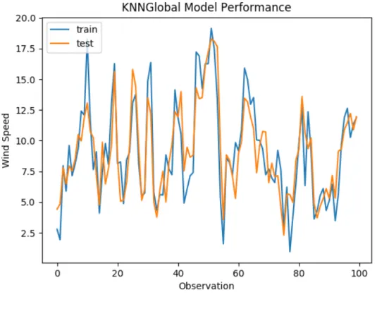
4.4.1.1 K Nearest Neighbors Model . . . 54

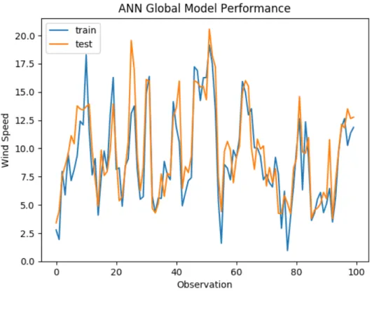
4.4.1.2 Artificial Neural Network Model . . . 56

4.4.2 Combined Models . . . 58

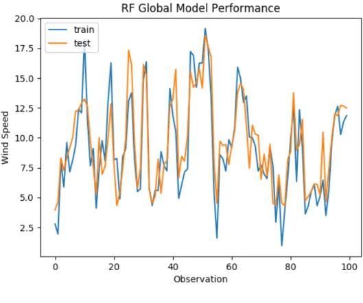
4.4.2.1 Random Forest Model. . . 58

4.4.2.2 Ensemble Model . . . 60

4.5 Local Models. . . 61

4.5.1 Clusters . . . 62

4.5.2 KNN Local models . . . 65

4.5.3 ANN Local models . . . 65

4.5.4 Random Forest Local models . . . 66

4.5.5 Ensemble Local models . . . 66

5 Discussion 69 5.1 Comparison of Single vs Combined Models . . . 69

5.1.1 kNN . . . 69

5.1.2 ANN . . . 69

5.1.3 Random Forest . . . 70

5.1.4 Ensemble . . . 70

5.1.5 Global comparison . . . 71

5.2 Comparison of Global vs Local Models . . . 71

5.2.1 k Nearest Neighbors . . . 71

5.2.2 ANN . . . 72

5.2.3 Random Forest . . . 73

(9)

5.3 Comparison among all Models . . . 74

5.4 Benchmark comparison . . . 76

6 Conclusions and Future Work 77 6.1 Conclusions . . . 77

6.2 Future work . . . 77

A Complementary Experiment results 79 A.1 Wind Speed Prediction using all 48F+M+H . . . 79

A.1.1 RandomForest Results . . . 79

A.1.2 kNN Results. . . 79

A.1.3 ANN Results . . . 79

A.2 Wind Speed Prediction with feature selection . . . 79

A.2.1 RandomForest Results . . . 80

A.2.2 kNN Results. . . 80

A.2.3 ANN Results . . . 81

(10)

(11)

List of Figures

2.1 Relationship between wind speed and wind power . . . 6

2.2 Physical Approach . . . 8

2.3 Statistical Approach. . . 10

2.4 Artificial Neural Network Approach . . . 11

2.5 Weighting-based combined approach . . . 14

2.6 Preprocessing combined approach . . . 15

2.7 Optimization combined approach . . . 16

2.8 Error processing combined approach . . . 16

2.9 UEB-1 algorithm . . . 22 2.10 UEB-2 algorithm . . . 23 2.11 RandomForest model . . . 29 2.12 Bagging algorithm . . . 30 2.13 Boosting algorithm . . . 31 2.14 Stacking algorithm . . . 31 2.15 Gesconda interface . . . 33

3.1 Data Science methodology . . . 38

3.2 Data preparation . . . 39

3.3 Methodology proposed. . . 40

3.4 Global modeling methodology proposed . . . 41

3.5 Single models . . . 41

3.6 Combined models. . . 42

3.7 Ensemble methodology proposed. . . 43

3.8 Methodology intuition . . . 44

3.9 Local modeling methodology proposed . . . 45

4.1 Wind farm location . . . 47

4.2 Atmospheric Pressure levels . . . 49

4.3 Wind Components . . . 50

4.4 Data Missing values . . . 51

4.5 Training process flowchart . . . 53

4.6 Testing process flowchart . . . 54

4.7 Global training process . . . 54

4.8 KNN Test Prediction . . . 56

4.9 ANN Test Prediction . . . 58

4.10 RandomForest Test Prediction . . . 60

4.11 Ensemble Test Prediction . . . 61

4.12 Local training process . . . 62

4.13 Train set clusters. . . 63

4.14 Test set clusters . . . 64

4.15 Sample of Cluster-1 data . . . 65

4.16 Sample of Cluster-2 data . . . 65

(12)

(13)

List of Tables

2.1 Comparison of the main methods. . . 13

2.2 Comparison of the combined approaches . . . 18

4.1 Variables . . . 48

4.2 Predictive Variables weights . . . 52

4.3 RandomForest feature selection results. . . 52

4.4 KNeighbors selection results. . . 52

4.5 KNeighbors CV training results under different k . . . 55

4.6 kNN test results for 20% unseen data. . . 56

4.7 ANN CV training results under different units . . . 57

4.8 ANN test results for 20% unseen data . . . 58

4.9 RandomForest CV training results under different decision trees. . . . 59

4.10 RandomForest test results for 20% unseen data . . . 60

4.11 Ensemble test results for 20% unseen data . . . 61

4.12 Clusters partition . . . 64

4.13 Local KNN model test results for 20% unseen data . . . 66

4.14 Local ANN model test results for 20% unseen data . . . 66

4.15 Local RF model test results for each cluster of 20% unseen data . . . . 66

4.16 Local Ensemble model test results for each cluster of 20% unseen data 67 5.1 Global KNN model test results for 20% unseen data . . . 69

5.2 Global ANN model test results for 20% unseen data . . . 70

5.3 Global RF model test results for 20% unseen data. . . 70

5.5 Single vs Combined Models . . . 71

5.6 Global KMM model test results for each cluster . . . 72

5.7 Local KNN model test results for 20% unseen data . . . 72

5.8 Global ANN model test results for each cluster . . . 72

5.9 Local ANN model test results for 20% unseen data . . . 73

5.10 Global RF model test results for each cluster. . . 73

5.11 Local RF model test results for each cluster of 20% unseen data . . . . 74

5.13 Local Ensemble model test results for each cluster of 20% unseen data 74 5.14 Comparison Among all Models . . . 75

5.15 Comparative best results of the wind power estimation by the ELM and GPR . . . 76

A.1 RandomForest results using all 48F+M+H . . . 79

A.2 kNN results using all 48F+M+H . . . 80

A.3 ANN results using all 48F+M+H . . . 80

A.4 Predictive Variables weights . . . 81

A.5 RandomForest results with feature selection. . . 81

(14)

(15)

List of Abbreviations

RF RandomForest

kNN K NearestNeighbors

(16)

(17)

(18)

(19)

Chapter 1

Introduction

This chapter explains the main motivation of our work, as well as the main goal proposed for the work.

1.1

Motivation

Development of alternative energy sources has become a necessity as fossil energy resources are declining. At the same time, energy demand is rapidly increasing, putting the world on the verge of a global energy crisis. Moreover, the extensive use of conventional energy sources is polluting the environment and causing global warming. On the other hand, wind and other renewable energy sources are viable and clean alternatives to fossil fuels. Low operating cost and extensive availability make wind one of the most advantageous and effective renewable energy sources [1].

Wind energy is of vital importance among the low-carbon energy technologies, which has the potential to achieve sustainable energy supply and constitutes a key-stone component for micro-grids in a way towards the smart grid infrastructure. However, stochastic and intermittent wind power generation poses a number of challenges to the large scale penetration of wind power. These wind-related uncer-tainties can put the system reliability and power quality at risk with the increasing penetration of wind power and thus, the main grid integration issues such as bal-anced management and reserve capacities can come into question [2,3,4]. Reducing the need for balancing energy and making the power generation scheduling and dispatch decisions can be realized with the help of wind speed and power gener-ation forecasts [5]. Furthermore, the forecasts can play a vital role in keeping the costs competitive by reducing the need for wind curtailments and thereby, increas-ing revenue in electricity market operations [6]. However, the random and unstable characteristics of the wind make it considerably difficult to forecast the wind speed and power accurately. Hence, extensive efforts have been devoted for the devel-opments and improvements of wind speed and power forecasting approaches by numerous energy and environment related research centers and universities [7].

In the literature, many forecasting approaches have been studied and proposed, each utilizing a different technique and performing well with a different prediction horizon. Recent studies in the area of wind prediction are predominantly focused on the short-term wind predictions ranging from minutes to a few days due to the importance of these data on power systems [7]. Especially day-ahead predictions are of significant interest for system operations such as scheduling, unit commit-ment and load following [8,9]. However,it is generally difficult to accomplish such a long-term prediction and moreover, the approaches designed for long prediction horizons maybe deficient for shorter terms in terms of prediction performance. Fol-lowing many studies in the wind forecasting field, it can be indicated that, to date,

(20)

the targeted performance levels have not been attained with the individual models due to the fact that these models can not give satisfactory results for all situations. For instance, the physical models produce coarse predictions for short-term hori-zons while mostly outperform the other models in medium and long-term horihori-zons. Also, Artificial Intelligence (AI) based models that rely on a large number of his-torical data for constructing an input/output mapping function can be less effective than some basic conventional statistical methods for certain application areas in the case of inadequate available information. Therefore, the approaches that incorpo-rate the individually superior features of various forecasting models have emerged, called as hybrid models and combined models, in order to obtain an advanced fore-casting method for higher accuracy levels and wider forecast horizons [7].

After evaluating the findings of the studies on the hybrid models, which will be detailed in next chapter, it can be concluded that these models do not generally con-tribute to the forecasting performance of the individual models considerably and they can even lead to poor performances under some circumstances [10]. On the other hand, combined forecasting methodologies, which follow a different approach and produce the final forecast generally from the weighting of the single approaches, can be a more viable solution for improving the accuracy of the individual mod-els. To that end, the search effort has been recently oriented towards designing new combined algorithms as well as combination methods, which exploit different sin-gle prediction models and enhance the prediction performance while providing a reasonable computation time. A study on the classifying and summarizing of the combined methods, which might give an insight about the performance, superior-ity and application area of various algorithms, was presented in [7] which we will review in order to base this work.

1.2

Goal

With the continuous increase of wind power penetration in power systems, the prob-lems caused by the volatile nature of wind speed and its occurrence in the system operations such as scheduling and dispatching have drawn attention of system op-erators, utilities and researchers towards the state-of-the-art wind speed and power forecasting methods. These methods have the required capability of reducing the influence of the intermittent wind power on system operations as well as of harvest-ing the wind energy effectively. In this context, combinharvest-ing different methodologies in order to circumvent the challenging model selection and take advantage of the unique strength of plausible models have recently emerged as a promising research area [7].

In this work, we present a comprehensive exploration about machine learning models including global and local, as well as combined models and how these mod-els are constructed and affect the forecasting performance and final Wind Speed Pre-diction.

The goal is to explore which are the best models among all ones trying to get the estimation of the Wind Speed Prediction. Furthermore, we want to draw some conclusions from the study.

(21)

Chapter 2

State of Art

In this chapter the state of the art related to the work done is presented. First, the domain were the machine learning models has been applied i.e. the Wind Speed prediction problem is presented. Afterwards the different methodologies applied in the Wind Speed prediction problem are explained. Finally, main machine learning techniques are detailed.

2.1

Wind Prediction Problem

2.1.1 Wind Farms

A wind farm is the site where a group of wind turbines are installed for bulk elec-tricity generation. Nameplate capacity of modern wind parks has increased by up to thousands of MWs. Wind farms can be categorized asonshoreandoffshorebased on the location where wind turbines are installed.

Any wind power system typically comprises of wind turbines, generators, power transformers, and a connection to the power grid [11]. There are usually three kinds of wind systems: the constant speed wind turbine system with a standard squir-rel cage induction generator (SCIG), the variable speed wind turbine system with a double-fed induction generator (DFIG), and the variable speed wind turbine with a full rated power electronics conversion system and a synchronous generator [1]. 2.1.2 Wind Prediction

A wind power forecast corresponds to an estimate of the expected production of one or more wind turbines referred to as a wind farm. By production is often meant available power for wind farm considered (with units kW or MW depending on the wind farm nominal capacity). Forecasts can also be expressed in terms of energy, by integrating power production over each time interval [12].

2.1.2.1 Time scales of forecasts

The basic role of wind speed and power forecasting is to provide information about the wind speed and power that can be expected in the next few minutes, hours, or days. Based on power system operation requirements, the forecast can be divided into four different horizons: very short-term (few seconds to 30 min), short-term (30 min to 6 h), medium-term (6–24 h), and long-term (1–7 days). [13, 14] Very short-term forecasts are used for turbine control and load tracking. Short-short-term forecasts are utilized for preload sharing. Medium-term forecasts are used for power sys-tem management and energy trading. Long-term forecast are used for maintenance scheduling of the wind turbines.

(22)

For the last two possibilities, the temporal resolution of wind power predictions ranges between 10 minutes and a few hours (depending on the forecast length). Im-provements of wind power forecasting has focused on using more data as input to the models involved, and on providing uncertainty estimates along with the tradi-tionally provided predictions [12].

2.1.3 Reason for wind forecasts

As detailed in [12], in the electricity grid at any moment balance must be maintained between electricity consumption and generation - otherwise disturbances in power quality or supply may occur. Wind generation is a direct function of wind speed and, in contrast to conventional generation systems, is not easily dispatchable. Fluc-tuations of wind generation thus receive a great amount of attention. Variability of wind generation can be regarded at various time scales. First, wind power produc-tion is subject to seasonal variaproduc-tions, i.e. it may be higher in winter in Northern Europe due to low-pressure meteorological systems or it may be higher in summer in the Mediterranean regions owing to strong summer breezes. There are also daily cycles which may be substantial, mainly due to daily temperature changes. Finally, fluctuations are observed at the very short-term scale (at the minute or intra-minute scale). The variations are not of the same order for these three different timescales. Managing the variability of wind generation is the key aspect associated to the opti-mal integration of that renewable energy into electricity grids.

The challenges to face when wind generation is injected in a power system de-pend on the share of that renewable energy. It is a basic concept, the wind penetra-tion which allows one to describe the share of wind generapenetra-tion in the electricity mix of a given power system. For Denmark, which is a country with one of the high-est shares of wind power in the electricity mix, the average wind power penetration over the year is of 16-20% (meaning that 16-20% of the electricity consumption is met wind energy), while the instantaneous penetration (that is, the instantaneous wind power production compared to the consumption to be met at a given time) may be above 100%.

The transmission system operator (TSO) is responsible for managing the electric-ity balance on the grid: at any time, electricelectric-ity production has to match consump-tion. Therefore, the use of production means is scheduled in advance in order to respond to load profiles. The load corresponds to the total electricity consumption over the area of interest. Load profiles are usually given by load forecasts which are of high accuracy. For making up the daily schedule, TSOs may consider their own power production means, if they have any, and/or they can purchase power gener-ation from Independent Power Producers (IPPs) and utilities, via bilateral contracts or electricity pools. In the context of deregulation, more and more players appear on the market, thus breaking the traditional situation of vertically-integrated utilities with quasi local monopolies. Two main mechanisms compose electricity markets. The first one is the spot market where participants propose quantities of energy for the following day at a given production cost. An auction system permits to settle the electricity spot price for the various periods depending on the different bids. The second mechanism is the balancing of power generation, which is coordinated by the TSO. Depending on the energy lacks and surplus (e.g. due to power plant failures or to intermittence in the case of wind power installations), the TSO deter-mines the penalties that will be paid by IPPs who missed in their obligations. In some cases, an intra-day market is also present, in order to take corrective actions.

(23)

In order to illustrate this electricity market mechanism, let us consider the Dutch electricity market. Market participants, referred to as Program Responsible Parties (PRPs), submit their price-quantity bids before 11 am for the delivery period cover-ing the followcover-ing day from midnight to midnight. The Program Time Unit (PTU) on the balancing market is of 15 minutes. Balancing of the 15-minute averaged power is required from all electrical producers and consumers connected to the grid, who for this purpose may be organized in subsets. Since these subsets are referred to as Programmes, balancing on the 15-minute scale is referred to as Programme Balance. Programme Balance now is maintained by using the production schedules issued the day before delivery and measurement reports (distributed the day after deliv-ery). When the measured power is not equal to the scheduled power, the Programme Imbalance is the difference between the realised sum of production and consump-tion and the forecast sum of producconsump-tion and consumpconsump-tion. If only producconsump-tion from wind energy is taken into account, Programme Imbalance reduces to release wind production minus forecast wind production. The programme imbalance is the wind production forecast error.

Programme Imbalance is settled by the System Operator, with different tariffs for negative Programme Imbalance and positive Programme Imbalance. A positive Pro-gramme Imbalance indicates more energy actually produced than forecast. by wind energy the realised wind production is bigger than the forecast wind production. And vice versa, in the case of a negative Programme Imbalance by wind energy.

Note that the costs for positive and negative imbalances may be asymmetric, depending on the balancing market mechanism. In general, wind power producers are penalized by such market system since a great part of their production may be subject to penalties.

In parallel to be used for market participation, wind power forecasts may be used for the optimal combined operation of wind and conventional generation, wind and hydro-power generation, or wind in combination with some energy storage devices. They also serve as a basis for quantifying the reserve needs for compensating the eventual lacks of wind production.

2.1.4 Relationship between wind speed and wind power

Wind power is directly related to the wind speed through a so-called power curve

2.1. This is a simplified way of expressing the wind power in terms of atmospheric variables. Other atmospheric fields, such as wind shear, turbulence and air density have also impact on the actual power production for a given wind speed. However, for wind power verification wind speed is the most important parameter, because the bulk of the prediction error is caused by the wind speed prediction errors [15].

(24)

FIGURE2.1: Relationship between wind speed and wind power (Ex-tracted from [15]).

Given this relationship between wind speed and wind power generation, the efforts in our work will be focused on the prediction of the wind speed variable, because is the fundamental feature for the wind power generation.

2.2

Wind Prediction Methodology

As detailed in [12], several methods are used for short-term prediction of wind gen-eration. The simplest ones are based on climatology or averages of past production values. They may be considered as reference forecasting methods since they are easy to implement, as well as benchmark when evaluating more advanced approaches. The most popular of these reference methods is certainly persistence. This naive predictor — commonly referred to as "what you see is what you get" — states that the future wind generation will be the same as the last measured value. Despite its apparent simplicity, this naive method might be hard to beat for look-ahead times up to 4–6 hours ahead.

Advanced approaches for short-term wind power forecasting necessitate predic-tions of meteorological variables as input. Then, they differ in the way predicpredic-tions of meteorological variables are converted to predictions of wind power production, through the so-called power curve. Such advanced methods are traditionally di-vided into two groups:

• The first group, referred to as physical approach, focuses on the description of the wind flow around and inside the wind farm, and use the manufacturer’s power curve, for proposing an estimation of the wind power output.

• The second group, referred to as statistical approach1, concentrates on captur-ing the relation between meteorological predictions (and possibly historical measurements) and power output through statistical models whose parame-ters have to be estimated from data, without making any assumption on the physical phenomena.

2.2.1 Prediction of meteorological variables

As details in [12] Wind power generation is directly linked to weather conditions and thus the first aspect of wind power forecasting is the prediction of future values of 1_{Although in the literature they are named as statistical forecasting methods they include also}

ma-chine learning techniques. Therefore, it would be better to name them as data-driven forecasting meth-ods

(25)

the necessary weather variables at the level of the wind farm. This is done by using numerical weather prediction (NWP) models. Such models are based on equations governing the motions and forces affecting motion of fluids. From the knowledge of the actual state of the atmosphere, the system of equations allows to estimate what the evolution of state variables, e.g. temperature, velocity, humidity and pressure, will be at a series of grid points. The meteorological variables that are needed as input for wind power prediction obviously include wind speed and direction, but also possibly temperature, pressure and humidity. The distance between grid points is called the spatial resolution of the NWPs. The mesh typically has spacing that varies between few kilometers and up to 50 kilometers for mesoscale models. Re-garding the time axis, the forecast length of most of the operational models today is between 48 and 172 hours ahead, which is in adequacy with the requirements for the wind power application. The temporal resolution is usually between 1 and 3 hours. NWP models impose their temporal resolution to short-term wind power forecasting methods since they are used as a direct input.

Predictions of meteorological variables are provided by meteorological institutes. Meteorologists employ atmospheric models for weather forecasts on short and medium term periods. An atmospheric model is a numerical approximation of the physical description of the state of the atmosphere in the near future, and usually is run on a supercomputer. Each computation starts with initial conditions originating from recent measurements. The output consists of the expected instantaneous value of physical quantities at various vertical levels in a horizontal grid and stepping in time up to several hours after initiation. There are several reasons why atmospheric models only approximate reality. First of all, not all relevant atmospheric processes are included in the model. Also, the initial conditions may contain errors (which in a worse case propagate), and the output is only available for discrete points in space (horizontal as well as vertical) and time. Finally, the initial conditions age with time - they are already old when the computation starts let alone when the output is published. Predictions of meteorological variables are issued several times per day (commonly between 2 and 4 times per day), and are available few hours after the be-ginning of the forecast period. This is because some time is needed for acquiring and analyzing the wealth of measurements used as input to NWP models, then run the model and check and distribute the output forecast series. This gap is a blind spot in the forecasts from an atmospheric model. As an example in the Netherlands, KNMI publishes 4 times per day expected values of wind speed, wind direction, tempera-ture and pressure for the period the between 0 and 48 hours after initialization of the atmospheric model Hirlam with measured data, and then the period before forecast delivery is of 4 hours.

Many different atmospheric models are available, ranging from academic re-search tools to fully operational instruments. Besides for the very nature of the model (physical processes or numerical schemes) there are some clear distinctive differences between them: time domain (from several hours to 6 days ahead), area (several 10.000 km2 to an area covering half the planet), horizontal resolution (1 km to 100 km) and temporal resolution (1 hour to several hours).

One of the atmospheric models is the High Resolution Limited Area Model, ab-breviated HiRLAM, which is frequently used in Europe. HiRLAM comes in many versions, that’s why it is better to speak about "a" HiRLAM rather than "the" HiRLAM. Each version is maintained by a national institute such as the Dutch KNMI, the Dan-ish DMI or FinnDan-ish FMI. And each institute has several versions under her wing, divided into categories such as: operational, preoperational, semi operational and for research purposes.

(26)

Other atmospheric models are UKMO in the UK, Lokalmodell in Germany, Al-ladin in France (AlAl-ladin and Lokalmodell are also used by some other country’s within Europe), and MM5 in the USA.

2.2.2 Main Approaches

Research in the area of forecasting wind speed produced by wind farms has been devoted to the development of effective and reliable tools and many different ap-proaches have been proposed. These tools can be classified whether the terrain in-formation at the location is used as an input or not. Two mainstream approaches are thephysical and the statistical approach. In some models acombination approachis used in an attempt to integrate the advantages of both approaches. In this section an overview of existing wind speed forecast approaches is presented [16].

2.2.2.1 Physical forecasting approach or Mechanistic model-driven

The physical approach to forecasting, in contrast to statistical approach, uses the detailed physical description to model the on-site conditions at the location of the wind farm [17,18]. The basic operation of a physical approach is illustrated in Fig.

2.2.

FIGURE 2.2: The physical approach to forecasting wind speed and power (Extracted from [16]).

It carries out the refinement of the Numerical Weather Prediction (NWP) data to take into account the on-site conditions by the downscaling method, which are based on the physics of the lower atmospheric boundary layer. The downscaling method

(27)

requires the detailed physical descriptions of the wind farms and their surroundings, including: description of the wind farm (wind farm layout and wind turbine power curve, etc.) and description of the terrain (orography, roughness, obstacles, etc.). Then, the refined wind speed data at the hub height of the wind turbines is plugged into the corresponding wind power curve to calculate the wind power production. If the on-line data is available, model output statistics are performed to reduce the error of the forecast. Contrary to the statistical approach, the physical approach does not require training input from historical data. However, acquiring the physical data is one of the main drawbacks of the approach [16].

A number of physical approaches have been introduced in [16]. The Predik-tor is developed by the Risoe National LaboraPredik-tory in Denmark. It uses Wind At-las Analysis and Application Program (WAsP) and PARK program to take the local conditions into account by using the NWP forecast from High Resolution Limited Area Model (HIRLAM) [19]. The Previento, developed by the University of Olden-burg in Germany has a similar physical approach but uses a different NWP forecast from Lakelmodell of the German Weather Service [20]. The LocalPred is developed by CENER – National Renewable Energy Centre in Spain. It involves adaptive op-timization of the NWP forecast, time series modeling, meso-scale modeling with MM5, and power curve modeling [21]. The eWind, developed by AWS TrueWind Inc. in the USA, has a similar physical approach with Prediktor but uses a high-resolution boundary layer model (ForeWind) as a numerical weather model to take the local conditions into account [22].

The physical approaches are based on the models using the fundamental physi-cal principles for conservation of mass, momentum, and energy in air flows. These models address computational fluid dynamics (CFD) for simulating the atmosphere. Although there are many CFD models available, they are all based on the same basic physical principles. They differ in how the grids are structured and scaled, and how the numerical computations are performed [16].

In the majority of cases the statistical approaches provide good results in short-term, medium-short-term, and long-term forecasting. However, in the very short-term and short-term horizon, the influence of atmospheric dynamics becomes more im-portant, and in these cases the use of physical approaches becomes essential.

2.2.2.2 Statistical forecasting approach or Data-driven

The alternative main approach for wind speed and power forecasting is based on statistical modeling. The statistical approach represents the relation between wind power or speed forecasting and explanatory variables including NWPs and on-line measured data [17]. The general form of the model is illustrated in Fig.2.3.

(28)

FIGURE2.3: The statistical approach to forecasting wind speed and power (Extracted from [16]).

The statistical approach generally uses previous history data to build the statis-tical model. This model uses NWP forecast for time t+k and on-line measurement at time t to forecast the present over the next few hours. It is easy to model and inexpensive. However, contrary to the physical approach, the statistical approach requires historical data to train the statistical model. Many different approaches are employed [16]. Some of the most representative statistical approaches are reviewed in this section.

2.2.2.2.1 Conventional statistical approach

In the conventional statistical approach a time series model is applied to forecast future wind power or speed. According to the forecasting process, which was pro-posed by Box–Jenkins, this model is divided into four main steps to make a math-ematical model of the problem including model identification, model estimation, model diagnostics checking, and forecasting. Several types of time series models may be considered, including autoregressive model (AR), moving average model (MA), autoregressive moving average model (ARMA), and autoregressive integrated moving average model (ARIMA). The general form of the model is:

Xt =c+εt+ p

∑

i=1 ϕXt−i+ q

∑

i=1 θiεt−i (2.1)

whereXtrepresents the forecasting parameter at timet, ϕ_i is the autoregressive

parameter,θi is the moving average parameter,cis the constant, and random

vari-ableεtis the white noise. This model represents the ARMA model having the

autore-gressive model of orderp and the moving average model of orderq(ARMA(p,q)). If the order of the moving average model (q) is zero, it represents the autoregres-sive model of orderp (AR(p)). If the order of the autoregressive model (p) is zero,

(29)

it represents the moving average model of order q (MA(q)). The ARIMA model is a generalization of an ARMA model [16].

2.2.2.2.2 Artificial Neural Network approach

Another common approach is based on the use of Artificial Neural Networks (ANN). The NWP forecasts and further meteorological variables are transformed into the wind power or speed forecast by ANN which has been trained by the large sets of historical data in order to learn the dependence of the output on input variables. The general ANN approach for wind speed and power forecast is shown in Fig.2.4.

FIGURE2.4: ANN approach for wind speed and power forecast (Ex-tracted from [16]).

ANN is one of the widely used statistical approaches for wind speed and power forecasts. It consists of an input layer, one or more hidden layers, and an output layer. Each layer has a number of artificial neurons, and it uses a connectionist ap-proach to connect the neurons to the neurons of the previous layer. This apap-proach is able to model the complex non-linear relationship between the input and output layers through a training and learning process. This approach does not require ex-plicit mathematical expressions as used in the physical and statistical approaches reviewed previously. Furthermore, it has the ability of self-learning, self-organizing and self-adaption [16].

2.2.2.3 Comparison

As indicated above, the underlying idea behind combining models can be described as the utilization of the features of different forecasting methods. In this context, it is reasonable to first briefly mention the most widely used forecasting methods in the literature and their characteristics. To this end, the forecasting methods are classified according to the common terminology criteria for wind forecasting methods and inspected by several studies from the literature [7].

The majority of the wind forecasting techniques can be clustered into two main groups, namelyphysical methodsandstatistical methods. In short, the first group takes into account the physical considerations such as local terrain, wind farm layout and temperature to reach the estimate and utilizes the output from Numerical Weather

(30)

Prediction (NWP) models which provide weather forecasts by using the mathemat-ical model of the atmosphere. The concept of utilizing the NWP models as an input was taken into account by Landberg and then corrections on the wind speed predic-tions were applied by making use of various programs such as Wind Atlas Analysis and Application Program (WAsP) and PARK [23]. Furthermore, the NWP model output can be used directly for wind speed predictions, as demonstrated in [24]. Likewise, another NWP model, called as Eta Model, was utilized for wind predic-tion up to 36 h in [15] and it was shown that Eta model is quite effective in predicting wind energy.

The latter aims at describing the relation between historical time series of wind speed (or power) at the location of interest by generally recursive techniques and it can be stated that short term forecasting models are generally based on statistical approaches due to the fact that NWP models require long operation time and large amount of computational resources.

As can be seen from the mentioned research and review studies, each forecasting model has its own strengths and weaknesses over the other models. In order to gather the present knowledge on the widely used wind forecasting models in the literature, a concise comparison of these basic approaches is shown in Table2.1. 2.2.3 Combination Approaches

The basic idea of thecombination modelis to combine different strategies or models, retaining advantages of each approach. The desire is to improve the forecast accu-racy, but combining forecasts does not always perform better than the best individ-ual forecasts. However, in some cases it is viewed as less risky to combine forecasts than to select just an individual forecast [25].

Several approaches have been developed based on the combination of various models [16]. As stated earlier, combined forecasting methodologies can improve the final forecasting performance taking advantages of individual forecasting methods which have different performances depending on the data sets, forecast horizons as well as their capability of capturing nonlinearity, and provide some advantages com-pared to the individual methods. Among the advantages, the potential of utilizing the combined methods in a wider range of application area has a special importance due to the fact that individual models perform well only in a certain situation and therefore different models have to be tested for deciding the most suitable one. The mentioned time consuming drawback of individual methods can be overcome while using combined models, particularly in the case that the determination of the best performing model is complicated.

There is controversy and confusion in the literature about the definition and structure of the combined models. Notwithstanding, it can be indicated that the most widely accepted procedure for combination of models taking place in the lit-erature is to assign a weighting coefficient to each method proportional to their past forecasting performance. Besides, some other approaches are presented as combined models in the literature of wind forecasting by utilizing different methodologies. The mentioned weighting and other combination methods are elucidated and exem-plified in detail according to a chronological sequence and by grouping the similar studies, correspondingly in the following sections [7].

(31)

TABLE2.1: Brief comparison of the main methods used for forecast-ing of wind speed in the literature (Extracted from [7].)

Wind speed forecast-ing approach

Advantages Disadvantages

NWP models Applicable for longer predic-tion horizons

Weakness in handling smaller scale phenomena, not suitable for short fore-cast times, requires large computational resource and time

Time series models (AR, ARMA, ARIMA, f-ARIMA, etc.)

Easy to find tools, compar-atively basic structure, ca-pability of correcting local trends in data, provides con-fidence intervals for predic-tions

Requires a great deal of historic records, difficult to model nonlinear problems and decide the best structure

ANN-based models Gains knowledge from train-ing data, no need to spec-ify any mathematical model a priori, high data error tol-erance, higher adaptability to online measurements

Requires a training procedure and a large number of train-ing data

SVM-based models High generalization perfor-mance

Depends on the tuning of parameters appropriately, complex optimization pro-cess and longer training time

Fuzzy logic models Suitable for systems which are difficult to model exactly, relatively less complex

High complexity and a long process time in the case of many rules

Bayesian networks Ability to handle missing ob-servations and to avoid the overfitting of data, suitable for small training data sets, suitable for various input data

Requires relatively more ef-fort, depends on the user’s expertise level

Kalman filter models Does not require to store all historic data because of its re-cursive form

Requires previous knowl-edge about the system

(32)

2.2.3.1 Weighting-based combined approaches

From a conceptual point of view, the process of weighting used for the combina-tion of the wind forecasting models can be defined as determining the relative effec-tiveness of each model and providing them an appropriate value that reflects their special importance in the combined model. The general prediction process of these combined models is depicted in Fig.2.5.

FIGURE2.5: Flowchart of the weighting-based combined approaches. (Extracted from [7])

2.2.3.2 Other combined approaches

In the literature, these approaches generally consist of two different models, one for main forecasting task and the other for the auxiliary processes such as data filtering, data decomposition, selection of the best parameter and residual error evaluation. Depending on the function of the models used for the auxiliary processes in the final model, “the other combined approaches” can be gathered into three groups:

• combined approaches including data preprocessing techniques,

• combined approaches including parameter selection and optimization tech-niques, and

• combined approaches including data post-processing techniques [7].

2.2.3.2.1 Combined approaches including data preprocessing techniques

In the first group, the main objective of the data pre-processing models is, as the name implies, to realize a preliminary process on data sets by decomposing the non-linear wind speed time series into more stationary and regular subseries which are generally easier to analyze and/or by filtering out the irrelevant and redundant fea-tures of the data set. Thus, more stable subseries are obtained as well as the most

(33)

informative training data is determined enabling to improve the quality of the data and avoiding the unnecessary computation burden. The basic flowchart followed in a large part of the mentioned approaches is illustrated in Fig.2.6.

FIGURE2.6: Flowchart of combined approaches including data pre-processing techniques (Extracted from [7]).

2.2.3.2.2 Combined approaches including parameter selection and optimization techniques

In a large numbers of papers on wind forecasting, it has been reported that cer-tain parameter selection and optimization approaches also can make a considerable contribution to the prediction performance during the training process. The selec-tion of explanatory variables and determinaselec-tion of model parameters while using the mentioned approaches can allow avoiding the time consuming process of the optimization of the prediction method, which is usually carried out by testing the method over a large number of candidate parameters and deriving the structure of the model heuristically. The approaches in question perform the predictions after a parameter evaluation process with a suitable method, as shown in Fig.2.7.

(34)

FIGURE2.7: Flowchart of combined approaches including parameter selection and optimization techniques. (Extracted from [7])

2.2.3.2.3 Combined approaches including error processing techniques

Apart from the approaches mentioned before, there exists a few combined approaches in the literature that have a structure that takes into account the residual error values obtained from a forecasting model, as denoted in Fig.2.8.

FIGURE2.8: Flowchart of combined approaches including error pro-cessing techniques (Extracted from [7]).

2.2.3.3 Comparison

In the literature, there exist a lot of studies on the predictions of wind speed and power with various methods, which mostly generate reasonable values and each method has its own advantages and disadvantages. However, due to the fact that the prediction models developed are generally site-specific and considerably influenced by the changing of required prediction times, the suitable model is selected regard-ing the specific data characteristic of the site and the application area of the method with a time-consuming and specialist process. In order to address this problem by avoiding the ambiguity of model selection and to further improve the prediction performance, combining several methods have been proposed, especially at the last years and the results obtained have verified the effectiveness of these approaches. The subject of combined wind speed and power forecasting methods can be deemed

(35)

as a novel research area. Therefore, a consensus has not yet been reached concern-ing the fundamentals of the subject and the basic definitions about the related terms. For instance, it can be readily indicated that predictions errors are always propor-tional to the prediction time; however, it is not possible to say exactly which method is the most appropriate candidate for a certain prediction time. In this issue, only some suggestions and assumptions are available at this stage. Likewise, the clas-sification of the methods according to the prediction time is another subject that is suggested in various ways in the literature. For instance, the short term prediction is defined as the predictions up to six-hour-ahead in [26]; however, it corresponds to 24-h-ahead predictions in [27] and 72-h-ahead predictions in [9]. Besides, com-parison of the forecasting performance of the models is another troublesome topic evidently due to the fact that no single model provides the best predictions in terms of all performance metrics, meaning that a universal standard for a fair comparison of prediction performances is not yet present [7].

Similar to the above mentioned problems, it is important to highlight that there still exist discrepancies in the definitions and structures of the combined and hybrid forecasting approaches and this situation complicates the classification and compar-ison of the approaches. For this purpose, the approaches were divided into several main and sub-categories and the effects of different models on the forecasting per-formance are briefly described and discussed by pursuing an extensive body of the literature in this direction [7]. According to the mentioned studies, firstly there is no doubt that combination of proper prediction techniques is of significant importance in terms of improving the accuracy. Then, the preliminary processing of the input data, particularly with decomposing and filtering methods such as a Wavelet Trans-form (WT) and EMD (Empirical Mode Decomposition) methods, has been found valuable for facilitating the forecasting process and thereby, improving the predic-tion quality with the cost of spending more time on final model building. Likewise, it was observed that evolutionary algorithms such as GA (Genetic Algorithms), EP (Evolutionary Programming) and DE (Differential Evolution) methods and Kalman filtering method tend to perform well for the selection and optimization of the pre-diction system parameters. Moreover, it was realized that the total performance of the prediction methods can be augmented by also predicting and then including the residual error values with a variety of models. A brief evaluation about each class of the combined approaches which is determined according to the above mentioned criterion is shown in Table2.2[7].

By examining the characteristics of the combined approaches summarized in Ta-ble 2, it can be concluded that the approaches with a weighting model and with a data preprocessing model are very suitable for longer and harder prediction tasks, which are required for power system operations such as scheduling, unit commit-ment and load following. Weighting-based approaches consisting of an NWP model should also be utilized effectively for the much longer term objectives such as main-tenance of wind turbines or conventional power plants. Besides, the approaches including parameter selection and data optimization techniques may present high-accuracy predictions required mainly for energy trading and marketing. However, the approaches with an error processing method may only give reasonable results in the case of systematic errors and hence are not of a specific application area. Lastly, it is worth mentioning that the combined models are ineffective in very short term forecasts, ranging from milliseconds up to a few minutes and used for wind turbine active control, due to the fact that these approaches have generally computational time inefficiency compared to the individual methods [7].

(36)

TABLE2.2: Brief evaluation of combined approaches applied for fore-casting of wind speed in the literature (Extracted from [7]).

Combined wind speed forecast-ing approach

Strategy Advantages Disadvantages

Weighting-based combined ap-proaches Assigning weight factors to models according to their performance Easy to imple-ment and code, suitable for a wide range of prediction time, adaptive to new data

Does not guar-antee the best predictions along the prediction horizon, requires an extra model for determining the weights Combined ap-proaches in-cluding data preprocessing techniques Forecasting of the subseries obtained by decomposition models Higher perfor-mance compared to other ap-proaches, easy to find literature examples, ro-bustness to rapid changes in wind speed Requires a de-tailed mathemat-ical knowledge on decompo-sition models, provides slow response to new data Combined ap-proaches includ-ing parameter selection and optimization techniques Optimization of the parameters of forecasting model

Easy to find lit-erature examples, a relatively basic structure Harder to code, dependent on de-signer’s knowl-edge about the optimization problems, com-putationally intensive Combined ap-proaches in-cluding error processing tech-niques Forecasting of residual error caused by fore-casting model High accuracy, effective in reducing system-atic error Computational time inefficiency

(37)

2.3

Atmospheric Reanalysis Data

Reanalysis is a systematic approach to produce data sets for climate monitoring and research. Reanalyses are created via an unchanging ("frozen") data assimila-tion scheme and model(s) which ingest all available observaassimila-tions every 6-12 hours over the period being analyzed. This unchanging framework provides a dynami-cally consistent estimate of the climate state at each time step. The one component of this framework which does vary are the sources of the raw input data. This is un-avoidable due to the ever changing observational network which includes, but is not limited to, radiosonde, satellite, buoy, aircraft and ship reports. Currently, approx-imately 7-9 million observations are ingested at each time step. Over the duration of each reanalysis product, the changing observation mix can produce artificial vari-ability and spurious trends. Still, the various reanalysis products have proven to be quite useful when used with appropriate care [28].

Key Strengths

• Global data sets, consistent spatial and temporal resolution over 3 or more decades, hundreds of variables available; model resolution and biases have steadily improved

• Reanalyses incorporate millions of observations into a stable data assimilation system that would be nearly impossible for an individual to collect and analyze separately, enabling a number of climate processes to be studied

• Reanalysis data sets are relatively straightforward to handle from a processing standpoint (although file sizes can be very large)

Key Limitations

• Observational constraints, and therefore reanalysis reliability, can considerably vary depending on the location, time period, and variable considered

• The changing mix of observations, and biases in observations and models, can introduce spurious variability and trends into reanalysis output

• Diagnostic variables relating to the hydrological cycle, such as precipitation and evaporation, should be used with extreme caution

2.3.1 European Centre for Medium-Range Weather Forecasts

The European Centre for Medium-Range Weather Forecasts (ECMWF) is an inde-pendent intergovernmental organisation supported by 34 states.

ECMWF is both a research institute and a 24/7 operational service, producing and disseminating numerical weather predictions to its Member States. This data is fully available to the national meteorological services in the Member States. The Centre also offers a catalogue of forecast data that can be purchased by businesses worldwide and other commercial customers. The supercomputer facility (and asso-ciated data archive) at ECMWF is one of the largest of its type in Europe and Member States can use 25% of its capacity for their own purposes.

The organisation was established in 1975 and now employs around 350 staff from more than 30 countries. ECMWF is one of the six members of the Co-ordinated Organisations, which also include the North Atlantic Treaty Organisation (NATO),

(38)

the Council of Europe (CoE), the European Space Agency (ESA), the Organisation for Economic Co-operation and Development (OECD), and the European Organisation for the Exploitation of Meteorological Satellites (EUMETSAT).

ECMWF is based in Reading, UK. What they produce:

• produce numerical weather forecasts and monitor the Earth-system;

• carry out scientific and technical research to improve forecast skill;

• maintain an archive of meteorological data. To do so the Centre provides:

• twice-daily global numerical weather forecasts;

• air quality analysis;

• atmospheric composition monitoring;

• climate monitoring;

• ocean circulation analysis;

• hydrological prediction.

2.3.1.1 ERA-Interim

ERA-Interim is a global atmospheric reanalysis data from 1979, continuously up-dated in real time.

The data assimilation system used to produce ERA-Interim is based on a 2006 release of the IFS (Cy31r2). The system includes a 4-dimensional variational analysis (4D-Var) with a 12-hour analysis window. The spatial resolution of the data set is approximately 80 km (T255 spectral) on 60 vertical levels from the surface up to 0.1 hPa.

ERA-Interim data can be downloaded from the ECMWF Public Datasets web interface or from MARS (class=ei, expver=1).

For a detailed documentation of the ERA-Interim Archive see [29] .

2.4

Machine Learning techniques used

In this section we proceed to explain the algorithms that are going to be used on our proposed methodology.

Firstly, we will detail the unsupervised techniques which are the ones used for feature weighting called Unsupervised Entropy-base method and also the one used to create the clusters which will be used to train and test our local models.

Later, we will detail the supervised techniques which we separate in two groups. The first group refers to the simple models which are the k-Nearest Neighbor and the Artificial Neural Network and the second group refers to the combined models which are the Random Forest and the Ensemble model. Finally, we present the al-gorithms used for the combined approaches that we proposed: the local models and the ensemble approach.

(39)

2.4.1 Unsupervised methods

2.4.1.1 Feature selection/weighting methods

2.4.1.1.1 Instance-Based Learning Feature Weighting

The results in [30] show in an empirical way that you can use unsupervised weight-ing algorithms to determine the feature relevance in unsupervised databases, as a first approach. They think that this is due to the fact that similarity computations between instances in unsupervised methods capture the intrinsic distribution of dif-ferent instances (difdif-ferent "classes") in a similar way than supervised methods do.

Unsupervised Entropy-Based methods

In [31], the authors present a feature selection method for unsupervised domains based in entropy computations. Starting from this approach (UEB), in [30] they made an extension to obtain two feature weighting algorithms (UEB-1 and UEB-2), trying to obtain a superior performance assigning real-valued weights instead of binary-value weights. The underlying idea is that data have orderly configurations if they have distinct clusters, and have disorderly or chaotic configurations otherwise [31]. From entropy theory, it can be stated that entropy is lower for ordered configura-tions, and higher for disordered configurations. The feature selection method is based on the observation that removing an irrelevant feature from the feature set may not change the underlying concept of the data, but not so otherwise. Following this idea, the first step consist in compute the entropy between two instances:

E=−Slog2S−(1−S)log2(1−S) (2.2) where S is the similarity measure based on a distance concept, and assumes a very small value (close to 0.0) for very close pairs of instances, and a very large (close to 1.0) for very distant pairs. For the entire data set of N instances the entropy measure is given as:

E=− N

∑

i=1 N

∑

j=1 Sij∗log2Sij+ (1−Sij)∗log2(1−Sij) (2.3)

where Sijis the similarity value between the instanceiand the instance j nor-malized to [0,1]. When all features are numeric or ordinal, the similarity of two instances is: Sij = e−a∗Dij where Dij is the distance between the instances iand j.

The value of αis computed automatically by: a = −ln0.5/ ¯D, where ¯Dis the

av-erage distance among all the instances. Euclidean distance is used to compute the distanceDij. If all the attributes are nominal, the similarity between two instances is: Sij = ∑kM=1|xik = xjk|/Mwhere|xik = xjk|is 1 ifxik equalsxjkand 0 otherwise,

andMis the number of features.

-Unsupervised Entropy-Based method 1 (UEB-1)

The algorithm computes the entropy of data by removing a feature. For M fea-tures this is repeated M times. Feafea-tures are ranked in descending order of relevance by finding the descending order of the entropy after removing each of the M fea-tures one at a time. Feature selection algorithms focuses on deciding if one attribute is relevant or not. On the other hand, feature weighting algorithms focus on giving a relevance measure for each attribute. In our method (UEB-1) that is the first ex-tension of the UEB algorithm, to obtain feature weights instead of feature selection, the approach takes the entropy values computed for each one of the attributes, and

(40)

applies a scaling process to assign weights. To obtain weights in [0,1] range for each attributek, the following computation is done:

W_k = Entropyk−Argmin(Entropy)

Argmax(Entropy)−Argmin(Entropy) (2.4) In2.9, an outline of the algorithm is described.CompEnt(i)computes the entropy of the data after discarding theithfeature.

FIGURE2.9: UEB-1 Algorithm outline (Extracted from [30]).

-Unsupervised Entropy-Based method 2 (UEB-2)

The second extension (UEB-2) performs a wrapper approach in the sense that implements an update of weights in each step of the cycle taking into account the last values of computed weights. Taking this into account, UEB-1 can be seen as a filter approach. In UEB-2, an initial weight of 0.5 is assigned to each attribute and the entropy for the entire database is computed. Then, it computes the new entropy value after removing one attribute at a time. If the new entropy value after remov-ing one attribute is less than the entropy of the entire database, then the weight of that attribute is decreased by 0.1. If the new entropy value after removing one at-tribute is greater than the entropy of the entire database, the weight of that atat-tribute is increased by 0.1. This increasing/decreasing parameter was set to 0.1 after an em-pirical study. This cycle is performed several times allowing the weights to reach a minimum or maximum value in the [0,1] range. After an empirical evaluation, this parameter was set to 6. An outline of the UBE-2 algorithm is presented in2.10. Total Entropy is the entropy for all the database taking into account all the features.

(41)

FIGURE2.10: UEB-2 Algorithm outline (Extracted from [30]).

2.4.1.2 Clustering methods

A partition clustering technique generates a single partition of the data in an attempt to recover natural groups present in the data. It tries to obtain a good partition of the observations. The partition is composed by a set of groups or clusters. Thus, this kind of techniques assign each observation to the “best” cluster. This “best” cluster is the one optimizing certain criterion (minimization of the square sum of distances of the observations to the centroids of the clusters, etc.). Either these algorithms require the number of clusters to be obtained, namely k, or some threshold value (classification distance) used to decide whether an observation belongs to a forming cluster or not.

Partitional clustering methods are especially appropriate for the efficient repre-sentation and compression of large databases, and when just one partition is needed.

2.4.1.2.1 K-means Clustering

This clustering method was utilized for power prediction by Kusiak and Li with various data-mining algorithms [15].

One of the most popular partitional clustering algorithms is the K-means clus-tering algorithm described for MacQueen in 1967. Starting with a randomly initial partition, it explodes the idea of changing the current partition to another one de-creasing the sum of squares of distances of the observations to the centroids of the clusters. It converges, possibly to a local minimum, but in general can converge fast in a few iterations. It has a main parameter k, which is the number of desired clusters.

The K-Means Algorithm

The main goal of clustering is to generate compact groups of objects or data that share similar patterns within the same cluster, and isolate these groups from those which contain elements with different characteristics. In the field of renewable en-ergy forecasting, this technique allows handling groups of data separately, which provides a better understanding of the collected information and improves the ac-curacy of the final forecast results. The K - means is a well-known, low complexity

(42)

algorithm utilized for data-partitioning in this scenario. The algorithm starts run-ning after an input of K clusters is given, and outputs the cluster centroids through iterations. LetX = x1,x2, ...,xN be the set of N points to be grouped into K

differ-ent clusters, set asC = C_kk = 1, 2, ...,K. By means of the Euclidean distance, the algorithm assigns each data point to its closest centroidCk„ calculated by:

Ck = ( 1 Nk ). Nk

∑

i=1 X_ik (2.5)

whereX_ikis the i-th data point in the cluster k, and Nk is the number of data points in the respective cluster.

After the first run, the algorithm calculates the mean of the data points in each cluster Ck and selects this value as a new cluster centroid, starting a new iteration. As new clusters are selected, a new mean value is also obtained. The algorithm halts once the sum of the squared error over K clusters is minimized. However, with respect to its computational complexity and the initialization step, the K-means approach presents some limitations [32].

The number of clusters, k, must be known before the first iteration of the algo-rithm.

The K-means algorithm is very sensitive to the initial cluster centroids. The more the selected initial clusters are distant from the optimal cluster centroid, the more iteration will take for the algorithm to converge.

K-means is also strongly sensitive to noisy data, which may affect the accuracy of the final forecasts [33].

2.4.2 Supervised methods

2.4.2.1 Single predictive methods 2.4.2.1.1 k Nearest Neighbors

As a first single model we propose the k-nearest neighbors algorithm [34]. This choice is made for the following reasons:

• Interpretability of the model. The results of the predictive algorithm using the k-nearest neighbors approach are based upon the occasions in the past that are closest to the current state (according to a given distance metric). Prediction is fulfilled by a simple averaging of the output values of the k nearest neighbors, or by some weighted averaging. The k-nearest neighbors algorithm allows its results to be interpreted by experts [35].

• Cyclic factors treatment. The factors used include some cyclic ones (year, month etc.). The k-nearest neighbors algorithm can be tuned to work with them (un-like tree methods, for example, which are not able to deal with cyclic factors).

• No multiple learning is needed with the k-nearest neighbors algorithm when new portions of data are introduced. In this case, when adding samples, we ex-pand the search instances without a need to recalculate the model. Removing old data is also done without repeated learning [35].

Nearest Neighbors Algorithm

In pattern recognition, the k-nearest neighbors algorithm (k-NN) is a non-parametric method used for classification and numerical prediction. [36] In both cases, the input

(43)

consists of the k closest training examples in the feature space. The output depends on whether k-NN is used for classification or numerical prediction:

In k-NN numerical prediction, the predictable variable for the object. This value is the average of the values of its k nearest neighbors. k-NN is a type of instance-based learning, or lazy learning, where the function is only approximated locally and all computation is deferred until classification. The k-NN algorithm is among the simplest of all machine learning algorithms but is also very powerful.

Both for classification and numerical prediction, a useful technique can be to assign weight to the contributions of the neighbors, so that the nearer neighbors contribute more to the average than the more distant ones. For example, a common weighting scheme consists in giving each neighbor a weight of 1/d, where d is the distance to the neighbor.

The neighbors are taken from a set of objects for which the class (for k-NN classi-fication) or the predictable variable (for k-NN numerical prediction) is known. This can be thought of as the training set for the algorithm, though no explicit training step is required.

A peculiarity of the k-NN algorithm is that it is sensitive to the local structure of the data [37].

The main idea of k-NN algorithm is that whenever there is a new point to predict, its k nearest neighbors are chosen from the training data. Then, the prediction of the new point can be the average of the values of its k nearest neighbors. Wind pre-diction using the k-NN algorithm has been developed successfully in recent years [35], and resembles the similar-day approach for electrical load forecasting [38]. The similar-day approach is still used by many utilities, and derives the future power load using historical days with similar temperatures and day types. In this work, the k-NN algorithm is used to find the appropriate historical examples with char-acteristics similar to the future weather condition (provided by the NWP model). Then, wind speed or power observations of these historical examples will be ex-tracted and used to construct the wind speed or power predictive density. The main process of probabilistic wind speed or power forecasting using the k-NN algorithm can be boiled down to three steps:

• Calculating the predefined distance between the testing example and the train-ing example;

• Choosing k nearest neighbors from the training