econ
stor
www.econstor.eu
Der Open-Access-Publikationsserver der ZBW – Leibniz-Informationszentrum Wirtschaft
The Open Access Publication Server of the ZBW – Leibniz Information Centre for Economics
Nutzungsbedingungen:
Die ZBW räumt Ihnen als Nutzerin/Nutzer das unentgeltliche, räumlich unbeschränkte und zeitlich auf die Dauer des Schutzrechts beschränkte einfache Recht ein, das ausgewählte Werk im Rahmen der unter
→ http://www.econstor.eu/dspace/Nutzungsbedingungen nachzulesenden vollständigen Nutzungsbedingungen zu vervielfältigen, mit denen die Nutzerin/der Nutzer sich durch die erste Nutzung einverstanden erklärt.
Terms of use:
The ZBW grants you, the user, the non-exclusive right to use the selected work free of charge, territorially unrestricted and within the time limit of the term of the property rights according to the terms specified at
→ http://www.econstor.eu/dspace/Nutzungsbedingungen By the first use of the selected work the user agrees and declares to comply with these terms of use.
zbw
Leibniz-Informationszentrum WirtschaftMorone, Andrea; Schmidt, Ulrich
Working Paper
An Experimental Investigation of
Alternatives to Expected Utility Using
Pricing Data
Economics working paper / Christian-Albrechts-Universität Kiel, Department of Economics, No. 2006,08
Provided in cooperation with:
Christian-Albrechts-Universität Kiel (CAU)
Suggested citation: Morone, Andrea; Schmidt, Ulrich (2006) : An Experimental Investigation of Alternatives to Expected Utility Using Pricing Data, Economics working paper /
Christian-Albrechts-Universität Kiel, Department of Economics, No. 2006,08, http:// hdl.handle.net/10419/22013
An Experimental Investigation of Alternatives
to Expected Utility Using Pricing Data
by Andrea Morone and Ulrich Schmidt
Economics Working Paper
No 2006-08
An Experimental Investigation of Alternatives to
Expected Utility Using Pricing Data
Andrea Morone
Ulrich Schmidt
∗University of Bari
University of Kiel
Abstract:
Experimental research on decision making under risk has until now always employed choice data in order to evaluate the empirical performance of expected utility and the alternative non-expected utility theories. The present paper performs a similar analysis which relies on pricing data instead of choice data. Since pricing data lead in many cases to a different ordering of lotteries than choices (e.g. the preference reversal phenomenon) our analysis may have fundamental different results than preceding investigations. We elicit three different types of pricing data: willingness-to-pay, willingness-to-accept and certainty equivalents under the Becker-DeGroot-Marschak (BDM) incentive mechanism. One of our main result shows that the comparative performance of the single theories differs significantly under these three types of pricing data.
Key words: expected utility, non-expected utility, experiments, WTP, WTA, BDM.
JEL-classification: C91, D81.
July 2006
1 Introduction
Since its axiomatization by von Neumann and Morgenstern (1944) the expected utility model has been the dominant framework for analyzing decision problems under risk and uncertainty.
Corresponding author: Prof. Dr. Ulrich Schmidt, Universität Kiel, Lehrstuhl für Finanzwissenschaft, Olshausenstr. 40, 24098 Kiel, Germany, Tel.: (+49 431) 8802198, Fax: (+49 431) 8804621, eMail:
Starting with the well-known paradox of Allais (1953), however, a large body of experimental evidence has been gathered which indicates that individuals tend to violate the assumptions underlying the expected utility model systematically. This empirical evidence has motivated researchers to develop alternative theories of choice under risk and uncertainty able to accommodate the observed patterns of behavior. Nowadays a large number of alternative theories exist (cf. Starmer (2000), Sugden (2002), and Schmidt (2002) for surveys) and naturally the question arises which theory can accommodate observed choice behavior best. There exist many experimental studies comparing the empirical performance of the single alternatives, most notable seem to be the investigations of Harless and Camerer (1994) and Hey and Orme (1994). All of these existing studies we are aware of use individual choice data in order to evaluate the alternatives, i.e. individuals have mostly to perform pairwise choices between lotteries or, as in Carbone and Hey (1994), (1995) a complete ranking of a set of alternatives. However, apart from choices, the preferences of a decision maker can also be assessed by pricing tasks. Moreover, the main application of utility theories is not only to analyze real-world choice behavior but also real-world pricing behavior, for instance on financial markets. Therefore, it is rather striking that neither the validity of expected utility nor the comparative performance of the single alternatives has been systematically investigated with pricing data and the present paper aims to fill this gap.
One could argue that choice and pricing tasks should in principle generate the same preference ordering for one individual and, therefore, it is irrelevant whether choice or pricing tasks are employed in the investigation. However, there is much evidence that pricing tasks yield, in general, different preferences than choice tasks for the same individual. The most prominent result in this context seems to be the preference reversal phenomenon which was first observed by Lichtenstein and Slovic (1971) and afterwards extensively analyzed in the economics literature. The preference reversal phenomenon employs two lotteries, a safe and a risky one, with roughly the same expected value. The typical pattern observed is that subjects tend to choose the riskless lottery but assign a higher minimal selling price to the risky one. Thus, the preference reversal phenomenon shows clearly that choice and pricing tasks may yield completely different preference orderings. This leads to the question whether the evidence against expected utility observed with choice tasks remains valid if preferences are assessed with pricing tasks. Moreover, the question arises whether alternative theories which perform well under choice tasks have to be rejected if pricing tasks are employed or, vice
versa, whether some alternative with a poor performance so far emerges as an acceptable descriptive theory for pricing data.
There exist different pricing tasks which can be employed in our analysis. The most prominent concepts are the willingness to pay (WTP), i.e. the maximal buying price for a lottery, and the willingness to accept (WTA), i.e. the minimal buying prices. The empirical literature has clearly shown that both concepts yield in general different results. More precisely, the WTA is in experimental studies in general much higher than the WTP (cf. e.g. Knetsch and Sinden (1984)). This disparity motivated us to use both concepts in our investigation. A third concept which has often been employed in order to elicit certainty equivalents for lotteries is the so called BDM mechanism (cf. Becker, DeGroot and Marschak (1963)). Although this mechanism is closely related to the WTA it may cause different responses. Therefore, we also integrated the BDM in our analysis.
Altogether, our study aims to investigate the empirical performance of expected utility and some of its alternatives by employing three different pricing tasks: WTP, WTA, and the BDM mechanism. Besides the BDM mechanism we also assessed the WTP and WTA with incentive compatible mechanisms, i.e. second-price auctions. The experimental design will be discussed in the next section. Section 3 explains our estimation procedure and presents the five preference functionals employed in the analysis, i.e. risk neutrality, expected utility, the theory of disappointment aversion, and two variants of rank-dependent utility. Section 4 presents our results and, finally, section 5 contains a concluding discussion.
2 Experimental Design
The experiment was conducted at the Centre of Experimental Economics at the University of York with 24 participants. Each participant had to attend five separate occasions, A, B, C, D, and E, but occasion A and B are irrelevant for the present analysis. During five days of one week one of each five different occasions was offered on every single day with varying chronological order. Consequently, 20 occasions were offered altogether and the participants could choose on which days they attended which occasions.
Each of the occasions lasted between 25 and 40 minutes. The time varied not only between the single occasions but also across the subjects since they were explicitly encouraged to proceed at their own pace. After a subject had completed all five occasions one question of one occasion
was selected randomly and played out for real. The average payment to the subjects was £34.17 with £80 being the highest and £0 being the lowest payment.
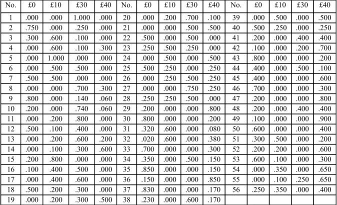
Table 1: The Lotteries
No. £0 £10 £30 £40 No. £0 £10 £30 £40 No. £0 £10 £30 £40 1 .000 .000 1.000 .000 20 .000 .200 .700 .100 39 .000 .500 .000 .500 2 .750 .000 .250 .000 21 .000 .000 .500 .500 40 .500 .250 .000 .250 3 .300 .600 .100 .000 22 .500 .000 .500 .000 41 .200 .000 .400 .400 4 .000 .600 .100 .300 23 .250 .500 .250 .000 42 .100 .000 .200 .700 5 .000 1.000 .000 .000 24 .000 .500 .000 .500 43 .800 .000 .000 .200 6 .000 .500 .500 .000 25 .500 .250 .000 .250 44 .400 .000 .500 .100 7 .500 .500 .000 .000 26 .000 .250 .500 .250 45 .400 .000 .000 .600 8 .000 .000 .700 .300 27 .000 .000 .750 .250 46 .700 .000 .000 .300 9 .800 .000 .140 .060 28 .250 .250 .500 .000 47 .200 .000 .000 .800 10 .200 .000 .740 .060 29 .200 .000 .000 .800 48 .200 .000 .400 .400 11 .000 .200 .800 .000 30 .800 .000 .000 .200 49 .100 .000 .000 .900 12 .500 .100 .400 .000 31 .320 .600 .000 .080 50 .600 .000 .000 .400 13 .000 .200 .600 .200 32 .020 .600 .000 .380 51 .300 .500 .000 .200 14 .000 .100 .300 .600 33 .700 .000 .000 .300 52 .200 .200 .000 .600 15 .200 .800 .000 .000 34 .350 .000 .500 .150 53 .600 .100 .000 .300 16 .100 .400 .500 .000 35 .850 .000 .000 .150 54 .000 .350 .000 .650 17 .000 .400 .600 .000 36 .150 .000 .000 .850 55 .000 .100 .250 .650 18 .500 .200 .300 .000 37 .830 .000 .000 .170 56 .250 .350 .000 .400 19 .000 .200 .300 .500 38 .230 .000 .600 .170
On each of the five occasions the subjects were presented the same 56 lotteries. The lotteries were presented as segmented circles on the computer screen. Figure 1 presents an example in which there is a 50% chance of getting £10, a 20% chance of getting £30, and a 30% chance of getting £40. If a subject received a particular lottery as reward he or she had to spin a wheel on the corresponding circle. The amount won was then determined by the segment of the circle in which the arrow on the wheel stopped.
Figure 1: The Presentation of Lotteries £30
20%
30%
£40 £10 50%
Recall that occasions A and B are irrelevant for the present analysis. In occasions C, D, and E the 56 lotteries appeared in randomized order on screen and subjects were asked for each lottery
• to state their maximal buying price (WTP) in occasion C,
• to state their minimal selling price in occasion D, and
• to state their certainty equivalent under the BDM mechanism in occasion E.
Let us describe the single occasions more detailed now. In occasion C the following question appeared under each lottery: “Submit your bid for this lottery in a second-price sealed-bid auction.” That is subjects were asked to assume they did not have the lottery and had to bid to get it. They had to type in their bid and confirm it by pressing the return key. At the beginning of the experimental session subjects received a three-page instruction sheet. Then an audio-tape of these instructions was played which took approximately ten minutes. The instructions explained clearly the rules and the incentive compatibility of second-price sealed-bid auctions. If a question of occasion C was selected for the reward, the subject received a payment of £y where y is the highest amount in the corresponding lottery. Moreover, if the subject submitted the highest bid among all subjects in the group with whom she completed occasion C, he or she would additionally play out the lottery and had to pay the second highest bid.
Occasion D was identical to occasion C except that for each lottery a different question was asked: “Submit your offer for this lottery in a second-price offer auction”. That is subjects were asked to assume that they owned the lottery and had to make an offer to dispose of it. Again subjects received a handout and had to listen to an audio-tape of the three-page instructions which explained clearly the rules and the incentive compatibility of the second-price offer auction. If a question from occasion D was selected for the reward, the subject could play out the corresponding lottery. However, if he or she submitted the lowest offer among all subjects in the group with whom she completed occasion D, he or she received the second lowest offer instead of the lottery.
In occasion E the following question appeared under each lottery: “State the amount of money such that you do not care whether you will receive this amount or the lottery”. If a question of occasion E was chosen as reward we employed the standard BDM mechanism: A number z was randomly drawn between zero and y where y is the highest possible prize in the given lottery. If z was greater or equal to the answer, the subject received £z, otherwise she or he could play out the given lottery. Also in occasion E subjects received a handout and had to listen to an audio-tape of the instructions which clearly explained the rules and the incentive compatibility of the BDM mechanism.
3. Estimation procedure and preference functionals
Our estimation procedure is similar to the one used by Hey and Orme (1994) which is motivated by two fundamental observations. First, there is not necessarily one best preference functional for all subjects but the behaviour of different subjects may be explained best by different functionals. Second, subjects make from time to time errors in their responses which demands a stochastic specification of preference functionals for our empirical test. To take into account the first observation we have estimated the models subject by subject. To take into account the second observation we have added an error term to each preference functional. We assume that errors are identically and independently distributed among subjects and questions.
For the estimation we extended our set of four outcomes to nine outcomes as follows. Consider for instance lottery 2 of table 1:
No. £0 £10 £30 £40
2 .750 .000 .250 .000
We simply add five additional outcomes, i.e. £5, £15, £20, £25, and £30, to our set of outcomes and present lottery 2 as follows:
No. £0 £5 £10 £15 £20 £25 £30 £35 £40
2 .750 .000 .000 .000 .000 .000 .250 .000 .000
Assume that a particular subject states that her or his certainty equivalent under the BDM mechanism for lottery 2 equal to £10. In this case we can conclude that lottery 2 is strictly preferred to the following two lotteries:
No. £0 £5 £10 £15 £20 £25 £30 £35 £40
a 1.000 .000 .000 .000 .000 .000 .000 .000 .000 b .000 1.000 .000 .000 .000 .000 .000 .000 .000
Moreover, she or he will be obviously indifferent between lottery 2 and the following lottery c:
No. £0 £5 £10 £15 £20 £25 £30 £35 £40
c .000 .000 1.000 .000 .000 .000 .000 .000 .000
And finally he will strictly prefer all the following lotteries to lottery 2:
No. £0 £5 £10 £15 £20 £25 £30 £35 £40
d .000 .000 .000 1.000 .000 .000 .000 .000 .000 e .000 .000 .000 .000 1.000 .000 .000 .000 .000 f .000 .000 .000 .000 .000 1.000 .000 .000 .000
g .000 .000 .000 .000 .000 .000 1.000 .000 .000 h .000 .000 .000 .000 .000 .000 .000 1.000 .000 i .000 .000 .000 .000 .000 .000 .000 .000 1.000
We used this procedure for each lottery in all three occasions. This means that we can derive from our pricing data 504 pairwise preference statements for each subject and each occasion. These preference statements are the data basis for our estimation. More precisely, we used the maximum likelihood method to estimate the parameters of the single preference functionals. The
estimation was performed by a special program we wrote using the GAUSS software package1.
An alternative to our approach would be to use the certainty equivalents directly. If W is the
preference functional and CE(p) the certainty equivalent of lottery p one could simply take the
equation CE = W-1(W(p)) as basis for the estimation.Compared to our method, here the problem
occurs that the stated certainty equivalent will in general lie between two of the outcomes used for the estimation which makes interpolation necessary. To explore the non-trivial problem which of the two estimation techniques is superior we decided to run a Montecarlo simulation.
The simulation technique is as follows: we chose a particular utility function (i.e. u(x) = x1/2) and
calculated the preferences between the lotteries used in our experimental design resulting from this utility function in the expected utility framework. Then we estimated the utility values resulting from these preferences employing both estimation techniques. We call the alternative method “interpolation technique” (IT) why we call our technique “fictitious gamble technique” (FGT). Table 2 reports the findings of the simulation:
Table 2: The Simulation
FGT IT
u(10) u(30) u(10) u(30)
Mean 3.1206 5.5081 3.4500 5.5756
Variance 0.0313 0.0848 0.0030 0.0014
Bias 0.0017 0.0009 0.0828 0.0096
MSE 0.0330 0.0857 0.0858 0.0111
Table 2 reports mean and variance of the estimated utility values for both techniques. The bias of
each estimator is given by the estimated utility value minus the true utility value, i.e. x1/2. It turns
out that IT estimators have a higher bias but a smaller variance. Comparing the mean squared error (MSE) of the two estimators we have to prefer FGT to estimate u(10) and IT to estimate
Now we want to present the preference functionals used in our analysis. Let x = {x1, x2, …, x9} be the extended vector of outcomes as explained above, i.e. (£0, £5, £10, £15, £20, £25, £30, £35, £40). Since we used the certainty equivalents to derive pairwise preference statements our data involve always two lotteries which are represented by two probability vectors denoted by p = {p1, p2, …, p9} and q = {q1, q2, …, q9}. If W denotes the subject’s preference function then V(p,
q) := W(p)-W(q) will be called the relative evaluation. If a particular subject actually does prefer
p to q then her or his net preference function, V(p, q) obviously will be positive. On the other
hand, if she or he actually prefers q to p V(p, q) will be less then zero. Finally, we have V(p, q)
= 0 in the case of indifference.
Altogether subjects’ derived preferences are determined by:
V*(p, q) = V(p, q) + ε ,
where ε is an error term. We assume that ε is symmetric and has a mean of zero.
The first model we have estimated is risk neutrality (RN) given by
RN: V*(p, q) =
∑
= + 9 1 i i ix r k ε .For RN we have to estimate only the parameter k which is the relative magnitude of subjects’
errors. Let us now turn to expected utility (EU) where we have
EU: V*(p, q) =
∑
( )
+ ε = 9 2 i i i x u r .For EU we estimated u(xi), i = 2, 3, 4, 5, 6, 7, 8, 9. We normalized u(x1), i.e. utility of zero, to
zero, and the variance of the error term to one. We did the same also for the three alternative theories presented below. Under this procedure a subject who makes relatively small errors will
have relatively large values for u(xi) whereas a subject who makes relatively large errors will
have relatively small values for u(xi).
The third model is the theory of disappointment aversion (DA) introduced by Gul (1991). The main psychological motivation of this theory is the hypothesis that choice behaviour tries to avoid disappointment where disappointment occurs if the actual outcome of the lottery is lower than the certainty equivalent. In our framework, DA is characterized by the following equation (see also Hey and Orme (1994))
( )
( ) (
)
( )
( ) (
)
( )
ε β β β β + + − + − + − + =∑
∑
∑
∑
∑
∑
− = − = − = − = − = − = = j i i j i i i i j i i j i i j i i i i j i i j q x u q x u q p x u p x u p V DA 8 1 8 2 9 2 8 1 8 2 9 2 8 ,..., 1 , 0 1 1 1 1 min , * : p q .For DA we estimated u(xi), i = 2, 3, 4, 5, 6, 7, 8, 9, and β. The parameter β is Gul’sadditional
parameter which determines the degree of disappointment aversion. If β= 0 DA reduce to EU.
We now turn to rank-dependent utility which is nowadays the most prominent alternative to EU. Note that rank-dependent utility is in our analysis equivalent to cumulative prospect theory since our outcome set does not involve losses. As Hey and Orme (1994) we estimate two variants of rank-dependent utility, one with a power weighting function and one with the weighting function proposed by Quiggin (1982).
For rank-dependence with power function (RP) the weighting function w is given by w(r) = rγ
and we have RP: V*(p, q) =
∑
( )
∑
∑
∑
∑
= = = + = = + + − − − 9 2 9 1 9 9 1 9 j i j i j i i j i i j i i j p p q q x u ε γ γ γ γWe have to estimate u(xi), i = 2, 3, 4, 5, 6, 7, 8, 9, and γ. Note that if γ = 1 RP reduce to EU.
For rank-dependence with ´Quiggin` weighting function (RQ) the weighting function is given by
w(r) = rγ / [rγ + (1 – r)γ]1/γ. This yields RQ: V*(p, q) =
( )
∑
∑
∑
∑
∑
∑
∑
∑
∑
∑
∑
∑
∑
= + = + = + = = = = + = + = + = = = = + − + − − + − − + − − + = 9 2 9 1 1 9 1 9 1 1 9 9 9 1 9 1 9 1 9 1 1 9 9 9 1 1 1 1 j j i i j i i j i i j i i j i i j i i j i i j i i j i i j i i j i i j i i j q q q q q q p p p p p p x u ε γ γ γ γ γ γ γ γ γ γ γ γ γ γ γ γRQ reduces to EU if γ = 1. In the case of RQ we have to estimate u(xi) for i = 2, 3, 4, 5, 6, 7, 8, 9
4. Results
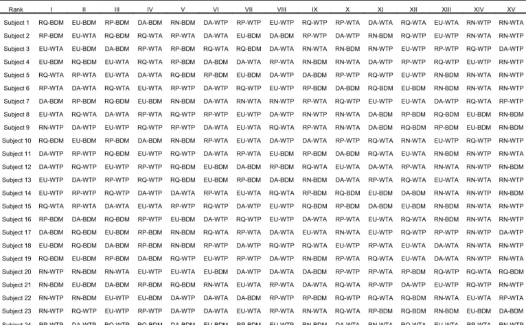
In our analysis we can distinguish 15 different models given by the combination of the five preference functionals with the three different elicitation methods. Table A1 in the appendix is concerned with the question which model represents individual preference best and reports for all of the 24 subjects the precise ranking of the models in terms of their goodness of fit (as measured by the Aikike criterion). Since it is difficult to observe a clear structure in this table it supports the hypothesis that “people are different”. Nevertheless we calculated the average
rankings2 of all 15 models in order to evaluate their performance. Table 3 lists the single models
ordered according to increasing average rank. The first conclusion which emerges from this table is the fact that BDM performs rather well since the models on the first three ranks are all based on BDM. Secondly, it seems to be obvious that RN has a rather poor performance since all models with RN are on the last ranks. The third and possibly the most important conclusion from table 3 is the fact that the performance of a preference functional depends crucially on the employed elicitation method. RQ is for instance, as for choice data analyzed in the study of Hey and Orme (1994), the best preference functional in terms of average rank. However, in the present study this is only true if RQ is combined with BDM. In contrast, combined with WTP or WTA, RQ turns out to be the worst model apart from RN. This clearly shows that there does not exist one “best” preference functional for all tasks but instead for different tasks different preference functional perform better. The last conclusion from table 3 which is also in line with the results of Hey and Orme (1994) is the fact that EU does not seem to perform substantially worse than the alternative preference functionals.
Table 3: Average ranks of the single models
RQ RP EU DA DA RP DA EU EU RP RQ RQ RN RN RN BDM BDM BDM WTP BDM WTP WTA WTP WTA WTA WTP WTA BDM WTA WTP
6,083 6,125 6,292 6,417 6,833 7,167 7,542 7,667 7,875 7,917 8,042 8,375 9,375 11,625 12,125
Since the performance of the single preference functionals depends on the employed elicitation method we analyzed in tables 4-6 each elicitation method separately. More precisely, table 4 lists for each preference functional the number of subjects for whom this preference functional is on the first, second, third, fourth, and last rank in terms of fit for WTP. The last row reports the average rank of each preference functional. Tables 5 and 6 contain the same information for WTA and BDM, respectively.
2 When we calculated the average rankings two models got the same rank if they performed identical. If for example two models have the highest Aikike criterion they both get the first rank and the next model gets rank three. For this reason the average of the average ranks may differ from the rank average.
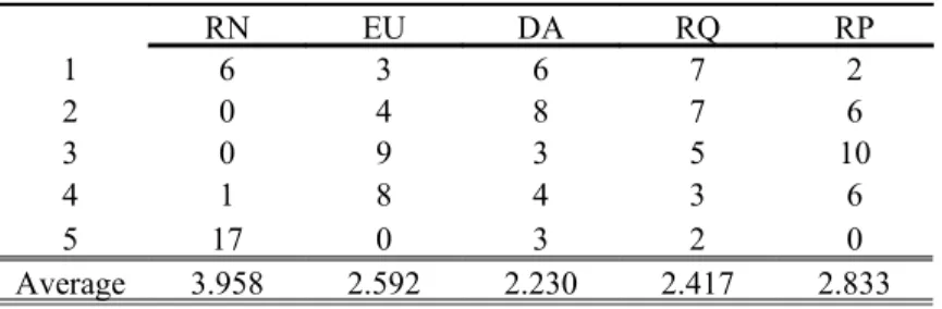
Tables 4-6 show that RN is for all elicitation methods the worst preference functional in terms of average ranks. For WTP and WTA DA turns out to be best while it performs rather poorly under BDM where RP turns out to be best. Since in DA a reference point plays a prominent role the bad performance of DA under BDM may possibly due to the fact that the reference point receives less attention under BDM as compared to WTP and WTA.
Table 4: Ranking of the preference functionals under WTP
WTP RN EU DA RQ RP 1 6 3 6 7 2 2 0 4 8 7 6 3 0 9 3 5 10 4 1 8 4 3 6 5 17 0 3 2 0 Average 3.958 2.592 2.230 2.417 2.833
Table 5: Ranking of the preference functionals under WTA
WTA RN EU DA RQ RP 1 2 4 9 4 6 2 2 6 2 9 5 3 1 5 7 5 7 4 1 9 6 4 3 5 18 0 0 2 3 Average 4.292 2.792 2.417 2.625 2.667
Table 6: Ranking of the preference functionals under BDM
BDM RN EU DA RQ RP 1 3 3 4 6 10 2 0 8 4 5 8 3 1 6 7 9 6 4 0 7 8 4 0 5 20 0 1 0 0 Average 4.417 2.708 2.917 2.458 1.833
The fact that RP is the best preference functional under BDM but performs rather poorly under WTP reinforces our conclusion from above that the performance of the single preference functionals depends crucially on the elicitation method. Altogether, tables 4-6 also show that EU does not perform substantially worse than its alternatives.
Finally we are interested in the question which elicitation method is best for the single preference functionals. Corresponding information is provided in tables 7-11. For instance table 7 reports for each elicitation method the number of subjects for which this elicitation method is best, second best, and worst for RN. Tables 8-11 contain the same information for EU, DA, RQ, and RP respectively.
Table 7: Ranking of the elicitation methods under RN
RN WTP WTA BDM 1 5 3 19 2 4 17 0 3 15 4 5 Average 2.417 2.042 1.417
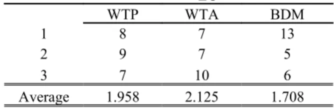
Table 8: Ranking of the elicitation methods under EU
EU WTP WTA BDM 1 8 7 13 2 9 7 5 3 7 10 6 Average 1.958 2.125 1.708
Table 9: Ranking of the elicitation methods under DA
DA WTP WTA BDM 1 9 7 12 2 9 9 4 3 6 8 8 Average 1.875 2.042 1.833
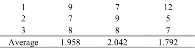
Table 10: Ranking of the elicitation methods under RQ
RQ
1 9 7 12
2 7 9 5
3 8 8 7
Average 1.958 2.042 1.792
Table 11: Ranking of the elicitation methods under RP
RP WTP WTA BDM 1 8 6 13 2 9 9 5 3 7 9 6 Average 1.958 2.125 1.958
It turns out that BDM is always the best elicitation method both in terms of average rank and in terms of number of subjects for which a given elicitation method is best. Additionally, according to these two criteria, WTP is except for RN always better than WTA. The latter result may have some conclusions for the contingent valuation method. Until now it is an open question whether contingent valuation surveys should rely on WTP or WTA. Some authors have argued in favor of WTP since WTA usually decreases during experiments whereas WTP remains relatively constant during the single rounds. Our results seem to provide additional support for WTP.
5 Conclusions
In this paper we have analyzed the empirical performance of several preference functionals. The main difference with existing studies in the literature is the fact that we used pricing data instead of choice data. Our main results can be summarized as follows:
• The performance of the single preference functionals depends crucially on the elicitation
method.
• EU does not perform substantially worse than its alternatives
• DA turns out to be the best preference functional under WTP and WTA while RP is best
under BDM.
• BDM seems to be the best elicitation method and WTA the worst.
Acknowledgements
The experiment was conducted while the second author was visiting EXEC at the University of York. Financial support for this visit by the Deutsche Forschungsgemeinschaft under contracts Schm1396/1-1 and 1-2 is gratefully acknowledged. Financial support for running
the experiment and for the payment of the subjects was obtained from the TMR ENDEAR project of the European Union under contract CT98-0238. The paper was written during a visit of the second author at the University of Bari. Financial support for this visit was provided by the Danish Social Science Research Council under contract 24-02-0128. First of all we have to thank John D. Hey for his advice and guidance concerning the experimental design and the analysis performed in this paper. We are indebted to Norman Spivey for writing the software for this experiment. Also thanks to Stefan Traub for help with the data processing. For critical and helpful comments on the instructions we have to thank Marie Edith Bissey, Carmela DiMauro, and Anna Maffioletti. Useful comments on the current version of the paper were given by Han Bleichrodt.
References
Allais, M. (1953), “Le Comportement de l'Homme Rationnel devant le Risque, Critique des
Postulates et Axiomes de l'Ecole Américaine”, Econometrica 21, 503-546.
Becker, G.M., DeGroot, M.E. and Marschak, J. (1963), “An Experimental Study of Some
Stochastic Models for Wagers”, Behavioral Science 8, 199-202.
Carbone, E. and Hey J. D. (1994) “Estimation of Expected Utility and Non-Expected Utility Preference Functionals Using Complete Ranking Data”, In B. Munier and M.J. Machina
(eds.), Models and Experiments on Risk and Rationality, Kluwer, Boston, 119-39.
Carbone, E. and Hey J. D. (1995) “A Comparison of the Estimates of EU and non-EU Preference Functionals Using Data from Pairwise Choice and Complete Ranking
Experiments”, GenevaPapers on Risk and Insurance Theory 20, 111-133.
Gul, F. (1991), “A Theory of Disappointment Aversion”, Econometrica 59, 667-686.
Harless, D.W. and Camerer, C.F.(1994), “The Predictive Utility of Generalized Expected
Utility Theories”, Econometrica 62, 1251-1289.
Hey, J.D., and Orme, C. (1994), Investigating Generalizations of Expected Utility Theory
Using Experimental Data, Econometrica 62, 1291-1326.
Knetsch, J.L., and Sinden, J.A. (1984), “Willingness to Pay and Compensation Demanded:
Experimental Evidence of an Unexpected Disparity in Measures of Value”, Quarterly
Journal of Economics 99, 507-521
Lichtenstein, S., and Slovic, P. (1971), “Reversals of Preferences Between Bids and Choices
in Gambling Decisions”, Journal of Experimental Psychology 89, 46-55.
Quiggin, J. (1982), “A Theory of Anticipated Utility”, Journal of Economic Behavior and
Organization 3, 323-343.
Schmidt, U. (2002), “Alternatives to Expected Utility: Some Formal Theories”, in: P.J.
Hammond, S. Barberá, and C. Seidl (eds.), Handbook of Utility Theory Vol. II, Kluwer,
Boston, forthcoming.
Starmer, C. (2000), “Developments in Non-Expected Utility Theory : The Hunt for a
Descriptive Theory of Choice under Risk”, Journal of Economic Literature 38, 332-382.
Sugden, R. (2002), “Alternatives to Expected Utility: Foundations”, in: P.J. Hammond, S.
Barberá, and C. Seidl (eds.), Handbook of Utility Theory Vol. II, Kluwer, Boston,
forthcoming.
von Neumann, J. and Morgenstern, O. (1944), Theory of Games and Economic Behavior,
Appendix
Rank I II III IV V VI VII VIII IX X XI XII XIII XIV XV
Subject 1 RQ-BDM EU-BDM RP-BDM DA-BDM RN-BDM DA-WTP RP-WTP EU-WTP RQ-WTP RP-WTA DA-WTA RQ-WTA EU-WTA RN-WTP RN-WTA Subject 2 RP-BDM EU-WTA RQ-BDM RQ-WTA RP-WTA DA-WTA EU-BDM DA-BDM RP-WTP DA-WTP RN-BDM RQ-WTP EU-WTP RN-WTA RN-WTP Subject 3 EU-WTA EU-BDM DA-BDM RP-WTA RP-BDM RQ-WTA RQ-BDM DA-WTA RN-WTA RN-BDM RN-WTP EU-WTP RP-WTP RQ-WTP DA-WTP Subject 4 EU-BDM RQ-BDM EU-WTA RQ-WTA RP-BDM DA-BDM DA-WTA RP-WTA RN-BDM RN-WTA DA-WTP RP-WTP RQ-WTP EU-WTP RN-WTP Subject 5 RQ-WTA RP-WTA EU-WTA DA-WTA RQ-BDM RP-BDM EU-BDM DA-WTP DA-BDM RP-WTP RQ-WTP EU-WTP RN-BDM RN-WTA RN-WTP Subject 6 RP-WTA DA-WTA RQ-WTA EU-WTA RP-WTP DA-WTP RQ-WTP EU-WTP RP-BDM DA-BDM RQ-BDM EU-BDM RN-BDM RN-WTA RN-WTP Subject 7 DA-BDM RP-BDM RQ-BDM EU-BDM RN-BDM DA-WTA RN-WTA RN-WTP RP-WTA RQ-WTP EU-WTP EU-WTA DA-WTP RQ-WTA RP-WTP Subject 8 EU-WTA RQ-WTA DA-WTA RP-WTA RQ-WTP RP-WTP EU-WTP DA-WTP RN-WTP RN-WTA DA-BDM RP-BDM RQ-BDM EU-BDM RN-BDM Subject 9 RN-WTP DA-WTP EU-WTP RQ-WTP RP-WTP DA-WTA EU-WTA RQ-WTA RP-WTA RN-WTA DA-BDM RQ-BDM RP-BDM EU-BDM RN-BDM Subject 10 RQ-BDM EU-BDM RP-BDM DA-BDM RN-BDM RP-WTA EU-WTA DA-WTP DA-WTA RP-WTP RQ-WTA RN-WTA EU-WTP RQ-WTP RN-WTP Subject 11 DA-WTP RP-WTP RQ-BDM EU-WTP RQ-WTP DA-WTA RP-WTA EU-BDM RP-BDM DA-BDM RQ-WTA EU-WTA RN-BDM RN-WTP RN-WTA Subject 12 DA-WTP RQ-WTP EU-WTP RP-WTP RQ-BDM EU-BDM DA-BDM RP-BDM RQ-WTA EU-WTA DA-WTA RP-WTA RN-WTA RN-WTP RN-BDM Subject 13 EU-WTP DA-WTP RP-WTP RQ-WTP RQ-BDM EU-BDM RP-BDM DA-BDM RN-BDM DA-WTA RP-WTA RQ-WTA EU-WTA RN-WTA RN-WTP Subject 14 EU-WTP RP-WTP RQ-WTP DA-WTP DA-WTA RP-WTA EU-WTA RQ-WTA RP-BDM RQ-BDM EU-BDM DA-BDM RN-WTA RN-WTP RN-BDM Subject 15 RQ-WTA RP-WTA DA-WTA EU-WTA RP-WTP RQ-WTP DA-WTP EU-WTP RQ-BDM RP-BDM DA-BDM EU-BDM RN-BDM RN-WTA RN-WTP Subject 16 RP-BDM DA-BDM RQ-BDM RP-WTP EU-BDM DA-WTP RQ-WTP EU-WTP DA-WTA RP-WTA EU-WTA RQ-WTA RN-BDM RN-WTA RN-WTP Subject 17 DA-BDM RQ-BDM EU-BDM RP-BDM RN-BDM RQ-WTA RP-WTA DA-WTA EU-WTA RN-WTA EU-WTP RQ-WTP RP-WTP RN-WTP DA-WTP Subject 18 EU-BDM RQ-BDM DA-BDM RP-BDM RN-BDM RP-WTP DA-WTP RQ-WTP RQ-WTA EU-WTP RP-WTA EU-WTA DA-WTA RN-WTA RN-WTP Subject 19 RQ-BDM EU-BDM RP-BDM DA-BDM RQ-WTP EU-WTP RP-WTP DA-WTP RN-BDM RP-WTA RQ-WTA EU-WTA DA-WTA RN-WTP RN-WTA Subject 20 RN-WTP RN-BDM RN-WTA EU-WTP EU-WTA EU-BDM DA-WTP DA-WTA DA-BDM RP-WTP RP-WTA RP-BDM RQ-WTP RQ-WTA RQ-BDM Subject 21 RN-BDM EU-BDM DA-BDM RP-BDM RQ-BDM RN-WTA EU-WTA RP-WTA DA-WTA RQ-WTA RP-WTP DA-WTP EU-WTP RQ-WTP RN-WTP Subject 22 RN-WTP RN-BDM EU-WTP EU-BDM DA-WTP DA-WTA DA-BDM RP-WTP RP-BDM RQ-WTP RQ-WTA RQ-BDM RN-WTA EU-WTA RP-WTA Subject 23 RN-WTP RQ-WTP EU-WTP RP-WTP DA-WTP DA-WTA EU-WTA RP-WTA RN-WTA RQ-WTA RP-BDM RQ-BDM RN-BDM EU-BDM DA-BDM Subject 24 RP-WTP DA-WTP RQ-WTP RQ-BDM DA-BDM EU-BDM RP-BDM EU-WTP RN-BDM DA-WTA RN-WTA RQ-WTA EU-WTA RP-WTA RN-WTP