LEARNING COLOUR CONSTANCY USING CONVOLUTIONAL
NEURAL NETWORKS
Master of Science thesis
Examiner: Prof. Moncef Gabbouj, Jari Niemi
Examiner and topic approved by the Faculty Council of the Faculty of Computing and Electrical Engineering on 12th August 2015
i
ABSTRACT
HIDIR YÜZÜGÜZEL: Learning Colour Constancy Using Convolutional Neural Networks
Tampere University of Technology
Master of Science thesis, 45pages, 0Appendix pages November 2015
Master's Degree Programme in Information Technology Major: Signal Processing
Examiner: Prof. Moncef Gabbouj, Jari Niemi
Keywords: colour constancy, machine learning, deep learning, convolutional neural net-work
Colour constancy has attracted attention of researchers from the academy and indus-try as it is a fundamental preprocessing task in many computer vision applications. Colour constancy is a feature of human visual system which enables humans to perceive colors of the objects invariant to the illuminant. However, it has been a challenging problem for computers due to its ill-posed structure.
Articial neural networks have recently been very popular due to breakthrough results of deep neural networks in recognition tasks. Deep neural networks learn hierarchical representations (features) of data, which has started a new era in ma-chine learning eld. Deep neural network models combine the feature learning and regression as a complete optimization procedure, namely they are an end-to-end learning approach.
In this thesis, we investigate learning colour constancy using deep convolutional neu-ral (CNN) networks. Unlike traditional color constancy methods, CNN model does not rely on any explicit imaging assumptions and hand-crafted features. Two dier-ent CNN models are trained and evaluated on two widely used datasets (Shi-Gehler and SFU subset) from scratch. The results are compared with traditional statistics based approaches. It has been justied that CNN model signicantly outperforms statistics based methods on both datasets. The improvements in average angular error are 26.6% and 20% for Shi-Gehler and SFU subset respectively.
PREFACE
This thesis has been conducted in the Department of Signal Processing, Tampere University of Technology.
I would like to thank to my supervisor Academy Professor Moncef Gabbouj for all his support throughout the course of this research. I also would like to thank to my examiner, Jari Niemi for the valuable feedback he has provided for this thesis. It has been a great pleasure for me to have an examiner and a friend at the same time. I would like to thank to the members of the Multimedia Research Group (MUVIS) for their friendship. Particularly, many thanks go to Prof. Serkan Kiranyaz for providing me the opportunity to join MUVIS team. It is not possible to mention everyone here, but I would not forget Berkay Kicananaoglu for fruitful discussions and coee breaks.
Hdr Yüzügüzel
iii
TABLE OF CONTENTS
1. Introduction . . . 1 2. Theoretical Background . . . 4 2.1 Machine Learning . . . 4 2.2 Colour Constancy . . . 62.2.1 Image formation model . . . 6
2.2.2 Statistics based approaches . . . 7
2.2.3 Learning based approaches . . . 8
2.3 Articial Neural Networks . . . 10
2.3.1 Perceptron . . . 10
2.3.2 Multilayer perceptron . . . 11
2.3.3 Autoencoder (Autoassociator) . . . 13
2.3.4 Training ANN . . . 14
2.3.5 Regularization . . . 19
2.4 Deep Convolutional Neural Network . . . 21
2.4.1 Convolution . . . 22
2.4.2 Pooling (Subsampling) . . . 24
2.4.3 Rectied Linear Unit (ReLU) . . . 25
3. Methodology . . . 26
3.1 Preprocessing . . . 26
3.1.1 Gamma correction . . . 26
3.1.2 Image resizing and cropping . . . 26
3.1.3 Non-overlapping patch extraction . . . 27
3.1.4 Global histogram stretching . . . 27
3.1.5 Feature standardization . . . 28
3.3 CNN training and testing . . . 30
4. Experimental setup and results . . . 31
4.1 Datasets . . . 31
4.2 Error Measure . . . 32
4.3 Results . . . 33
5. Conclusions . . . 41
v
LIST OF FIGURES
1.1 Correct white balance vs. reddish/yellowish white balance (Source: http://www.cs.mtu.edu/~shene/DigiCam/User-Guide/white-balance/
wb-concept.html) . . . 2
2.1 rg chromaticity spaces of images in Figure 1.1 . . . 9
2.2 Sigmoid and tanh activation functions . . . 11
2.3 Simple perceptron . . . 12
2.4 One-hidden-layer toy MLP with D= 3, K = 2, Dh = 5 . . . 12
2.5 Autoencoder example (LayerL2 acts as an encoder and layerL3 acts as a decoder) . . . 14
2.6 Learned colour features on STL-10dataset with a sparse autoencoder 15 2.7 Learned hierarchical features from a DL algorithm [20] . . . 22
2.8 An example of2D convolution without kernel ipping (Source: http: //www.iro.umontreal.ca/~bengioy/dlbook/version-07-08-2015/ convnets.html) . . . 24
2.9 Illustration for sparse connectivity and weight sharing (Source: http: //deeplearning.net/) . . . 24
3.1 Plots of Equation 3.1 for various values of γ (c= 1 in all cases) . . . 27
3.2 CNN architecture . . . 29
4.1 Example images of Shi-Gehler RAW dataset . . . 32
4.2 Example images of SFU subset dataset . . . 32
4.4 Worst mean pooling CNN result in Shi-Gehler . . . 36
4.5 Best median pooling CNN result in Shi-Gehler . . . 37
4.6 Worst median pooling CNN result in Shi-Gehler . . . 38
4.7 Best mean pooling CNN result in SFU subset . . . 39
4.8 Worst mean pooling CNN result in SFU subset . . . 39
4.9 Best median pooling CNN result in SFU subset . . . 40
vii
LIST OF TABLES
2.1 Statistics based colour constancy algorithms . . . 8 3.1 Parameters in CNN training . . . 30 4.1 Angular error statistics on linear Shi-Gehler RAW dataset . . . 34 4.2 Angular error statistics on linear Gray-ball (SFU) subset dataset . . . 34
LIST OF ABBREVIATIONS AND SYMBOLS
AE Automatic exposure, page1AF Automatic focus, page 1
ANN Articial Neural Network, page 4 AWB Automatic White Balance, page 1 BP Backpropagation, page 13
CC Colour Constancy, page 1
CNN Convolutional Neural Network, page 3
DL Deep Learning, page 3
GPU Graphical Processing Unit, page 21 MLP Multilayer Perceptron, page 4 ReLU Rectied Linear Unit, page 22 SVM Support Vector Machine, page4 SVR Support Vector Regression, page8
b b chromaticity value, page 9
b(1) bias vector of rst hidden layer in MLP, page 13
b(2) bias vector of second hidden layer in MLP, page 13
B blue value of colour image pixel, page 2
c camera sensor spectral sensitivity, page 6
D input feature dimension, page 10
Dh dimension of hidden layer neurons, page 12
e colour of light source, page 2 ˆ
e estimated colour of light source, page 33 exp exponential function, page 11
E error, page 5
E0 augmented error, page 19
g g chromaticity value, page 8
g(.) model, page 5
G green value of colour image pixel, page 2 Gσ gaussian lter, page 7
i, j, h indices, page6
I (sub)image function, page6
ix
K output dimension in ANN, page 11
K number of cross validation folds, page 5 L(.) loss function, page 5
n order of derivative, page 7
N total number of samples, page 4
p Minkowski norm, page 7
P model complexity function, page 19
r desired output response (label), page 4
r r chromaticity value , page 8
r∗ desired output for (unseen) test input feature/pattern vector, page
4
R red value of colour image pixel, page 2
s surface reectance, page 6
t sample index, page 4
vih connection weight between ith unit in output layer and hth unit in
hidden layer, page 18
V weight matrix between hidden and output layer in MLP, page 13
w weight vector, page 10
w0 intercept value of ANN, page 10
whj connection weight between jth unit in input layer and hth unit in
hidden layer, page 17
wj jth element of weight vector, page 10
W weight matrix between input and hidden layer in MLP, page 13
x input feature/pattern vector, page 4 ¯
x mean of x, page28
x∗ (unseen) test input feature/pattern vector, page 4
x0 bias unit in ANN, page 10
xj jth feature of input feature/pattern vector, page 10
X training set, page 4
y (predicted) output vector, page 10
yi ith unit of (predicted) output vector, page 17
z output of hidden layer neurons, page 13
α momentum parameter, page 19
∆ change of any changeable quantity, page 16
η learning rate, page 16
γ gamma, page 26
∇ gradient, page 7
ψ regularization parameter, page 19
σ scale parameter (standard deviation), page 7
θ parameters, page 5
θ∗ best parameters, page 5
ϕ ANN activation function, page13
∂E
∂θ gradient of error function, page 13
k.k norm, page 21
1
1. INTRODUCTION
Computer vision is the term that denes a multidisciplinary research eld which aims to acquire, process, analyze and understand images. The elds most closely related to computer vision are image processing, pattern recognition, signal processing and machine learning. The computer vision problems can be mainly divided into two groups such as high level and low level vision tasks. Subelds of high level computer vision include object recognition, object tracking, image classication and so on. Among many subelds of low level computer vision (such as noise reduction, tone mapping, auto-focus, auto-exposure etc.), colour constancy (CC) remains to be a challenging problem due to its ill-posed nature.
CC is the ability to measure colours of objects independently of the colour of the light source [25]. CC is also known as (automatic) white balance, colour balance, gray balance and white point estimation problem in the literature. Generally speaking, Human Visual System can perceive the colours of the objects, despite the variations in ambient illuminant. A correctly and badly white balanced image pair is shown in Figure 1.1. In contrast, CC is not a trivial task for the computers. A great deal of research has been conducted into CC problem.
CC is a fundamental pre-processing step for various high level computer vision tasks. Besides, it is one of the three key problems (auto-focus, auto-exposure, auto-white-balance) in digital camera pipeline. In general, these three problems are referred together to as "3A's": AF/AE/AWB. Therefore, it is important for the end-users of the digital cameras and mobile phones who want to take aesthetically plausible images with their devices.
Traditional computational CC models attack the problem using a two step proce-dure, namely illuminant estimation and colour correction. Firstly, they estimate the colour (chromaticity) of the light source (illuminant) from a RGB input image based on some assumptions. The most common assumption is uniform light source colour across the scene. Secondly, they correct the input image using that estimated
illuminant so that the corrected image appears to be taken under a canonical, e.g. perfect white (i.e.
1/√3, 1/√3, 1/√3T), light source [1]. The colour correction is achieved by inverting a diagonal model named Von-Kries Model:
R G B = eR 0 0 0 eG 0 0 0 eB R0 G0 B0 (1.1)
where [R G B]T is the colour of any pixel taken under an unknown light source,
R0 G0 B0T is the transformed colour which would appear as if it were under
canon-ical light source and [eR eG eB]T is the colour of the light source which has already
been estimated in the rst step. As can be seen from Equation 1.1, the second step of the procedure is straightforward when the illuminant is estimated accurately.
Figure 1.1 Correct white balance vs. reddish/yellowish white balance (Source: http: // www. cs. mtu. edu/ ~shene/ DigiCam/ User-Guide/ white-balance/ wb-concept. html )
Many illumination estimation algorithms have been presented in the literature. The proposed solutions for CC can be roughly classied into two main groups: statistics-based vs. learning-statistics-based approaches. The former type of algorithms are methods which are directly applied to any image without requiring training. For the lat-ter type of algorithms, a model should be learnt before the illumination can be estimated.
1. Introduction 3 Traditional machine learning techniques require careful hand-crafted feature engi-neering as the performance of machine learning methods depends on the data repre-sentation (or features). In other words, one should have domain expertise to design a feature extractor which transforms the raw data, e.g. pixel values of an image, into a suitable internal representation (feature vector). Another important drawback of feature engineering is that features extracted from one dataset do not work well on another dataset. These diculties of feature engineering motivated researcher to nd out algorithms to learn features. In deep learning (DL) models features are not designed by humans but they are automatically learned from the raw data for the task at hand. Contrary to feature engineering approach, there is no need to design features manually ahead of time.
In this thesis, a deep convolutional neural network (CNN) model is trained to esti-mate the colour of the light source from the non-overlapping patches extracted from the almost raw input colour images. Although CNNs are proved to be extremely successful in high level vision tasks, such as recognition, using CNNs for low level vision tasks, such as CC, is a quite new idea and, to our knowledge, [8] is the only work that investiages the use of CNNs for illumination estimation. As opposed to [8], which trains and evaluates the CNN on a single dataset, we train and evaluate two dierent CNN models from scratch on two dierent widely used datasets. Fur-ther, our CNN model yields similar performance as [8] by extracting fewer patches in an intelligent way on Shi-Gehler dataset. Our simple patch extraction strategy signicantly reduces the computational burden compared to [8].
The rest of the thesis is organized as follows. In Chapter 2, we formulate the CC problem and present a short literature review on CC. In this chapter, we also provide the necessary background information. In Chapter 3, we present the pre-processing and our CNN model in detail. In Chapter 4, we present our experimental results. Finally, Chapter 5 oers concluding remarks.
2. THEORETICAL BACKGROUND
This chapter starts with a brief overview on machine learning paradigm. Then, existing CC methods will be discussed. Further, articial neural network (ANN) models are presented. Finally, a deep CNN model is described.
2.1 Machine Learning
Machine learning refers to computer programs which can improve their performance
P in some task(s) T by their own experience E [21]. There is a model dened
up to some parameters, and learning refers to optimization of the parameters of the model using training data or past experience. Most often, machine learning is used interchangeably with the term Pattern Recognition (PR) although they are not exactly the same.
There are two main subelds of machine learning, namely, supervised learning and unsupervised learning. In supervised learning, there exists a training set X = {xt, rt}N
t=1 where x is the feature/pattern vector, r is the desired output (usually called as label, particularly in the context of classication), t is the index of
dier-ent samples in the set ofN samples. The aim is to learn a mapping from the inputx
to an outputr such that given a novel inputx∗ the predicted outputr∗ is accurate.
The pair (x∗, r∗) is not in X but assumed to be generated by the same unknown process that generated X. The term 'supervised' indicates that there is a so-called 'supervisor' who provides the output r for each input x in the training data X. There exist many supervised learning techniques in the literature: k-nearest neigh-bour (kNN), multilayer perceptron (MLP), decision tree, support vector machine (SVM) and so on. Unlike supervised learning, in unsupervised learning, there is no supervisor and we have only the input data x, i.e. we do not have output values r.
The aim is to nd interesting and hidden structure in the unlabelled input data. It is closely related to density estimation in statistics. Among many other techniques such as matrix factorization, clustering methods are most widely used unsupervised
2.1. Machine Learning 5 learning methods.
Supervised learning has two important applications, namely classication and re-gression. Classication deals with the prediction of categorical class labels whereas regression models continuous-valued functions. An example application for classi-cation would be e.g. classifying images of humans as 'male' or 'female'. A regression example would be e.g. predicting the price of a used car. The regular approach in machine learning [6] is that we assume a model g(x|θ) where g(.) is the model, x
is the input and θ are the parameters. The machine learning program optimizes
the parameters θ such that the approximation error, or loss, is minimized. The
approximation error E is the sum of individual losses over the instances of X:
E(θ|X) =X
t
L(rt−g(xt|θ)) (2.1) whereL(.)is the loss of the residual between the desired outputrt and our
approx-imation to it g(xt|θ) given the current value of the parameters θ. We aim to nd
best parameters θ∗ that minimize the total error:
θ∗ = arg min
θ E(θ|X) (2.2)
After training phase is completed, i.e. parametersθ∗ are found, we are interested in
the generalization performance (o-training set error) of the learning algorithm. Per-formance assessment is an essential part of machine learning system. PerPer-formance evaluation methods can be grouped into three categories, namely resubstituation error rate, holdout error rate and cross validation error rate. The simplest error rate estimate is the resubstituation error rate which is the training error rate. It is an optimistic estimate of the machine learning system. For example, the training error of 1-nearest neighbour is always zero. In holdout case, we split the dataset into two dierent sets: training and test set. This division is usually performed after the dataset is randomly shued. Holdout method is not suitable for small datasets since there will not be adequate training data to train the learning algorithm after splitting. In this situation, a better method is cross-validation, in which the dataset is divided into K equal sized parts (folds) and one of the K parts is used as test
set, while remaining K −1 parts are used as training set. This training/testing is repeated K times and an average of test errors on each fold is calculated as test
error estimate. Cross-validation is also referred to as K-fold cross validation. In the
extreme case where K =N, it is named as leave-one-out method. Leave-one-out is
quite useful when there the datasets are very small.
2.2 Colour Constancy
2.2.1 Image formation model
CC is an under-determined (ill-posed) problem since we have one image and two unknowns (illuminant and reectance). The basic image formation model is quite handy to understand the ill-posedness. We shall denote images by two-dimensional functions of the form I(i, j). The function I(i, j) is mainly characterized by two components [16]:
• the amount of source illumination incident on the scene being viewed (illumi-nation)
• the amount of illumination reected by the objects in the scene (reectance) If we want to write the image formation model more rigorously,
I(i, j) = Z
e(i, j, λ)s(i, j, λ)c(λ)dλ (2.3)
where
• λ: wavelength of the illuminant
• I(i,j): intensity value of the pixel at given position (i,j)
• e(i,j,λ): illuminant spectral power distribution
• s(i,j,λ): surface spectral reactance
• c(λ): sensor spectral sensitivities (0≤c(λ)≤1)
CC problem tries to solve botheand sgiven oneI andc, which makes the problem
2.2. Colour Constancy 7
2.2.2 Statistics based approaches
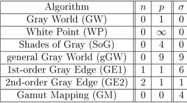
To tackle the ill-posedness problem additional assumptions are needed. The statis-tics based methods are based on assumptions about the distribution of colours in the image. The most common and widely used instance of this class is Gray World [9] assumption. It is assumed that average colour in the image is gray and therefore, the illuminant colour can be estimated as a deviation from gray of the averages in image colour channels. Another well-known instance of this class is White Patch [19] assumption. It is assumed that there always exists a white patch in the im-age and the maximum response in each channel is caused by perfect reection of the illuminant on the white patch. As a result of this, the colour of this perfect reectance is exactly the colour of the light source. A third instance of this class is Gray Edge [25] assumption in which higher order image statistics, namely image derivatives, are utilized. It is assumed that average colour of the edges are gray and the illuminant colour can be estimated as the deviation from gray of the averages of the edges in the image colour channels. Van der Weijeer et. al. combined all these statistics based methods into a single framework (Equation 2.4) of CC methods based on low level image features [25].
e(n, p, σ) = 1 k Z Z |∇nI σ(i, j)|pdxdy 1p (2.4) where
• n: order of the derivative
• p: order of the Minkowski norm
• Iσ(i, j) = I(i, j)∗Gσ(i, j)whereGσ(i, j)is a gaussian lter with scale parameter
σ
• k: constant such that illuminant colour e has unit length (using L2 norm) By varying n, pand σ, we result in dierent statistics based CC algorithms (Table
2.1).
The statistics based methods are considered as state-of-the-art and are widely in use. The drawback of statistics based approaches is that they only work well when some
Algorithm n p σ
Gray World (GW) 0 1 0
White Point (WP) 0 ∞ 0
Shades of Gray (SoG) 0 4 0 general Gray World (gGW) 0 9 9 1st-order Gray Edge (GE1) 1 1 6 2nd-order Gray Edge (GE2) 2 1 1
Gamut Mapping (GM) 0 0 4
Table 2.1 Statistics based colour constancy algorithms
pre-dened assumptions are satised. For example, gray world assumption does not hold for every image since the average intensity of primary colours is assumed to be equal. As an example, when taking photos of a forest, it is obvious that the average intensity of the green channel diers from averages of red and blue. On the other hand, the main advantage of statistics based approaches is that they require very low computational resources. For example, white patch (max-RGB) nds the maximum or gray world computes average pixel values.
2.2.3 Learning based approaches
The learning based CC algorithms estimate the colour of the light source using a model that is learnt in a supervised manner, in which we have labelled training data. Learning CC can be formulated as a regression problem. Although any machine learning technique can be used for regression, in the literature mostly MLP [10], support vector regression (SVR) [12] and ridge regression [5] are used. The pro-posed learning based methods usually rely on hand-crafted low level visual features such as pixels. Mostly, as input (feature) representation, binarized rg chromaticity
histogram of the images are used and the measured ground truth illuminations are given as desired output in learning based approaches. rg chromaticity space:
r=R/(R+G+B) (2.5)
g =G/(R+G+B) (2.6)
where RGB refers to red, green and blue. rgchromaticity space is bounded between
2.2. Colour Constancy 9 being an input to a learner. It is important to note that usingrg chromaticity space
discards all spatial and intensity information, which has pros and cons [10]. Therg
chromaticity space is uniformly quantized with a xed step size. The binary input (feature) representation is constructed by binarizing the quantized rg chromaticity
space.
Figure 2.1 rg chromaticity spaces of images in Figure 1.1
When the blue chromaticity component is necessary, it can easily be calculated:
b = 1−r−g (2.7)
There also exist dierent chromaticity spaces, such as:
r=R/G (2.8)
b =B/G (2.9)
MLP will be discussed in more detail in Chapter 2.3.2. SVR, which is also referred to as a kernel machine, is a maximum margin method that allows the model to be written as a sum of the inuences of a subset of the training instances, namely so-called support vectors [6]. Both MLP and SVR are nonlinear regression methods.
Ridge regression is an extension to linear regression which incorporates regulariza-tion. In linear regression, the sum of squared errors are minimized whereas in ridge regression, combination of both sum of squared errors and the norm of coecient vector is minimized.
Bayesian approaches [13] model the variability of reectance and of illuminant as random variables, and then estimate illuminant from posterior probability distribu-tion condidistribu-tioned on image data.
2.3 Articial Neural Networks
2.3.1 Perceptron
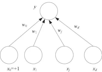
The perceptron is the elementary processing unit in ANN models. It has inputs
xj ∈ R, j = 1, . . . , D, associated weights wj ∈ R and output y. The weights are
often named as synaptic weight or connection weight. In the simplest form, it is a weighted sum of its inputs (Figure 2.3):
y=
D
X
j=1
wjxj +w0 (2.10)
wherew0is the intercept value which is the weight associated with bias unitx0 = +1. The output y can equivalently be written as an inner product of two vectors:
y=wTx (2.11)
where w = [w0, w1, . . . , wD]T and x = [1, x1, . . . , xD]T. The perceptron dened in
Equation 2.11 is a linear neuron and denes a hyperplane which divides the input space into two. If we want to use the perceptron as a linear discriminant function, we need to check the sign of the output y using a binary threshold activation function.
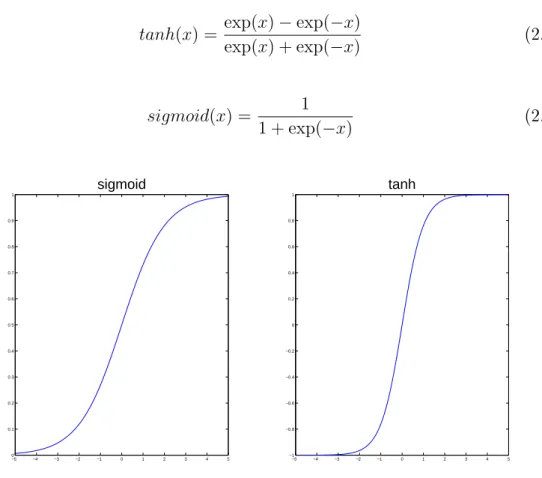
Since the linear discriminant assumes that the classes can be optimally discrimi-nated by a linear discriminant boundary, we cannot use binary threshold activation function in non-linear cases. In nonlinear cases, the output of a perceptron is usually calculated by a nonlinear activation function such as tanh or sigmoid. Note that,
2.3. Articial Neural Networks 11 tanh is a rescaled version of the sigmoid, and its output range is [−1,1] instead of [0,1](Figure 2.2).
tanh(x) = exp(x)−exp(−x)
exp(x) + exp(−x) (2.12) sigmoid(x) = 1 1 + exp(−x) (2.13) −5 −4 −3 −2 −1 0 1 2 3 4 5 0 0.1 0.2 0.3 0.4 0.5 0.6 0.7 0.8 0.9 1 sigmoid −5 −4 −3 −2 −1 0 1 2 3 4 5 −1 −0.8 −0.6 −0.4 −0.2 0 0.2 0.4 0.6 0.8 1 tanh
Figure 2.2 Sigmoid and tanh activation functions
2.3.2 Multilayer perceptron
ANN models are inspired by the human brain and thus mimic human brain. The MLP (also referred to as feedforward networks) is an ANN structure that can be used for regression and classication tasks. MLPs are universal function approximators. The basic processing element of MLP is a perceptron/neuron.
A one-hidden-layer MLP (Figure 2.4) is a functionf :RD → RK, whereDis input
Figure 2.3 Simple perceptron
2.3. Articial Neural Networks 13 f(x) =ϕ(b(2)+V(ϕ(b(1)+W x) | {z } =z(x) )) | {z } =y(x) (2.14)
with bias vectors b(1), b(2); weight matrices W, V and activation function ϕ. The
vectorz(x) = ϕ(b(1)+W x)constitutes the hidden layer which can be considered as a feature extractor. W ∈ RD×Dh is the weight matrix between the input layer and
hidden layer. As activation function ϕ, one can use tanh, sigmoid and/or relu.
The vector y(x) = ϕ(b(2) +V z(x)), where V ∈ RDh×K denotes the weight matrix
between the hidden layer and output layer, constitutes the output layer.
The parameters of MLP to be learnt during training is the set θ =W, V, b(1), b(2) .
The parameters are learnt using (stochastic) gradient descent. The gradients of the error function, ∂E
∂θ, are computed through the backpropagation (BP) algorithm,
which is essentially the chain-rule of derivation.
2.3.3 Autoencoder (Autoassociator)
In Chapter 2.3.2, a common ANN architecture, namely MLP, for supervised learning is discussed. However, we do not have labels all the time since collecting labels is a non-trivial task. In this case, we aim at nding some underlying structure. This branch of machine learning is named as unsupervised learning. If we do not have labels, i.e. if we have only the set of
x(1), x(2), . . . , we can still use an ANN by setting the target values to be equal to the inputs, i.e. y(i) = x(i). This special ANN architecture is a so called autoencoder (autoassociator) and it still uses BP as training algorithm.
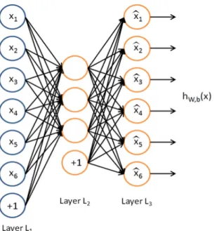
Autoencoder tries to learn a function f = hW,b(x) ≈ x. At rst glance, it might
look like as if autoencoder is trying to learn the identity function which is denitely a trivial function. However, if we impose additional constraints on the network structure (Figure 2.5), for example, restricting the number of hidden neurons, we can discover a useful structure of the data [2]. If there is a structure in the data and if we use fewer neurons in the hidden layer compared to input layer, we can learn a compressed representation. This is similar to principal component analysis (PCA) if we do not use nonlinear activation function in the hidden layer. We can still
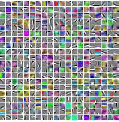
discover interesting structure although we use many hidden neurons by imposing sparsity constraint on the hidden neurons. This type of autoencoder is called as sparse autoencoder. Figure 2.6 shows the learned features on a set of100,000 small 8×8 patches sampled from the larger 96×96 STL-10 1 [3] images using a linear decoder (a sparse autoencoder whose output layer uses a linear activation function). Sparse autoencoder learns features looking like edges and opponent colours as shown in Figure 2.6.
Figure 2.5 Autoencoder example (Layer L2 acts as an encoder and layer L3 acts as a
decoder)
There are dierent variants of autoencoders such as denoising autoencoder [27]. Autoencoder, denoising autoencoder or sparse autoencoder can be stacked to form a deep network. These deep autoencoders can be used to initialize the weights of deep CNNs.
2.3.4 Training ANN
There are two main training procedures for ANNs, namely online learning and batch learning. In online learning, we write the error function on individual instances
1The STL-10dataset contains5000training and8000test examples, with each example being a 96×96labelled colour image belonging to one of ten classes: airplane, bird, car, cat, deer, dog, horse, monkey, ship, truck.
2.3. Articial Neural Networks 15
Figure 2.6 Learned colour features on STL-10 dataset with a sparse autoencoder
whereas in batch learning we write the error function on the entire training dataset X. In the former one, network adapts itself slowly in time since the network param-eters are updated after each instance. In the latter one, we accumulate the changes over entire training set and update the network parameters after a complete pass over the entire training set. Online learning converges faster because there may be similar patterns in the training set, and the stochasticity has an eect like adding noise and may help escape local minima [6]. Online learning is useful for a number of few reasons [6]:
1. It saves the cost of storing the training samples in an external memory and storing the intermediate results during optimization.
2. The problem may be changing in time, which means that the sample distribu-tion is not xed, and a training set cannot be chosen a priori.
A widely used training method for perceptron is stochastic gradient descent and for MLP there is a BP method.
Stochashastic Gradient Descent
For example, if we consider regression problem, the error on the single training instance with index t, (xt, rt), is:
Et(w|xt, rt) = 1 2(r
t−yt)2 = 1
2(r
t−(wTxt))2 (2.15) and for j = 0, . . . , D, the online stochastic update is
∆wtj =−η∂E
t
∂wj
(2.16) =η(rt−yt)xtj (2.17)
where η is the learning parameter. Equation 2.17 can be stated as follows:
U pdate =LearningRate×(DesiredOutput−P redictedOutput)×Input (2.18)
After we compute the update, we update the weights:
wtj =wtj+ ∆wjt (2.19)
For classication problems, the update rules can be derived in a similar way using sigmoid outputs (for 2-class classication problem) or softmax outputs (for K > 2 classes). For example, the output for a single training instance with index t will
be yt =sigmoid(wTxt)for 2-class case. As error function, instead of using squared error, cross-entropy error is more suitable for classication problems. The update rule for cross-entropy error is the same as Equation 2.17.
2.3. Articial Neural Networks 17 Backpropogation
Considering the MLP in Figure 2.4, we assume xj, j = 1, . . . , D are the inputs,
zh, h= 1, . . . , Dh are the hidden units,yi, i= 1, . . . , K are the output units,whj are
the weights between the input layer and hidden layer andvihare the weights between
hidden layer and output layer. Further, we assume sigmoid activation function for the hidden layer and linear activation function for the output layer. Since the hidden layer acts as an input layer to the output layer, we can think of it as a perceptron without loss of generality. Therefore, we already know how to update the parameters
vih given the input zh. In order to update the rst-layer weights, whj, we use the
chain rule to calculate the gradient:
∂E ∂whj = ∂E ∂yi ∂yi ∂zh ∂zh ∂whj (2.20) We can interpret the Equation 2.20 as the error E propagates from the output y
back to the input x through zh. Now, we consider a nonlinear regression problem
to derive the Equation 2.20. In the forward pass, we rst calculate thezh and then
yi. zh =sigmoid(wThx) = 1 1 + exp h −PD j=1whjxj+wh0 i (2.21) yi =vTi z = Dh X h=1 vihzh+vi0 (2.22)
In the backward pass, we start with writing the error function over the entire training set:
E(W, V|X) = 1 2 N X t=1 K X i=1 (rit−yti)2 (2.23)
Next, we write the (batch) update rule for the weights between hidden and output layer: ∆vih =η N X t=1 (rit−yti)zth (2.24)
Note that the only dierence between Equation 2.24 and Equation 2.17 is that the former is written over the entire training set whereas the latter one is written over a single training instance. This is the dierence between the basic and stochastic gradient search.
We cannot use the same update rule as Equation 2.24 to update the weights between input and hidden layer, whj, since we do not have the desired output values for the
hidden layer. We need to apply chain rule: ∆whj =−η ∂E ∂whj (2.25) =−η N X t=1 K X i=1 ∂Et ∂yt i ∂yt i ∂zt h ∂zt h ∂whj (2.26) =−η N X t=1 K X i=1 −(rit−yti) | {z } ∂Et/∂yt i vih |{z} ∂yt i/∂z t h zht(1−zht)xtj | {z } ∂zt h/∂whj (2.27) =η N X t=1 " K X i=1 (rit−yit)vih # zth(1−zht)xtj (2.28)
Gradient descent based training is simple but it converges slowly. In order to im-prove the convergence performance of gradient descent, two methods have been developed, namely momentum and adaptive learning rate. Successive parameter updates of ∆wtj (Equation 2.17), ∆vih (Equation 2.24), ∆whj (Equation 2.25)
2.3. Articial Neural Networks 19 parameter named as momentum, which smooths the gradient using moving average, is introduced. Momentum has an eect of smoothing the trajectory during conver-gence. For example, if we rewrite the Equation 2.17 by taking momentum into account:
∆wjt =−η∂E
t
∂wj
+α∆wt−j 1 (2.29)
where α is generally chosen between 0.5 and 1. Equation 2.29 incorporates the previous update in the current update.
2.3.5 Regularization
In machine learning, most of the time, the trained model performs well on training set. Namely, the resubstitution error (training error) might be severely too opti-mistic. However, for most purposes, we are interested in the performance of unseen test set. In other words, we desire our trained model to perform well enough on test data. This phenomenon is called generalization. The main reason for lack of generalization is using a complex (exible) model. Using a exible model leads to overtting which causes poor generalization. For example, using a 5th order model in polynomial regression for a training set which is sampled from2nd order polyno-mial is an overtting example. The widely used approach to combat overtting is regularization. The basic idea in regularization is to impose prior information about the solution through some nonnegative function. Therefore, we write an augmented error function [6]:
E0(θ|X) = E(θ|X) + ψ P(θ) (2.30) where E is the error on data, P(θ) is the model complexity function and ψ is the
regularization parameter that controls the trade-o between the error in data and model complexity. It penalizes for too exible models. ψ is usually ne-tuned with
cross-validation (Algorithm 1). Regularization is analogous to assumptions made in statistics based methods discussed in Section 2.2.2 in the sense that they try to overcome the ill-posedness problem.
Algorithm 1 Setting regularization parameter ψ using cross-validation
Choose a set of regularization parameters ψ1, . . . , ψA
Choose a set of training and validation set splits{Xi,Vi}Ki=1
for a= 1 to A do for i= 1 toK do θi a= arg minθ[E(θ|Xi) +ψaP(θ)] end for L(ψa) = K1 PK i=1E(θ i a|Vi) end for ψ∗ = arg minψaL(ψa)
here only early stopping andL1/L2 regularization. Early-stopping
As we train ANNs further and further, the training error continues to decrease but at some point the validation error starts to increase. This is the instant when the overtting starts. Training should be stopped early to overcome this problem. Initially, all the parameters, weights in ANN context, are randomly initialized close to 0. As training continues, the most important weights start to move away from 0 and if training continues further on to get less error on the training set, almost all weights are updated away from 0 and become eective parameters [6]. We can think of it as increasing the model complexity P(θ) by adding new parameters to the model.
L1/L2 regularization
In L1/L2 regularization, P(θ) = kθkpp penalizes certain parameter congurations. If we rewrite the error function in Equation 2.23 by changing the parameters {W, V} to θ: E(θ|X) = 1 2 N X t=1 K X i=1 (rti−yti)2 (2.31)
2.4. Deep Convolutional Neural Network 21 then the regularized error function will be:
E0 =E(θ|X) +ψkθkpp (2.32) where kθkp =P|θ|
j=0|θj|p
1p
which is the Lp norm ofθ.
The most commonly used values for p are 1 and 2, hence it is named as L1/L2 regularization. If p= 2, it is also named as weight decay. It penalizes networks with many nonzero weights.
2.4 Deep Convolutional Neural Network
DL is the fastest growing area of machine learning. Note that, DL is used inter-changeably with representation learning or feature learning. DL learns many levels of abstraction, i.e. builds a hierarchical representation (Figure 2.7). If we consider image data, the rst hidden layer represent learn edges of various orientations, the second hidden layer may represent corner, lines, etc. and so on. Although the DL is widely used in many applications such as speech recognition and natural language processing, the breakthrough results have been achieved in object recognition. The researchers from Toronto decreased the error rate from 26.1% to 15.3% in the Im-ageNet2 object recognition competition in 2012 by using a deep CNN [18]. DL
approaches are robust to natural variation in the data. The same network can be used for many dierent applications (generalizable). Namely, a pre-trained network can be used as a feature extractor for a completely dierent problem. This is known as transfer learning. Furthermore, DL methods are massively parallelizable and that is why the computations can be done on Graphical Processing Units (GPUs). CNNs are widely used models for vision tasks. They are also used for 1D signals such as audio data and time series data. There are several parameters in CNN model: width and height of the input (sub)image, kernel (lter) size at each layer, pooling size and CNN structure, i.e. number of layers and neurons at each layer. Moreover, CNN parameters should be set such that the output of nal CNN layer produces scalar, 1×1 feature maps.
CNN training is based on BP algorithm which is discussed in Section 2.3.4 in detail.
Figure 2.7 Learned hierarchical features from a DL algorithm [20]
Training a CNN with BP algorithm requires a lot of training data, which lacks in most of the cases, to have a good generalization performance. A very common trick to solve this problem is to conduct an unsupervised pre-training stage, performed in a greedy layer-wise manner, prior to actual CNN training. In this way, the network weights are initialized with pre-training results instead of being initialized randomly. For example, stacked sparse autoencoder can be used in pre-training phase.
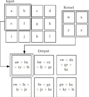
CNNs have two important operators, namely convolution and pooling (subsam-pling). Since the natural images are stationary, which means that the statistics of one part of the image are the same as the other part, convolution is a good operator to learn the same features at all locations. Stationarity is used in the sense that the probability of occurrence of a certain feature (e.g. edge) is the same in every region of the image. A 2D feature map is obtained by the convolution of the input image with a kernel (lter) and adding a bias term and then applying a non-linear activation function. The rectied linear unit (ReLU) [22] is the most widely used activation function in training of deep CNNs. In order to extract dierent features, several feature maps are created at every hidden layer. The second important op-erator of CNNs is pooling. Basically, it decimates the obtained feature maps after convolution by aggregating the statistics feature maps (summary statistics).
2.4.1 Convolution
Convolution is a linear mathematical operation which has many applications in engineering and mathematics. Discrete convolution of the input signalxand weight
2.4. Deep Convolutional Neural Network 23 y[n] =x[n]∗w[n] = ∞ X u=−∞ x[u]w[n−u] = ∞ X u=−∞ x[n−u]w[u] (2.33) y[m, n] =x[m, n]∗w[m, n] = ∞ X u=−∞ ∞ X v=−∞ x[u, v]w[m−u, n−v] (2.34) In DL models, a weightwconsists of a set of learnable parameters. In fact, in CNN
implementations, cross-correlation is used rather than convolution. The expression for cross-correlation looks quite similar to that of the convolution sum given by Equation 2.33 and Equation 2.34. The kernelw is not ipped in cross-correlation
calculation: y[n] =x[n]∗w[−n] = ∞ X u=−∞ x[u]w[−(n−u)] = ∞ X u=−∞ x[−(n−u)]w[u] (2.35) In DL context, both operations are referred to as convolution. Figure 2.8 shows an illustration of 2D convolution without kernel ipping.
Convolution impose three important ideas that can improve a machine learning system: sparse connectivity, weight (parameter) sharing and equivariant represen-tations [4]. Traditional ANNs are fully connected which means that every neuron in a particular layer is connected to every neuron in the next layer. On the contrary, CNNs have sparse interactions because of using a smaller kernel w than the input x. This property reduces the number of free parameters to be learnt and thus
mem-ory requirements. As we know from ltering, same w is convolved with the input x. Namely, weight w is shared. Sparse connectivity and weight sharing properties
of convolution are illustrated in Figure 2.9. The replication of weights (kernels) causes the layer to have the equivariance property to translation [4]. In other words, it allows the same features to be detected invariant to their positions in the input. For example, one layer can detect edges in an image regardless of their positions in the image. However, convolution is not equivariant to other transformations such as scale and rotation.
Figure 2.8 An example of2D convolution without kernel ipping (Source: http: // www.
iro. umontreal. ca/ ~bengioy/ dlbook/ version-07-08-2015/ convnets. html )
Figure 2.9 Illustration for sparse connectivity and weight sharing (Source: http: // deeplearning. net/ )
2.4.2 Pooling (Subsampling)
Using convolved feature maps is impractical due to computational complexity, stor-age requirement and overtting. In order to solve this problem, we need to reduce the dimensionality through a subsampling (downsampling) procedure, namely pool-ing operator. The most popular poolpool-ing functions are max poolpool-ing and mean poolpool-ing. Max-pooling divides the feature map into non-overlapping patches and outputs the maximum value from each patch while mean-pooling outputs the mean value from each patch. To illustrate, we have apply max pooling and mean pooling operators
2.4. Deep Convolutional Neural Network 25 to a subimage I: I = 1 2 3 4 5 6 7 8 9 10 11 12 13 14 15 16 →Imax= " 6 8 14 16 # , Imean= " 3.5 5.5 11.5 13.5 # (2.36)
Pooling is also useful for its ability to make the representation become invariant to translations and rotations of the input.
2.4.3 Rectied Linear Unit (ReLU)
Rectied Linear Unit is a non-saturating activation function in the form of
ϕ(x) = max(0, x) (2.37)
The main advantage of training of deep CNNs with ReLUs over traditional sigmoid or tangent hyperbolic functions is its training speed with gradient descent. Both the ReLUs themselves and their derivatives are computed faster than the other activation functions since it is an if-else check. Although ReLU function is not dierentiable at x= 0, in practice it does not pose a severe problem.
3. METHODOLOGY
In this chapter, the details of the implementation steps for the thesis work are described. These steps mainly consist of preprocessing and CNN structure.
3.1 Preprocessing
Preprocessing plays a crucial role in many machine learning algorithms including DL. With the help of preprocessing, the data is made more robust for learning tasks.
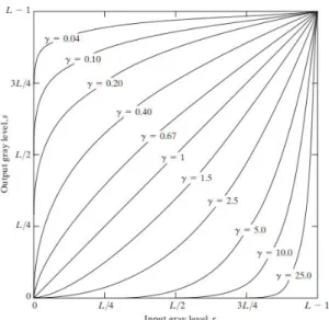
3.1.1 Gamma correction
The original images of SFU subset are nonlinear (γ 6= 1) and thus gamma correction (γ = 2.2) is applied to get almost linear images [14]. Gamma correction is also known as power law transformation which has the basic form [16]:
s=crγ (3.1)
where cand γ are positive constants. In Figure 3.1, r is mapped to s. γ <1 maps a narrow range of dark input values into a wider range of output values whereas
γ >1works in the opposite way.
3.1.2 Image resizing and cropping
Images in Shi-Gehler dataset are resized such that maximum of width and height is 1200, i.e. max(width, height) = 1200. Further, the Macbeth Colour Checker
3.1. Preprocessing 27
Figure 3.1 Plots of Equation 3.1 for various values ofγ (c= 1 in all cases)
(MCC) is removed from every image for training and testing. Images of SFU subset are not resized but the images are cropped to remove the gray ball for the same reason as Shi-Gehler dataset. The resulting images are 240×240 pixels.
3.1.3 Non-overlapping patch extraction
The number of all possible 32×32 patches are quite large in Shi-Gehler dataset. There are more than 500 possible patches per image. Unlike [8], which extracts random patches from the image, only the most 100 brightest patches are extracted from the images in this work. The brightness is dened as the sum of all pixel intensity values of RGB channels in the patch. The brightest pixels has been proved to be useful in illumination estimation process on statistics based algorithms [23]. On the other hand, for SFU subset, there are 100 24×24non-overlapping patches per image after the gray ball is cropped from the images. Since the number of all possible patches are small, we extract and use all 100 patches for SFU subset dataset.
3.1.4 Global histogram stretching
Global histogram stretching is an image enhancement technique which aims to in-crease the dynamic range of the image. It improves an image by stretching the range
of values via a linear mapping T. The rst step is to dene the lower and upper
limits,aandbrespectively, of the output image. For example, for8-bit image,a= 0 and b = 255. In the second step, we nd out the lower and upper limits, c and d
respectively, of the input image. Then, the global histogram stretching mapping
s=T(r) is dened as: s= (r−c) b−a d−c +a (3.2) where r is mapped to s.
After patches are extracted from the colour images, a contrast normalization through global histogram stretching is applied to every patch.
3.1.5 Feature standardization
Zero-mean and unit-variance feature standardization is the most common method for normalization and is widely used, e.g. in ANN and SVM training. In the rst step, the mean of each dimension (across the entire dataset) is computed and then subtracted from each corresponding dimension. In the second step, each dimension is divided by its standard deviation.
x0 = x−x¯
σ (3.3)
where xis the original feature vector, x¯is the mean of that feature vector, and σ is
its standard deviation.
After the contrast normalization is performed, the zero-mean and unit-variance stan-dardization is applied to the patches.
3.2 CNN architecture
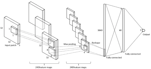
In this thesis, a CNN is used to estimate the colour of the light source from the non-overlapping patches extracted from the raw input colour images. The authors
3.2. CNN architecture 29 of [8] tried dierent parameters including network architecture and concluded that the network architecture shown in Figure 3.2 is the best one for Shi-Gehler dataset. We build our CNN model based on the architecture of [8] for Shi-Gehler dataset as it was proved to be the best network architecture. The network consists of5 layers: 32×32×3 -32×32×240 -4×4×240 -40-3. The rst layer is input layer which takes32×32×3non-overlapping patches. The second layer is a convolutional layer that lters the input patches with 240 dierent kernels, whose size is 1×1×3 with a stride of 1 pixel. The convolutional layer produces 240 dierent feature maps of size 32×32. The third layer is a max-pooling layer with 8×8 kernels and stride of 8 pixels. The results of max-pooling layer are 240 feature maps of size 4×4. The third layer is reshaped from4×4×240into a4×4×240 = 3840vector and is passed through Rectied Linear Units (ReLUs). The fourth layer is a fully connected (FC) layer which consists of 40 neurons. Finally, the fth layer is the output layer which consists 3 neurons for each chromaticity value of r, g and b. However, there is a
minor dierence in the network structure for SFU subset dataset since the input patches are 24×24 instead of 32×32. The network structure is 24×24× 3 -24×24×240 - 3×3×240 - 40- 3.
3.3 CNN training and testing
CNNs are trained with 32×32 and 24×24 image patches for Shi-Gehler and SFU subset datasets, respectively. In the output layer, euclidean loss is used. For Shi-Gehler dataset, error estimates are calculated using 3-fold cross validation. In each run, the CNN is trained with two folds and tested with one fold and this procedure is repeated three times. For SFU subset dataset, error estimates are calculated using 15-fold cross validation. In each run, the CNN is trained with 14 folds and tested with one fold and this procedure is repeated 15 times. In other words, a single experiment is completed after each fold has been used as testing set. The ground truth illuminant of each image is assigned to all patches extracted from that particular image. In testing stage, patches extracted from a particular image are fed to the CNN and CNN outputs predicted patch illuminants. We generate a single global predicted illuminant per image by aggregating patch illuminants. Here, we adopt two dierent pooling strategies, namely mean pooling and median pooling. Mean pooling takes simple average of all predicted patch illuminants in r, g and b
dimensions separately. Median pooling takes the median value of all predicted patch illuminants in r, g and b dimensions separately and can be considered more robust
than mean pooling.
In ANNs, the weights are randomly initialized. Random initialization is a factor determining the performance and the speed of the network. Because of this, we trained the CNN ten times and calculated the error estimates using an average of ten dierent runs. Further, we initialized the kernels using the Xavier algorithm proposed by Bengio's team [15]. The algorithm automatically determines the scale of initialization based on the number of input and output neurons. In training, we choose the parameters given in Table 3.1.
Table 3.1 Parameters in CNN training
Parameter Value
Batch size 100
EPOCH 8
Learning rate 0.1 Weight decay parameter 0.0005
31
4. EXPERIMENTAL SETUP AND RESULTS
In this chapter, experimental setup and results are discussed in detail. The angular error results are presented in tables. Moreover, some example images are shown for visual assessment. The implementation platform for this thesis work was MATLAB. MatConvNet [26], which is a MATLAB toolbox implementing CNNs, is used in the implementation.
4.1 Datasets
The performance of CC algorithms are tested on two standard benchmark (pub-licly available) datasets, re-processed version of Shi-Gehler (Colour Checker) RAW dataset [24] and SFU subset (Grayball subset) [7]. The size of the datasets are small for CNNs, however, since we use image patches as input, we have much larger training datasets.
The Shi-Gehler RAW dataset contains 568indoor and outdoor images (246of them are indoor and 322 of them are outdoor) taken using Canon 5D and Canon 1D digital cameras. The dataset was originally provided by Gehler et. al. [13] and Shi et. al. [24] reprocessed the dataset. The dataset contains linear (gamma=1) almost raw 12-bit PNG format images. The spatial resolution of images which are taken using Canon 1D are 2041× 1359 whereas the spatial resolution of images which are taken using Canon 5D are 2193 ×1460. Canon 1D has a black level of zero while Canon 5D has a black level of 129 which we have to subtract. The three folds are provided with the dataset. The ground truth illuminant of each acquired scene is obtained through the Macbeth ColourChecker (MCC) which is present in every scene. Example images of Shi-Gehler RAW dataset are shown in Figure 4.1. The SFU subset contains 1135 images which are selected from the original SFU dataset [11] (11346real-world images) based on a video-based analysis to reduce the eect of correlation. The images are 8-bit and the spatial resolution of the images
Figure 4.1 Example images of Shi-Gehler RAW dataset
are 240×360 pixels. The SFU images are divided into 15 subcategories based on geographical location and therefore 15-fold cross validation is used. The ground truth illuminant of each scene is obtained through a gray ball which is present in the right-bottom of each image. Example images of SFU subset dataset are shown in Figure 4.2.
Figure 4.2 Example images of SFU subset dataset
4.2 Error Measure
In this thesis, angular error is used as the error metric since it is intuitive and the most widely used error metric in the literature. The error metric which was suggested
4.3. Results 33 in [17] is the angle between the RGB triplet of the ground truth illuminant e and
the RGB triplet of the estimated illuminant eˆ:
angular error= arccos
eTˆe
kek kˆek
(4.1) where k.kis the L2 norm operator.
In Table 4.1 and Table 4.2, the minimum,10th-percentile, median, average (mean), 90th-percentile, and maximum of the angular errors obtained are reported.
4.3 Results
In Table 4.1, the angular error statistics obtained from the statistics based ap-proaches and CNN approach on Shi-Gehler dataset are presented. The reported angular error statistics are the minimum, 10th percentile, median, average, 90the percentile and maximum. The upper block in the table consists the statistics-based algorithms results whereas the bottom block consists CNN results. As can be seen from the table, CNN average-pooling and median-pooling signicantly outperforms statistics based approaches in terms of average, 90th percentile and maximum error. It is possible to see that the improvement is 26.6%, 33.6% and 5.8% respectively. However, in terms of median error, gamut mapping is slightly better than CNN based approach. CNN median-pooling has an angular error 3.9% worse than gamut mapping. However, it is important to note that CNN based results are obtained with same algorithm whereas the best results from statistics based approaches are obtained with dierent algorithms. Figure 4.3 and 4.5 present some corrected images on which CNN approach makes the smallest angular error. On the other hand, Figure 4.4 and 4.6 present some corrected images on which CNN approach makes the largest angular error.
In Table 4.2, the angular error statistics obtained from the statistics based ap-proaches and CNN approach on SFU Subset dataset are presented. Similar to Table 4.1, the reported angular error statistics are the minimum, 10th percentile, median, average,90the percentile and maximum. The upper block in the table con-sists the statistics-based algorithms results whereas the bottom block concon-sists CNN results. As can be seen from the table, CNN average-pooling and median-pooling signicantly outperforms statistics based approaches in terms of average, median
and 90th percentile error. It is possible to see that the improvement is 20%,17.63% and 12.13% respectively. In terms of maximum error, white patch is better than CNN based approach. CNN average-pooling has an angular error 13.9% worse than white patch. Figure 4.7 and 4.9 present some corrected images on which CNN ap-proach makes the smallest angular error. On the other hand, Figure 4.8 and 4.10 present some corrected images on which CNN approach makes the largest angular error.
Algorithm Min 10thprc Med Avg 90thprc Max
Do-Nothing 3.72 10.38 13.55 13.62 16.45 27.37 Gray-World 0.18 1.88 6.30 6.27 10.12 24.84 White-Patch 0.08 1.38 5.61 7.46 15.68 40.59 Shades-of-Gray 0.18 1.04 4.04 4.85 9.71 19.93 general GW 0.03 0.82 3.45 4.60 9.68 22.21 Gray-edge1 0.16 1.82 4.55 5.21 9.78 19.69 Gray-edge2 0.26 2.06 4.43 5.01 8.93 16.87 Gamut-Mapping 0.05 0.40 2.28 4.10 11.08 23.18 CNN per patch 0.00 0.95 2.60 3.46 6.87 29.70 CNN avg.-pooling 0.09 0.90 2.42 3.05 6.19 15.89 CNN med.-pooling 0.08 0.90 2.37 3.01 5.93 17.39
Table 4.1 Angular error statistics on linear Shi-Gehler RAW dataset
Algorithm Min 10thprc Med Avg 90thprc Max
Do-Nothing 0.48 1.55 14.55 15.69 33.91 41.57 Gray-World 0.09 2.91 10.75 12.97 26.09 56.39 White-Patch 0.33 1.95 10.33 12.73 26.62 39.59 Shades-of-Gray 0.05 3.08 9.77 11.60 22.16 49.95 Gray-edge1 0.10 2.78 9.14 11.13 21.19 54.04 Gray-edge2 0.15 2.87 9.43 10.89 21.18 45.77 Gamut-Mapping 0.29 2.60 11.98 14.18 29.65 43.86 CNN per patch 0.01 2.26 8.21 10.43 21.88 61.53 CNN avg.-pooling 0.15 2.09 7.53 9.18 18.81 45.11 CNN med.-pooling 0.15 2.05 7.23 8.97 18.61 48.84
4.3. Results 35
4.3. Results 37
4.3. Results 39
Figure 4.7 Best mean pooling CNN result in SFU subset
Figure 4.9 Best median pooling CNN result in SFU subset
41
5. CONCLUSIONS
In this thesis, we have studied DL architectures, namely deep CNNs, to learn CC. The motivation was to show that CNNs are very good models not only for recognition tasks but also for low level computer vision problems. Unlike existing learning based methods that rely on hand-crafted, low level visual features, we propose to use CNNs to learn hierarchical feature representations to achieve robust CC.
CNNs, probably the most popular DL models, are biologically inspired variants of MLPs. Both CNNs and MLPs are trained with BP algorithm. However, there are two essential dierences of CNNs compared to MLPs. First, CNNs are not fully connected as MLPs. CNNs exploit local connectivity structure, which is usually referred to as receptive eld, of the data. This property leads to sparse connectivity. Second, the parameters (weights) are shared in CNNs. In fact, sparse connectivity and weight sharing are a constraint of CNN model but this constraint enables CNNs to achieve good performance e.g. on vision tasks when the amount of data is limited. Using CNNs for CC is a quite new idea and, to our knowledge, [8] is the only work that investigates the use of CNNs for illuminant estimation. Unlike [8], which extracts almost all possible patches from the images of Shi-Gehler dataset, only the most 100 brightest patches are extracted from the images in this work. This intelligent patch extraction signicantly reduces the computational burden. As pre-processing, all extracted patches are contrast normalized via global histogram stretching. After contrast normalization, zero mean unit variance feature standard-ization is applied. Instead of traditional sigmoid or tanh non-linear activation func-tions, ReLUs are used in the fully connected layer. During testing phase, illuminant estimation of patches for every test image are aggregated, e.g. mean pooling and median pooling, to generate a single illuminant estimation per image.
Two CNN models are trained to learn the CC and tested on two widely used datasets in MATLAB environment. We evaluated the performance of our CNN models based on cross-validation error rate. The experimental results show that CNN-based CC
outperforms almost all the traditional approaches both in Shi-Gehler dataset and in SFU subset dataset. It is important to note that the best results from statistics based approaches are obtained from dierent algorithms and selection of best algorithm is an on-going research topic. On the other hand, CNN based results are obtained from a single algorithm.
43
BIBLIOGRAPHY
[1] http://colorconstancy.com/, (accessed September 13, 2015).
[2] http://deeplearning.stanford.edu/wiki/index.php/Autoencoders_and_ Sparsity, (accessed September 13, 2015).
[3] http://cs.stanford.edu/~acoates/stl10/, (accessed September 13, 2015).
[4] http://www.iro.umontreal.ca/~bengioy/dlbook/convnets.html, (accessed September 13, 2015).
[5] V. Agarwal, A. V. Gribok, and M. A. Abidi, Machine learning approach to color constancy, Neural Networks, vol. 20, no. 5, pp. 559 563, 2007. [Online]. Available: http://www.sciencedirect.com/science/article/pii/ S0893608007000846
[6] E. Alpaydin, Introduction to Machine Learning, 2nd ed. The MIT Press, 2010. [7] S. Bianco, G. Ciocca, C. Cusano, and R. Schettini, Improving color constancy using indoor-outdoor image classication, Image Processing, IEEE Transac-tions on, vol. 17, no. 12, pp. 23812392, Dec 2008.
[8] S. Bianco, C. Cusano, and R. Schettini, Color constancy using cnns, in Com-puter Vision and Pattern Recognition Workshops (CVPRW), 2015 IEEE Con-ference on, June 2015, pp. 8189.
[9] G. Buchsbaum, A spatial processor model for object colour perception, J. Franklin Inst., vol. 310, pp. 126, 1980.
[10] V. C. Cardei, B. Funt, and K. Barnard, Estimating the scene illumination chromaticity by using a neural network, JOURNAL OF THE OPTICAL SO-CIETY OF AMERICA A, vol. 19, no. 12, pp. 23742386, 2002.
[11] F. Ciurea and B. V. Funt, A large image database for color constancy research. in Color Imaging Conference. IST - The Society for Imaging Science and Technology, 2003, pp. 160164. [Online]. Available: http: //dblp.uni-trier.de/db/conf/imaging/cic2003.html#CiureaF03
[12] B. V. Funt and W. Xiong, Estimating illumination chromaticity via support vector regression, in The Twelfth Color Imaging Conference: Color Science and Engineering Systems, Technologies, Applications, CIC 2004, Scottsdale, Arizona, USA, November 9-12, 2004, 2004, pp. 4752. [Online]. Available: http://www.ingentaconnect.com/content/ist/cic/2004/00002004/ 00000001/art00010
[13] P. Gehler, C. Rother, A. Blake, T. Minka, and T. Sharp, Bayesian color con-stancy revisited, in Computer Vision and Pattern Recognition, 2008. CVPR 2008. IEEE Conference on, June 2008, pp. 18.
[14] A. Gijsenij, T. Gevers, and J. van de Weijer, Computational color constancy: Survey and experiments, Image Processing, IEEE Transactions on, vol. 20, no. 9, pp. 24752489, Sept 2011.
[15] X. Glorot and Y. Bengio, Understanding the diculty of training deep feed-forward neural networks, in In Proceedings of the International Conference on Articial Intelligence and Statistics (AISTATS). Society for Articial Intelli-gence and Statistics, 2010.
[16] R. C. Gonzalez and R. E. Woods, Digital Image Processing (3rd Edition). Up-per Saddle River, NJ, USA: Prentice-Hall, Inc., 2006.
[17] S. Hordley and G. Finlayson, Re-evaluating colour constancy algorithms, in Pattern Recognition, 2004. ICPR 2004. Proceedings of the 17th International Conference on, vol. 1, Aug 2004, pp. 7679 Vol.1.
[18] A. Krizhevsky, I. Sutskever, and G. E. Hinton, Imagenet classication with deep convolutional neural networks, in Advances in Neural Information Pro-cessing Systems, p. 2012.
[19] E. H. Land, John, and J. Mccann, Lightness and retinex theory, Journal of the Optical Society of America, pp. 111, 1971.
[20] H. Lee, R. Grosse, R. Ranganath, and A. Y. Ng, Unsupervised learning of hierarchical representations with convolutional deep belief networks, Commun. ACM, vol. 54, no. 10, pp. 95103, Oct. 2011. [Online]. Available: http://doi.acm.org/10.1145/2001269.2001295
[21] T. M. Mitchell, Machine Learning, 1st ed. New York, NY, USA: McGraw-Hill, Inc., 1997.
Bibliography 45 [22] V. Nair and G. E. Hinton, Rectied linear units improve restricted boltzmann machines. in Proc. 27th International Conference on Machine Learning, 2010. [23] H. Reza, V. Joze, M. S. Drew, G. D. Finlayson, P. Aurora, and T. Rey, The
role of bright pixels in illumination estimation.
[24] L. Shi and B. V. Funt, Re-processed version of the gehler color constancy dataset of 568 images, http://www.cs.sfu.ca/~colour/data/, (accessed Septem-ber 13, 2015).
[25] J. van de Weijer, T. Gevers, and A. Gijsenij, Edge-based color constancy, Image Processing, IEEE Transactions on, vol. 16, no. 9, pp. 22072214, Sept 2007.
[26] A. Vedaldi and K. Lenc, Matconvnet convolutional neural networks for mat-lab, CoRR, vol. abs/1412.4564, 2014.
[27] P. Vincent, H. Larochelle, Y. Bengio, and P.-A. Manzagol, Extracting and composing robust features with denoising autoencoders, in Proceedings of the 25th International Conference on Machine Learning, ser. ICML '08. New York, NY, USA: ACM, 2008, pp. 10961103. [Online]. Available: http://doi.acm.org/10.1145/1390156.1390294

![Figure 2.7 Learned hierarchical features from a DL algorithm [20]](https://thumb-us.123doks.com/thumbv2/123dok_us/361653.2539838/33.892.175.803.114.273/figure-learned-hierarchical-features-dl-algorithm.webp)