July 2010, Volume 35, Issue 9. http://www.jstatsoft.org/
JM: An
R
Package for the Joint Modelling of
Longitudinal and Time-to-Event Data
Dimitris RizopoulosErasmus University Medical Center
Abstract
In longitudinal studies measurements are often collected on different types of outcomes for each subject. These may include several longitudinally measured responses (such as blood values relevant to the medical condition under study) and the time at which an event of particular interest occurs (e.g., death, development of a disease or dropout from the study). These outcomes are often separately analyzed; however, in many instances, a joint modeling approach is either required or may produce a better insight into the mechanisms that underlie the phenomenon under study. In this paper we present the
RpackageJMthat fits joint models for longitudinal and time-to-event data.
Keywords: attrition, dropout, longitudinal data, shared parameter models, survival data, time-dependent covariates.
1. Introduction
Longitudinal studies often produce two types of outcome, namely a set of longitudinal response measurements and the time to an event of interest, such as death, development of a disease or dropout from the study. Two typical examples of this setting are HIV and cancer studies. In HIV studies patients who have been infected are monitored until they develop AIDS or die, and they are regularly measured for the condition of the immune system using markers such as the CD4 lymphocyte count or the estimated viral load. Similarly in cancer studies the event outcome is the death or metastasis and patients also provide longitudinal measurements of antibody levels or of other markers of carcinogenesis, such as the PSA levels for prostate cancer.
These two outcomes are often separately analyzed using a mixed effects model for the longitu-dinal outcome and a survival model for the event outcome. However, in mainly two settings a joint modelling approach is required. First, when interest is on the event outcome and we wish to account for the effect of the longitudinal outcome as a time-dependent covariate, traditional approaches for analyzing time-to-event data (such as the partial likelihood for the Cox proportional hazards models) are not applicable. In particular, standard time-to-event models require that time-dependent covariates are external; that is, the value of this covari-ate at time pointt is not affected by the occurrence of an event at time point u, with t > u (Kalbfleisch and Prentice 2002, Section 6.3). However, the type of time-dependent covariates encountered in longitudinal studies do not satisfy this condition, due to the fact that they are the output of a stochastic process generated by the subject, which is directly related to the failure mechanism. Therefore, in order to produce valid inferences a model for the joint distribution of the longitudinal and survival outcomes is required instead. The second setting in which joint modelling is required is when interest is on the longitudinal outcome. In this case the occurrence of events causes dropout since no longitudinal measurements are available at and after the event time. When this dropout is nonrandom (i.e., when the probability of dropout depends on unobserved longitudinal responses), then bias may arise from an analysis that ignores the dropout process (Little and Rubin 2002, Chapter 15). To avoid this problem and obtain valid inferences the longitudinal and dropout process must be jointly modelled. One of the modelling frameworks that have been proposed in the missing data literature for
handling nonrandom dropout is the shared parameter model (Follmann and Wu 1995), which
postulates a mixed effects model for the longitudinal outcome and time-to-dropout model for the missingness process. In both settings the joint distribution of the event times and the longitudinal measurements is modelled via a set of random effects that are assumed to account for the associations between these two outcomes. Excellent overviews of this area of biostatistics and statistics research are given by Tsiatis and Davidian (2004) and Yu, Law, Taylor, and Sandler(2004).
Software for the separate analysis of longitudinal and event time data has been available for
many years. For instance, in R (R Development Core Team 2010) several packages provide
functions for fitting mixed effects models, such as package nlme (Pinheiro, Bates, DebRoy, Sarkar, and RDevelopment Core Team 2009) and package lme4 (Bates and Maechler 2010),
and for survival models package survival (Therneau and Lumley 2009) – for a more
com-prehensive list of the available packages in the Comcom-prehensive R Archive Network (CRAN)
relevant to the analysis of event time data we refer to the CRAN task view “Survival Anal-ysis” (Allignol and Latouche 2010). In this paper we focus in the joint modelling of
longi-tudinal and time-to-event data, and we present the Rpackage JM (available from CRAN at
http://CRAN.R-project.org/package=JM) that can be used to fit such joint models. The
implementation of joint models inSASandWinBUGShas been discussed byGuo and Carlin
(2004). The rest of the paper is organised as follows. In Section2 we present the joint mod-elling framework, and discuss different choices for the time-to-event submodel. Furthermore, we describe the basics of maximum likelihood estimation for this type of models, with special mention to numerical integration techniques. In addition, we refer to several types of residuals and prediction of conditional probabilities of survival. Section3describes in detail the imple-mentation of the theory described in Section 2 in package JM. Finally, Section 4 illustrates the capabilities of the package in a real data example from HIV research, and Section5gives some concluding remarks.
2. Joint modelling framework
2.1. Submodels specification
In the following we will present the joint modelling framework motivated by the time-to-event point of view (i.e., in the setting in which we want to incorporate a time-dependent covariate measured with error in a survival model) – a more direct connection with the missing data framework is made in Section 2.3. Let Ti denote the observed failure time for thei-th subject (i = 1, . . . , n), which is taken as the minimum of the true event time Ti∗ and the censoring time Ci, i.e., Ti = min(Ti∗, Ci). Furthermore, we define the event indicator as
δi = I(Ti∗ ≤Ci), where I(·) is the indicator function that takes the value 1 if the condition
Ti∗ ≤Ci is satisfied, and 0 otherwise. Thus, the observed data for the time-to-event outcome consist of the pairs{(Ti, δi), i= 1, . . . , n}. For the longitudinal responses, letyi(t) denote the value of the longitudinal outcome at time pointt for the i-th subject. We should note here that we do not actually observeyi(t) at all time points, but only at the very specific occasions
tij at which measurements were taken. Thus, the observed longitudinal data consist of the
measurements yij ={yi(tij), j = 1, . . . , ni}.
Our aim is to associate the true andunobserved value of the longitudinal outcome at time t, denoted by mi(t), with the event outcome Ti∗. Note that mi(t) is different from yi(t), with the latter being the contaminated with measurement error value of the longitudinal outcome at timet. To quantify the effect ofmi(t) on the risk for an event, a standard option is to use a relative risk model of the form (Therneau and Grambsch 2000):
hi(t| Mi(t), wi) = lim dt→0Pr{t≤T ∗ i < t+dt|T ∗ i ≥t,Mi(t), wi}/dt = h0(t) exp{γ>wi+αmi(t)}, (1)
where Mi(t) = {mi(u),0 ≤ u < t} denotes the history of the true unobserved longitudinal process up to time pointt,h0(·) denotes the baseline risk function, andwiis a vector of baseline covariates (such as a treatment indicator, history of diseases, etc.) with a corresponding vector of regression coefficients γ. Similarly, parameter α quantifies the effect of the underlying longitudinal outcome to the risk for an event; for instance, in the AIDS example mentioned in Section1,αmeasures the effect of the number of CD4 cells to the risk for death. To avoid the impact of parametric assumptions, the baseline risk functionh0(·) is typically left unspecified.
However, within the joint modelling frameworkHsieh, Tseng, and Wang(2006) have recently noted that leaving this function completely unspecified leads to an underestimation of the standard errors of the parameter estimates. In particular, problems arise due to the fact that the nonparametric maximum likelihood estimate for this function cannot be obtained explicitly under the full joint modelling approach. To avoid this problem, we could either opt for the hazard function of a standard survival distribution (such as the Weibull or Gamma) or for more flexible models in whichh0(t) is sufficiently approximated using step functions or
spline-based approaches.
An alternative modelling framework for event time data, especially when the proportionality assumption in (1) fails, is the accelerated failure time model. In order to incorporate a time-dependent covariate within this framework, we letS0denote an absolutely continuous baseline
postulates
nZ T
∗
0
exp{γ>w+αm(s)}dso∼ S0.
This can be reexpressed in terms of the risk rate function for subjectias:
hi(t| Mi(t), wi) = h0{Vi(t)}exp{γ>wi+αmi(t)}, (2) with Vi(t) = Z t 0 exp{γ>wi+αmi(s)}ds.
Similarly, to (1), the baseline risk functionh0(·) can be assumed of a specific parametric form
or modelled flexibly. An important difference of (2) compared to (1) is that in the former the entire covariate historyMi(t) is assumed to influence the subject-specific risk (due to the fact that h0(·) is evaluated at Vi(t)), whereas in the latter the subject-specific risk depends only on the current value of the time-dependent covariate mi(t). The survival function for a subject with covariate history Mi(t) equals Si{t| Mi(t)} =S0{Vi(t)}, which means that this subject ages on an accelerated scheduleVi(t) compared to S0 – for more information we
refer toCox and Oakes(1984, Section 5.2). Within the joint modelling framework accelerated failure time models have been discussed byTseng, Hsieh, and Wang (2005).
In the definitions of the survival models presented above we used mi(t) to denote the true
value of the underlying longitudinal covariate at time point t. However and as mentioned
earlier, longitudinal information is actually collected intermittently and with error at a set of few time pointstij for each subject. Therefore, in order to measure the effect of this covariate to the risk for an event we need to estimate mi(t) and successfully reconstruct the complete longitudinal history Mi(t), using the available measurements yij = {yi(tij), j = 1, . . . , ni} of each subject and a set of modelling assumptions. For the remaining of this paper we will focus on normal data and we will postulate a linear mixed effects model to describe the subject-specific longitudinal evolutions. In particular, we have
yi(t) = mi(t) +εi(t)
= x>i (t)β+zi>(t)bi+εi(t), εi(t)∼ N(0, σ2), (3)
where β denotes the vector of the unknown fixed effects parameters, bi denotes a vector
of random effects, xi(t) and zi(t) denote row vectors of the design matrices for the fixed and random effects, respectively, and εi(t) is the measurement error term, which is assumed independent of bi, and with variance σ2. We should note that care should be taken in the specification of xi(t) and zi(t) in order to produce a good estimate of Mi(t). The main reason for this is that, as we will see later in Section2.2, in the definition of the likelihood of the joint model the complete longitudinal history is required for the computation of the survival function, and of the risk function under the accelerated failure time formulation. Therefore, in applications in which subjects show highly nonlinear longitudinal trajectories, it is advisable to consider flexible representations for xi(t) and zi(t) using a possibly high-dimensional vector of functions of time t, expressed in terms of high-order polynomials or
splines (Ding and Wang 2008; Brown, Ibrahim, and DeGruttola 2005). Finally, in order to
complete the specification of the longitudinal submodel a suitable distributional assumption for the random effects component is required. A standard choice for this distribution is the multivariate normal distribution; however, within the joint modelling framework and mainly
because of the nonrandom dropout (see also Section2.3), there is the concern that relying on a standard parametric distribution may influence the derived inferences especially when this distribution differs considerably from the true random effects distribution. This motivated
Song, Davidian, and Tsiatis(2002) to propose a more flexible model for the distribution of the random effects that is expressed as a normal density times a polynomial function. However, the findings of these authors suggested that the parameter estimates and standard errors of joint models fitted under the normal assumption for the random effects were rather robust to misspecification. This feature has been further theoretically corroborated byRizopoulos, Verbeke, and Molenberghs(2008), who showed that as the number of repeated measurements per subject ni increases, a misspecification of the random effects distribution has a minimal
effect in parameter estimators and standard errors. Thus, here we will assume that bi ∼
N(0, D) and we will not further investigate this assumption.
2.2. Maximum likelihood estimation
The main estimation methods that have been proposed for joint models are (semiparametric)
maximum likelihood (Hsiehet al.2006;Henderson, Diggle, and Dobson 2000;Wulfsohn and
Tsiatis 1997) and Bayes using MCMC techniques (Chi and Ibrahim 2006;Brown and Ibrahim 2003; Wang and Taylor 2001; Xu and Zeger 2001). Moreover, Tsiatis and Davidian (2001) have proposed a conditional score approach in which the random effects are treated as nuisance parameters, and they developed a set of unbiased estimating equations that yields consistent and asymptotically normal estimators. Here we give the basics of the maximum likelihood method for joint models as the one of the more traditional approaches.
Maximum likelihood estimation for joint models is based on the maximization of the log-likelihood corresponding to the joint distribution of the time-to-event and longitudinal out-comes {Ti, δi, yi}. To define this joint distribution we will assume that the vector of time-independent random effects bi underlies both the longitudinal and survival processes. This means that these random effects account for both the association between the longitudinal and event outcomes, and the correlation between the repeated measurements in the longitudinal process (conditional independence). Formally we have that,
p(Ti, δi, yi|bi;θ) = p(Ti, δi|bi;θ)p(yi |bi;θ) (4)
p(yi|bi;θ) =
Y
j
p{yi(tij)|bi;θ}, (5)
where θ = (θ>t , θ>y, θ>b )> denotes the parameter vector, with θt denoting the parameters for the event time outcome, θy the parameters for the longitudinal outcomes and θb the unique parameters of the random-effects covariance matrix, yi is the ni ×1 vector of longitudinal responses of the i-th subject, and p(·) denotes an appropriate probability density function. Due to the fact that the survival and longitudinal submodels share the same random effects, joint models of this type are also known as shared parameter models. Under the modelling as-sumptions presented in the previous section, and these conditional independence asas-sumptions the joint log-likelihood contribution for the i-th subject can be formulated as
logp(Ti, δi, yi;θ) = log Z p(Ti, δi |bi;θt, β) hY j p{yi(tij)|bi;θy} i p(bi;θb)dbi, (6) where the likelihood of the survival part is written as
withhi(·) given by either (1) or (2), and Si(t| Mi(t), wi;θt, β) = Pr(Ti∗ > t| Mi(t), wi;θt, β) = exp − Z t 0 hi(s| Mi(s);θt, β)ds , (8)
p{yi(tij)|bi;θy}is the univariate normal density for the longitudinal responses, and p(bi;θb) is the multivariate normal density for the random effects.
Maximization of the log-likelihood function corresponding to (6) with respect to θ is a com-putationally challenging task. This is mainly because both the integral with respect to the random effects in (6), and the integral in the definition of the survival function (8) do not have an analytical solution, except in very special cases. Standard numerical integration tech-niques such as Gaussian quadrature and Monte Carlo have been successfully applied in the joint modelling framework (Song et al. 2002; Henderson et al. 2000; Wulfsohn and Tsiatis 1997). Furthermore,Rizopoulos, Verbeke, and Lesaffre(2009) have recently discussed the use of Laplace approximations for joint models, that can be especially useful in high-dimensional random effects settings (e.g., when splines are used in the random effects design matrix). For the maximization of the approximated log-likelihood the Expectation-Maximization (EM) algorithm has been traditionally used in which the random effects are treated as ‘missing data’. The main motivation for using this algorithm is the closed-form M-step updates for certain parameters of the joint model. However, a serious drawback of the EM algorithm is its linear convergence rate that results in slow convergence especially near the maximum. Nonetheless, Rizopouloset al. (2009) have noted that a direct maximization of the observed data log-likelihood, using for instance, a quasi-Newton algorithm (Lange 2004), requires very similar computations to the EM algorithm. Therefore hybrid optimization approaches that start with EM and then continue with direct maximization can be easily employed.
2.3. Residuals
A traditional approach to check model assumptions is the inspection of residual plots. Prop-erties and features of residuals, when longitudinal and survival outcomes are separately mod-elled, have been extensively studied in the literature. For instance, different types of residuals
for linear mixed models are discussed in Nobre and Singer (2007) and Verbeke and
Molen-berghs (2000), whereas residuals for parametric and semiparametric survival models are
pre-sented in Harrell (2001) and Therneau and Grambsch (2000). However, calculating these
residuals based on the fitted joint model and the observed data, and then using them to check the model assumptions may prove problematic. In particular, complications arise due to the nonrandom dropout in the longitudinal process caused by the occurrence of events. To show this more clearly, we define for each subject the observed and missing part of the longitudinal response vector. The observed partyoi ={yi(tij) :tij < Ti, j= 1, . . . , ni}contains all observed
longitudinal measurements of the i-th subject before the observed event time, whereas the
missing part ymi = {yi(tij) :tij ≥ Ti, j = 1, . . . , n0i} contains the longitudinal measurements that would have been taken until the end of the study, had the event not occurred. Under these definitions and the assumptions of the joint modelling framework, we can derive the dropout mechanism, which is the conditional distribution of the time-to-dropout given the complete vector of longitudinal responses (yio, ymi ),
p(Ti∗ |yio, ymi ;θ) =
Z
We observe that the time-to-dropout depends onyimthrough the posterior distribution of the random effectsp(bi | yoi, ymi ;θ). This in practice implies that the observed data, upon which the residuals are calculated, are not a random sample of the target population, and therefore should not be expected to exhibit the standard properties of zero mean, constant variance, etc.
To overcome this problem and produce residuals that can be readily used in diagnostic plots for joint models,Rizopoulos, Verbeke, and Molenberghs(2010) have recently proposed to aug-ment the observed data with randomly imputed longitudinal responses under the complete data model, corresponding to the longitudinal outcomes that would have been observed had the patients not dropped out. To present this idea briefly, we assume that the joint model has been fitted to the data set at hand, and that we have obtained the maximum likelihood estimates ˆθ and an estimate of their asymptotic covariance matrix, say ˆH. Moreover, we assume that longitudinal measurements are planned to be taken at prespecified time points t0, t1, . . . , tmax, and that for the i-th subject measurements are available up to the last pre-specified visit time earlier thanTi. In the following we adopt a Bayesian point of view for the
joint modelling framework, since multiple imputation has Bayesian grounds (Little and
Ru-bin 2002, Chapter 10). Multiple imputation is based on repeated sampling from the posterior distribution of ymi given the observed data, averaged over the posterior of the parameters. Under joint model (6) and dropout mechanism (9), the density for this distribution can be expressed as
p(yim|yio, Ti, δi) =
Z
p(ymi |yio, Ti, δi;θ)p(θ|yio, Ti, δi)dθ. (10) The first part of the integrand in (10) can be derived from (9) taking also into account assumptions (4) and (5), i.e.,
p(yim|yio, Ti, δi;θ) = Z p(ymi |bi, yio, Ti, δi;θ)p(bi|yio, Ti, δi;θ)dbi = Z p(ymi |bi;θ)p(bi |yio, Ti, δi;θ)dbi. (11) For the second part, which is the posterior distribution of the parameters given the observed data, we use arguments of standard asymptotic Bayesian theory (Cox and Hinkley 1974, Sec-tion 10.6), and assume that the sample size nis sufficiently large such that{θ|yo
i, Ti, δi}can
be well approximated by N(ˆθ,Hˆ). This assumption, combined with (10) and (11), suggests the following simulation scheme:
1. Drawθ(`)∼ N(ˆθ,Hˆ). 2. Drawb(i`) ∼ {bi |yio, Ti, δi, θ(`)}. 3. Draw yim(`)(tij) ∼ N n µ(il)(tij),σˆy2,(`) o
, for the prespecified visit times tij ≥ Ti, j = 1, . . . , n0i that were not observed for the i-th subject, where µ(il)(tij) = x>i (tij) ˆβ(`)+
zi>(tij)ˆb(i`).
4. Repeat Steps 1–3 for each subject, `= 1, . . . , L times, where L denotes the number of imputations.
Steps 1 and 2 account for uncertainties in the parameters and empirical Bayes estimates, respectively, whereas Step 3 imputes the missing longitudinal responses (more information
can be found inRizopoulos et al.2010). The benefit of using the simulated yim(`)(tij) values together with yoi to calculate residuals is that these residuals inherit now the properties of the complete data model, and therefore they can be directly used in diagnostic plots without requiring to take dropout into account.
2.4. Expected survival
The calculation of predicted survival probabilities based on a fitted survival model on some ref-erence population has received a lot of attention in the statistical literature – see for instance,
Therneau and Grambsch (2000, Chapter 10) and references therein. In this section we focus on expected survival but within the joint modelling framework. In particular, based on a joint model fitted on sample of size n, we are interested in predicting survival probabilities for a new subjectithat has provided a set of longitudinal measurementsYi(t) ={yi(s),0≤s≤t} (dependence on baseline covariates is assumed but is suppressed here for ease of exposition). Note that in the joint modelling framework, providing longitudinal measurements up to time point t in fact implies survival up to time t. Thus, we are actually interested in estimating the conditional probability
πi(u|t) = Pr(Ti∗≥u|T
∗
i > t,Yi(t),Dn), (12) where u > t and Dn denotes the sample on which the joint model was fitted. Similarly to Section 2.3, it is convenient to proceed using a Bayesian formulation of the problem. More specifically, (12) can be written as
Pr(Ti∗≥u|Ti∗ > t,Yi(t),Dn) =
Z
Pr(Ti∗ ≥u|Ti∗> t,Yi(t);θ)p(θ| Dn)dθ. (13) The first part of the integrand and using assumption (4) is given by
Pr(Ti∗ ≥u|Ti∗> t,Yi(t);θ) = Z Pr(Ti∗ ≥u|Ti∗ > t,Yi(t), bi;θ)p(bi |Ti∗> t,Yi(t);θ)dbi = Z Pr(Ti∗ ≥u|Ti∗ > t, bi;θ)p(bi |Ti∗> t,Yi(t);θ)dbi = Z S i{u| Mi(u, bi, θ);θ} Si{t| Mi(t, bi, θ);θ} p(bi|Ti∗ > t,Yi(t);θ)dbi, (14) where Si(·) is given by (8), and furthermore we have explicitly noted that the longitudinal history Mi(·), as estimated by the linear mixed effects model, is a function of both the random effects and the parameters. For the second part we again follow asymptotic Bayesian
arguments and assume that {θ | Dn} can be well approximated by a multivariate normal
distribution with mean the maximum likelihood estimates ˆθ and covariance matrix ˆH =
vˆar(ˆθ). Combining (13) with (14) and {θ | Dn} ∼ N(ˆθ,Hˆ), a Monte Carlo estimate of πi(u|t) can be obtained using the following simulation scheme:
1. Drawθ(`)∼ N(ˆθ,Hˆ).
2. Drawb(i`) ∼ {bi |Ti∗> t,Yi(t), θ(`)}.
4. Repeat Steps 1–3 for each subject, `= 1, . . . , L times, where L denotes the number of Monte Carlo samples.
Step 1 is straightforward to perform; on the contrary, the posterior distribution for the
random effects given the observed data for subject i in Step 2 is of a non-standard form,
and thus a more sophisticated approach is required to sample from it. Here we use of
a Metropolis-Hastings algorithm with independent proposals from a multivariate t
distri-bution centered at the empirical Bayes estimates ˆbi = arg maxb{logp(Ti∗ > t,Yi(t), b; ˆθ)} (where logp(Ti∗ > t,Yi(t), b; ˆθ) = logSi(t | b; ˆθ) + logp(Yi(t) | b; ˆθ) + logp(b; ˆθ)), with scale matrix var(ˆbi) = {−∂2logp(Ti∗ > t,Yi(t), b; ˆθ)/∂b>∂b |b=ˆbi}−1, and four degrees of
freedom. We expect the multivariate t proposals to work satisfactorily in this setting
be-cause, as it has been recently shown by Rizopoulos et al. (2008), as ni (the number of
longitudinal measurements for subject i) increases, the leading term of the log posterior
distribution of the random effects is the logarithm of the density of the linear mixed model logp(Yi(t)|bi;θ(`)) =Pjlogp{yi(tij)|bi;θ(`)}, which is quadratic inbiand will resemble the shape of a multivariate normal distribution. The realizations {π(i`)(u |t), ` = 1, . . . , L} can be used to derive estimates of πi(u|t), such as
ˆ πi(u|t) = median{π (`) i (u|t), `= 1, . . . , L} or ˆπi(u|t) =L−1 L X `=1 π(i`)(u|t), and confidence intervals using the Monte Carlo sample percentiles.
3. The
R
package
JM
3.1. Design
The RpackageJMhas been developed to fit a variety of joint models for normal longitudinal
responses and time-to-event data under maximum likelihood. This package has a single
model-fitting function called jointModel(), which accepts as main arguments a linear mixed effects object fit as returned by function lme() of package nlme, and a survival object fit as
returned by either function coxph()or function survreg()of package survival. The method
argument of jointModel() specifies the type of the survival submodel to be fitted and the
type of numerical integration method; available options are:
method = "weibull-AFT-GH": the Weibull model under the accelerated failure time
for-mulation (i.e., model (2) with h0(·) being the Weibull baseline risk function). The
Gauss-Hermite integration rule is used to approximate integral (6).
method = "weibull-PH-GH": the Weibull model under the relative risk formulation (i.e.,
model (1) with h0(·) being the Weibull baseline risk function). The Gauss-Hermite
integration rule is used to approximate integral (6).
method = "piecewise-PH-GH": the relative risk model (1) with a piecewise-constant
base-line risk function. In particular, h0(t) =
Q
X
q=1
where 0 = v0 < v1 < · · · < vQ denotes a split of the time scale, with vQ being larger than the largest observed time, and ξq denotes the value of the hazard in the interval (vq−1, vq]. The Gauss-Hermite integration rule is used to approximate integral (6).
method = "Cox-PH-GH": the relative risk model (1) with an unspecified baseline risk
func-tion. The Gauss-Hermite integration rule is used to approximate integral (6). This
option corresponds to the joint model proposed by Wulfsohn and Tsiatis (1997).
method = "spline-PH-GH": the relative risk model (1) with a spline-approximated baseline
risk function. In particular, the log baseline risk function logh0(t) is expanded into
B-spline basis functions as follows,
logh0(t) =κ0+
m
X
d=1
κdBd(t, q),
where κ> = (κ0, κ1, . . . , κm) are the spline coefficients, q denotes the degree of the B-splines basis functionsB(·), andm= ¨m+q−1, with ¨mdenoting the number of interior knots. The Gauss-Hermite integration rule is used to approximate integral (6).
method = "ch-Laplace": for this option a similar survival model is assumed as inmethod =
"spline-PH-GH", but the integration over the random effects in (6) is achieved using a
fully exponential Laplace approximation – more details regarding this approach can be found in Rizopoulos et al.(2009). This option is more suitable in settings in which the subject-specific longitudinal profiles are highly nonlinear and are modelled using high-dimensional random effects structures (e.g., using splines or polynomials of time). In this setting the Gauss-Hermite can prove very time consuming due to the high dimensionality of the random effects, whereas the Laplace method provides a reasonable approximation in considerably less computing time.
Currently, jointModel() allows for linear mixed effects submodels with iid error terms and
no special structure in the random effects covariance matrix. Therefore, in the call tolme() to produce the object supplied as first argument tojointModel(), users should not specify a correlation structure (correlationargument), a variance function (weightsargument) or
apdMatin the random argument.
Several supporting functions are available in the package that extract or calculate several useful statistics based on the fitted joint model, such as model summary and statistical signif-icance for the estimated coefficients, empirical Bayes estimates (and their standard error), fit-ted and residuals values, and the covariance matrix of the parameter estimates. In particular, the functionjointModel()return objects of classjointModel, for which the following meth-ods are available: print(),coef(),fixef(),ranef(),fitted(),residuals(),summary(),
plot(),vcov(). Theresiduals()method for classjointModelcomputes residuals based on
both the observed data alone and the multiple-imputation residuals described in Section2.3.
In addition, the Monte Carlo procedure described in Section 2.4 for the estimation of
pre-dicted survival probabilities is implemented in functionsurvfitJM(). A detailed description of these functions is available in the online help files.
3.2. Implementation details
The maximum likelihood estimates are obtained by maximizing the log-likelihood function, in which the integral in (6) is approximated using either the Gauss-Hermite rule or the fully exponential Laplace approximation, and the integral in (8) is approximated using the Gauss-Kronrod rule. For all joint models except the one with the unspecified baseline risk func-tion, the maximization of the log-likelihood is based on a hybrid optimization procedure, which starts with the EM algorithm for a fixed number of iterations, and if convergence is not achieved switches to a quasi-Newton algorithm until convergence is attained.
Avail-able quasi-Newton algorithms are the BFGS of optim() (default), and the PORT routines
of nlminb(). For the method = "Cox-PH-GH" the semiparametric maximum likelihood
esti-mates are obtained using only the EM algorithm. Initial values for the parameters are taken from the linear mixed and survival models that are supplied as the first two arguments in
jointModel(). During the EM iterations convergence is declared whenever either of the
following two commonly used criteria is satisfied
max{|θ(it)−θ(it−1)|/(|θ(it−1)|+1)}< 2, `(θ(it))−`(θ(it−1))< 3{|`(θ(it−1))|+3},
where θ(it) denotes the parameters values at the it-th iteration, `(θ) = P
ilogp(Ti, δi, yi;θ),
and 1 = 10−3, 2 = 10−4, and 3 = sqrt(.Machine$double.eps) which is about 10−8.
During the quasi-Newton iterations typically only the latter criterion is used. A finer
con-trol of the optimization procedure is provided via the control argument of jointModel().
This specifies among others, the optimization routine in R for the quasi-Newton algorithm
(i.e.,optim()or nlminb()), the tolerance values for the convergence criteria, the number of
quadrature points for the Gauss-Hermite rule that approximates (6) and the Gauss-Kronrod
rule that approximates (8), the type of numerical derivative that calculates the Hessian ma-trix based on the score vector (i.e., forward or central difference approximation), the number
of EM and quasi-Newton iterations, and the position and number of knots when method is
either"piecewise-PH-GH","spline-PH-GH"or"ch-Laplace".
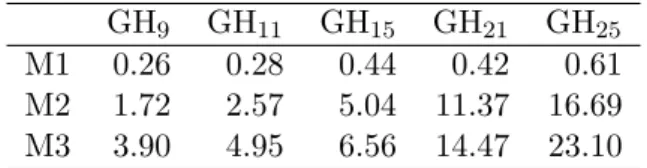
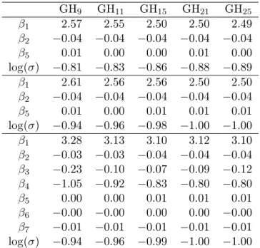
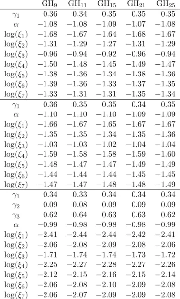
An important aspect for the success of the optimization procedure described above in ap-proximating the true maximum likelihood estimates, is the accuracy of the Gauss-Hermite quadrature rule. As it is known from the mixed models literature (Pinheiro and Bates 1995), the choice of the number of quadrature points may influence the parameter estimates, stan-dard errors and the log-likelihood value. Thus, it is typically advisable to investigate the fit of the model with an increasing number of quadrature points and/or consider the adap-tive Gauss-Hermite rule that appropriately re-scales the quadrature points in the area where the integrand has its main mass. It is obvious that both these procedures increase substan-tially the computing time required to fit joint models. However, fortunately, we can decrease computational intensity without sacrificing too much precision by taking into advantage the information we have available from the linear mixed effects model fit that is provided as first
argument in jointModel(). To illustrate how this can be achieved, we first compare the
logarithm of the integrands in the linear mixed effects and joint models, given respectively as: logp(yi, bi;θ) =
ni
X
j=1
logp{yi(tij)|bi;θy}+ logp(bi;θb),
logp(Ti, δi, yi, bi;θ) =
ni
X
j=1
Following an argument similar to the one raised in Step 2 of the Monte Carlo scheme of Section2.4, we observe that the leading term in both integrands is the density p(yi |bi;θy) =
Q
jp{yi(tij) | bi;θy} (Rizopoulos et al. 2008). This means that, especially as ni increases, we expect both integrands to have their main mass around the same location. The fitting
algorithms behind jointModel() take this information into account and scale the
Gauss-Hermite quadrature points accordingly. This procedure shares similarities with the adaptive Gauss-Hermite rule, but we implement it only once, at the start of the optimization, and we do not further update the quadrature points afterwards. Based on empirical evidence, we have observed that even though we do not update the quadrature points at each iteration of the optimization algorithm (as in the adaptive Gauss-Hermite rule), this procedure performs very well in practice. The computational advantages are twofold: first, we can use fewer quadrature points than we would have used in the standard (i.e., non-adaptive) Gauss-Hermite rule, and second, we avoid the computationally demanding relocation of the quadrature points at each iteration of the adaptive Gauss-Hermite rule. A numerical study regarding the performance of this approach and further discussion is provided in AppendixA.
4. Analysis of a real data example using
JM
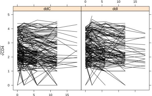
As an illustrative example of joint modelling we consider a longitudinal study on 467 HIV infected patients who had failed or were intolerant of zidovudine therapy. The aim of the study was to compare the efficacy and safety of two alternative antiretroviral drugs, namely didanosine (ddI) and zalcitabine (ddC). Patients were randomly assigned to receive either ddI or ddC, and CD4 cell counts were recorded at study entry, where randomization took place, as well as 2, 6, 12, and 18 months thereafter. By the end of the study 188 patients had died,
resulting in 59.7% censoring. More details about this data set can be found in Goldman,
Carlin, Crane, Launer, Korvick, Deyton, and Abrams (1996). Our main research question here is to test for a treatment effect on survival after adjusting for the CD4 cell count. Due to the fact that the CD4 cell count measurements are in fact the output of a stochastic process generated by the patients and is only available at the specific visit times the patients came to the study center, it constitutes a typical example of time-dependent covariate measured intermittently and with error for which joint modelling is required.
The longitudinal and survival information for these patients is available in JM in the data
frames aids and aids.id, respectively. The CD4 cell counts are known to exhibit right
skewed shapes of distribution, and therefore, for the remainder of this analysis we will work with the square root of the CD4 cell values. As a descriptive analysis we present in Figure 1
the subject-specific longitudinal profiles and the Kaplan-Meier estimate for the time-to-death:
R> library("JM") R> library("lattice")
R> xyplot(sqrt(CD4) ~ obstime | drug, group = patient, data = aids,
+ xlab = "Months", ylab = expression(sqrt("CD4")), col = 1, type = "l") R> plot(survfit(Surv(Time, death) ~ drug, data = aids.id), conf.int = FALSE, + mark.time = TRUE, col = c("black", "red"), lty = 1:2,
+ ylab = "Survival", xlab = "Months")
R> legend("topright", c("ddC", "ddI"), lty = 1:2, col = c("black", "red"), + bty = "n")
Months CD4 0 1 2 3 4 5 0 5 10 15 ddC 0 5 10 15 ddI
Figure 1: Subject-specific evolutions in time of the square root of the CD4 cell count mea-surements, separately for ddC and ddI.
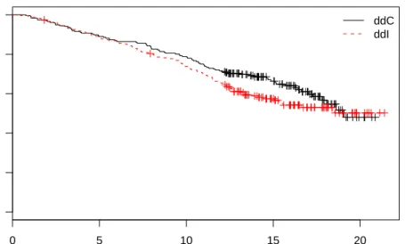
We observe that in both groups patients show similar variability in their longitudinal profiles, whereas from the Kaplan-Meier estimate in Figure2it seems that the ddC group has slightly higher survival than the ddI group after the six month of follow-up.
To illustrate the virtues of the joint modelling approach, we will first start with a ‘naive’ analysis, in which we ignore the special characteristics of the CD4 cell counts and we fit a Cox model that includes the treatment indicator and CD4 as an ordinary time-dependent covariate (i.e., ignoring the measurement error). To fit this models we will use the standard counting process form of the Cox model:
R> td.Cox <- coxph(Surv(start, stop, event) ~ drug + sqrt(CD4), data = aids) R> summary(td.Cox)
Call:
coxph(formula = Surv(start, stop, event) ~ drug + sqrt(CD4), data = aids)
n= 1405
coef exp(coef) se(coef) z Pr(>|z|)
drugddI 0.32678 1.38650 0.14708 2.222 0.0263 *
sqrt(CD4) -0.72302 0.48528 0.07997 -9.042 <2e-16 ***
0 5 10 15 20 0.0 0.2 0.4 0.6 0.8 1.0 Months Sur viv al ddC ddI
Figure 2: Kaplan-Meier estimates of the probability of survival for the ddC and ddI treatment groups.
exp(coef) exp(-coef) lower .95 upper .95
drugddI 1.3865 0.7212 1.0393 1.8498
sqrt(CD4) 0.4853 2.0606 0.4149 0.5676
Rsquare= 0.059 (max possible= 0.786 )
Likelihood ratio test= 86.14 on 2 df, p=0
Wald test = 83.51 on 2 df, p=0
Score (logrank) test = 83.25 on 2 df, p=0
Variablesstartand stop denote the limits of the time intervals between visits in the study center, andeventtakes the value 1 when a patient died; for more details we refer toTherneau and Grambsch(2000, Section 3.7).
We observe that after adjusting for the square root of CD4 count in the Cox model, there is not a strong evidence for a treatment effect. We proceed by specifying and fitting a joint model that explicitly postulates a linear mixed effects model for the CD4 cell counts. In particular, taking advantage of the randomization set-up of the study, we include in the fixed-effects part of the longitudinal submodel the main effect of time and the interaction of treatment with time. In the random-effects design matrix we include an intercept and a time term. For the survival submodel and similarly to the Cox model above, we include as a time-independent covariate the treatment effect, and as time-dependent one the true underlying effect of CD4 cell count as estimated from the longitudinal model. The baseline risk function is assumed piecewise constant with six knots placed at equally spaced percentiles of the observed event
times. In particular, {v1, . . . , vQ−1} in (15) are specified as quantile(Time, seq(0, 1,
length = Q + 1))[-c(1, Q + 1)], where Q equals seven, and Time is the numeric vector
that contains the observed event times Ti, (i = 1, . . . , n). In order to fit this joint model we need first to fit separately the linear mixed effects and Cox models, and then supply the returned objects as main arguments injointModel(). More specifically, the joint model fitted
byjointModel()has exactly the same structure for the longitudinal and survival submodels
as these two separately fitted models, with the addition that in the survival submodel the effect of the estimated ‘true’ longitudinal outcomemi(t) is included in the linear predictor.
Furthermore, due to the fact that jointModel() extracts all the required information from
these two objects (e.g., response vectors, design matrices, etc.), in the call to coxph() we
need to specify the argument x = TRUE in order for the design matrix of the Cox model to
be included in the returned object, i.e.,
R> fitLME <- lme(sqrt(CD4) ~ obstime + obstime:drug, + random = ~ obstime | patient, data = aids)
R> fitSURV <- coxph(Surv(Time, death) ~ drug, data = aids.id, x = TRUE) R> fit.JM <- jointModel(fitLME, fitSURV, timeVar = "obstime",
+ method = "piecewise-PH-GH") R> summary(fit.JM)
Call:
jointModel(lmeObject = fitLME, survObject = fitSURV, timeVar = "obstime", method = "piecewise-PH-GH")
Data Descriptives:
Longitudinal Process Event Process
Number of Observations: 1405 Number of Events: 188 (40.3%)
Number of Groups: 467 Joint Model Summary:
Longitudinal Process: linear mixed effects model
Event Process: Relative risk model with piecewise-constant baseline risk function (knots at: 6.2, 11.1, 12.5, 13.9, 16, 17.8)
log.Lik AIC BIC
-2107.647 4247.295 4313.636 Variance Components: StdDev Corr (Intercept) 0.8660 (Intr) obstime 0.0388 0.0681 Residual 0.3754 Coefficients: Longitudinal Process
Value Std.Err z-value p-value
obstime -0.0423 0.0046 -9.1932 <0.0001
obstime:drugddI 0.0051 0.0065 0.7819 0.4343
Event Process
Value Std.Err z-value p-value
drugddI 0.3510 0.1537 2.2829 0.0224 Assoct -1.1019 0.1180 -9.3399 <0.0001 log(xi.1) -1.6483 0.2499 -6.5973 log(xi.2) -1.3388 0.2394 -5.5913 log(xi.3) -1.0226 0.2861 -3.5736 log(xi.4) -1.5795 0.3736 -4.2282 log(xi.5) -1.4716 0.3500 -4.2050 log(xi.6) -1.4375 0.4282 -3.3567 log(xi.7) -1.4767 0.5454 -2.7077 Integration: method: Gauss-Hermite quadrature points: 15 Optimization: Convergence: 0
The main argumenttimeVar of jointModel() is used to specify the name of the time
vari-able in the linear mixed effects model, which is required for the computation ofmi(t). The
summary() method returns a detailed output, including among others the parameter
esti-mates, their standard errors, and asymptotic Wald tests for both the longitudinal and sur-vival submodels. In the results of the event process the parameter labeled‘Assoct’is in fact parameterα in (1) that measures the effect of mi(t) (i.e., in our case of the true square root CD4 cell count) in the risk for death. The parametersxiare the ξq (q = 1, . . . ,7) parameters for the piecewise constant baseline risk function in (15). A comparison between the standard time-dependent Cox model with the joint model reveals some interesting features. In par-ticular, we observe that the regression coefficient for ddI is larger in magnitude in the joint model, which results in a slightly stronger treatment effect. Much stronger bias is observed for the effect of the CD4 cell count, with estimated regression coefficient−0.72 for the time-dependent Cox model and −1.10 for the joint model. As an alternative to the Wald test, a likelihood ratio test (LRT) can be also used to test for a treatment effect. To perform this test we need to fit the joint model under the null hypothesis of no treatment effect in the
survival submodel, and then use theanova()method:
R> fitSURV2 <- coxph(Surv(Time, death) ~ 1, data = aids.id, x = TRUE) R> fit.JM2 <- jointModel(fitLME, fitSURV2, timeVar = "obstime",
+ method = "piecewise-PH-GH") R> anova(fit.JM2, fit.JM)
AIC BIC log.Lik LRT df p.value
fit.JM2 4250.53 4312.72 -2110.26
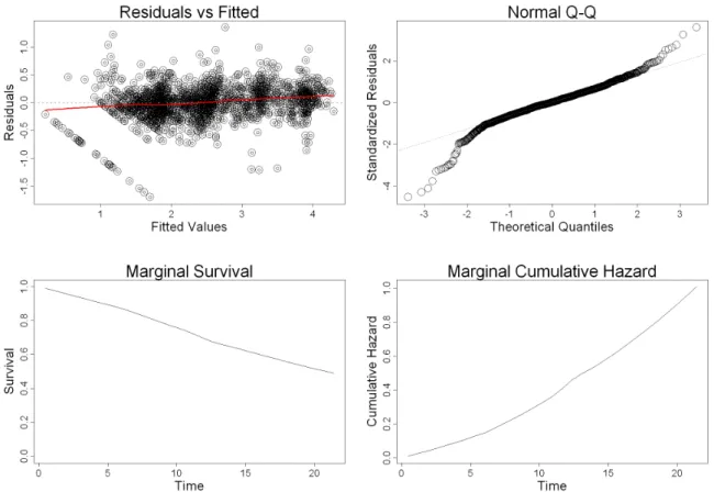
Figure 3: Diagnostic plots for the fitted joint model. The top-left panel depicts the subject-specific residuals for the longitudinal process versus their corresponding fitted values. The top-right panel depicts the normal Q-Q plot of the standardized subject-specific residuals for the longitudinal process. The bottom-left depicts an estimate of the marginal survival function for the event process. The bottom-right depicts an estimate of the marginal cumulative risk function for the event process.
We arrive at the same conclusion with an almost identical p value to the Wald test. The
anova()method for class jointModelaccepts as arguments two fitted joint models, with the
first one always being the model under the null.
We proceed by checking the fit of the model using residuals plots. As it is standard inR, the residuals and fitted values can be extracted from a fitted model using the generic functions
residuals() and fitted(), respectively. For joint models fitted by jointModel()we have
several kinds of residuals and fitted values depending on the outcome (i.e., longitudinal or time-to-event) and the level of focus (i.e., marginalized over the subjects or subject-specific)
– for more details we refer to Appendix B. Some model diagnostics are directly available
by calling the plot() method for jointModel objects – for our fitted joint model this is
illustrated in Figure 3.
R> par(mfrow = c(2, 2)) R> plot(fit.JM)
calcu-lated according to the formula S(t) = Z Si(t|bi; ˆθ)p(bi; ˆθ)dbi≈n−1 X i Si(t|ˆbi; ˆθ),
where ˆbidenotes the empirical Bayes estimates for the random effects. The estimated marginal cumulative risk function is simply calculated asHi(t) =−logS(t). Additional residuals plots can be easily computed by first calculating the specific type of residuals of interest, and then plotting them against the corresponding fitted values or covariates. For example, the
code below produces Figure 4 that contains the plots of the standardized subject-specific
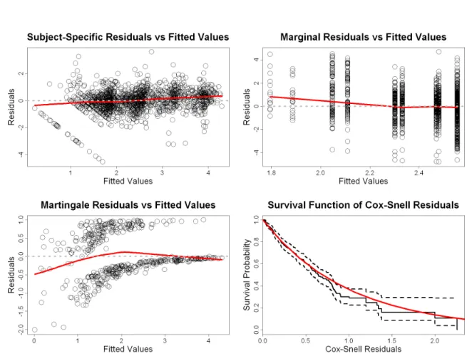
and standardized marginal residuals versus fitted values for the longitudinal process, and the martingale residuals versus ˆmi(Ti) and the Kaplan-Meier estimate of the Cox-Snell residuals for the event process (functionplotResid()used to produce the following residuals plots can
be found in AppendixC).
R> par(mfrow = c(2, 2))
R> resSubY <- residuals(fit.JM, process = "Longitudinal", + type = "stand-Subject")
R> fitSubY <- fitted(fit.JM, process = "Longitudinal", type = "Subject") R> plotResid(fitSubY, resSubY, xlab = "Fitted Values", ylab = "Residuals", + main = "Subject-Specific Residuals vs Fitted Values")
R> resMargY <- residuals(fit.JM, process = "Longitudinal", + type = "stand-Marginal")
R> fitMargY <- fitted(fit.JM, process = "Longitudinal", type = "Marginal") R> plotResid(fitMargY, resMargY, xlab = "Fitted Values", ylab = "Residuals", + main = "Marginal Residuals vs Fitted Values")
R> resMartT <- residuals(fit.JM, process = "Event", type = "Martingale") R> fitSubY <- fitted(fit.JM, process = "Longitudinal", type = "EventTime") R> plotResid(fitSubY, resMartT, xlab = "Fitted Values", ylab = "Residuals", + main = "Martingale Residuals vs Fitted Values")
R> resCST <- residuals(fit.JM, process = "Event", type = "CoxSnell") R> sfit <- survfit(Surv(resCST, death) ~ 1, data = aids.id)
R> plot(sfit, mark.time = FALSE, conf.int = TRUE, lty = 1:2, + xlab = "Cox-Snell Residuals", ylab = "Survival Probability", + main = "Survival Function of Cox-Snell Residuals")
R> curve(exp(-x), from = 0, to = max(aids.id$Time), add = TRUE, + col = "red", lwd = 2)
We observe that the fitted loess curve in the plot of the standardized marginal residuals versus the fitted values shows a systematic trend with more positive residuals for small fitted values.
However, as mentioned in Section 2.3, due to the nonrandom dropout in the longitudinal
outcome caused by the occurrence of events, conclusions from residuals based on the observed data alone should be extracted with caution. For instance, in our example small numbers of
Figure 4: Diagnostic plots for the fitted joint model. The dashed lines in bottom-right panel denote the 95% confidence intervals for the Kaplan-Meier estimate of the Cox-Snell residuals. CD4 cell counts indicate a worsening of patients’ condition resulting in higher death rates (i.e., dropout). Thus, the residuals corresponding to small fitted values are only based on patients with a ‘good’ health condition, which results in the systematic trend. To take dropout into account we will use the multiply-imputed residuals introduced in Section2.3. The simulation
scheme described in Section 2.3 is available via the residuals() method for jointModel
objects, and can be invoked using the logical argument MI. As an illustration, we calculate the multiply-imputed standardized marginal residuals (we set the seed for reproducibility):
R> set.seed(123)
R> res.MI <- residuals(fit.JM, process = "Longitudinal", + type = "stand-Marginal", MI = TRUE)
R> fitMargY.miss <- res.MI$fitted.valsM R> resMargY.miss <- res.MI$resid.valsM
Contrary to the standard call toresiduals() that returns a numeric vector of residuals (as illustrated above), setting MI to TRUE returns a list with several components useful in the further processing of the multiply-imputed residuals. The two components that we extract here are the fitted values and the multiply-imputed standardized marginal residuals that correspond to ymi , as defined in Section 2.3. Object fitMargY.miss is a numeric vector,
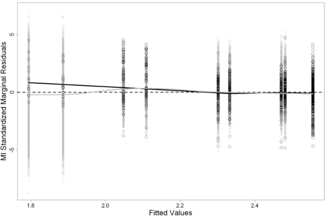
Figure 5: Observed standardized marginal residuals (black circles), augmented with all the
multiply imputed residuals produced by theL= 50 imputations (grey points). The
superim-posed solid lines represent a loess fit based only on the observed residuals (black line), and a weighted loess fit based on all residuals (grey line).
the residuals based on the multiple-imputations for ymi (default is 50 multiple-imputations;
this is controlled by argument M of residuals()). The following code produces Figure 5
that depicts the multiply-imputed residuals together with the observed residuals versus their corresponding fitted values:
R> M <- ncol(resMargY.miss)
R> resMargY.MI <- c(resMargY, resMargY.miss)
R> fitMargY.MI <- c(fitMargY, rep(fitMargY.miss, M))
R> plot(range(fitMargY.MI), range(resMargY.MI), type = "n",
+ xlab = "Fitted Values", ylab = "MI Standardized Marginal Residuals") R> abline(h = 0, lty = 2)
R> points(rep(fitMargY.miss, M), resMargY.miss, cex = 0.5, col = "grey") R> points(fitMargY, resMargY)
The black loess curve in Figure5is in fact the same curve as in the top-right panel of Figure4
and is produced by
However, to produce the grey loess curve, which describes the relationship between the com-plete residuals (i.e., the multiply-imputed residuals together with the observed residuals) versus their corresponding fitted values, some extra steps are required. In particular, we need to take into account that for each of the time points the i-th subject did not appear in the
study center we have M = 50 multiply-imputed residuals, whereas for the times that he did
appear we only have one. Thus, in the calculation of the loess curve we will use case weights with the value 1 for the observed residuals and 1/M = 1/50 = 0.02 for the multiply-imputed ones, i.e.,
R> dat.resid <- data.frame( + resid = resMargY.MI, + fitted = fitMargY.MI,
+ weight = c(rep(1, length(resMargY)), rep(1/M, length(resMargY.miss))) + )
R> fit.loess <- loess(resid ~ fitted, data = dat.resid, weights = weight) R> nd <- data.frame(fitted = seq(min(fitMargY.MI), max(fitMargY.MI), + length.out = 100))
R> prd.loess <- predict(fit.loess, nd)
R> lines(nd$fitted, prd.loess, col = "grey", lwd = 2)
A comparison between the two loess smoothers reveals that indeed the systematic trends that were present in the residual plots based on the observed data alone are mainly attributed to the nonrandom dropout and not to a model lack-of-fit.
Following we will focus on the calculation of expected survival probabilities. The Monte
Carlo scheme of Section 2.4 is implemented in function survfitJM() that accepts as main
arguments a fitted joint model, and a data frame that contains the longitudinal and covariate information for the subjects for which we wish to calculate the predicted survival probabilities. Here we compute πi(u | t) for four patients in the data set who have not died by the time of loss to follow-up, using L = 200 Monte Carlo samples (as previously, we set the seed for reproducibility):
R> set.seed(123)
R> ND <- aids[aids$patient %in% c("7", "15", "117", "303"), ] R> predSurv <- survfitJM(fit.JM, newdata = ND, idVar = "patient", + last.time = "Time")
R> predSurv
Prediction of Conditional Probabilities for Event based on 200 replications
$`7`
times Mean Median Lower Upper
1 14.6962 0.9863 0.9879 0.9696 0.9945 2 15.3147 0.9629 0.9673 0.9177 0.9853 3 15.9332 0.9393 0.9465 0.8655 0.9761 4 16.5518 0.9136 0.9209 0.8110 0.9651 5 17.1703 0.8877 0.8952 0.7628 0.9516 6 17.7888 0.8617 0.8715 0.7025 0.9421
7 18.4074 0.8359 0.8523 0.6502 0.9308 8 19.0259 0.8103 0.8302 0.6115 0.9245 9 19.6444 0.7849 0.8091 0.5475 0.9167 10 20.2629 0.7597 0.7897 0.4852 0.9107 11 20.8815 0.7349 0.7643 0.4159 0.8978 12 21.5000 0.7105 0.7425 0.3741 0.8905 ...
By defaultsurvfitJM()computesπi(u|t) at a set of equally spaced time points, produced by a regular sequence of length 35 starting from the minimum observed event time to the
max-imum observed event time (i.e., seq(min(Time), max(Time) + 0.1, length.out = 35));
this default choice can be changed by specifying in argumentsurvTimes a numeric vector of
time points at whichπi(u|t) is to be computed. We should note however thatsurvfitJM() actually computesπi(u|t) for each subject for the time points that are later than the time of the last available longitudinal measurement (e.g., if a subject had provided longitudinal mea-surements up to timet,survfitJM()will computeπi(u|t) for allu > t). This is because for the time points that are earlier than the time of the last available longitudinal measurement we know that this subject was alive and therefore πi(u | t) = 1 (see also Section 2.4). In addition, if the last time point at which a subject was still alive is later than the time point of his last available longitudinal measurement, then this can be specified via the optional argumentlast.time; for instance, in our example we specifylast.time = "Time"since we know that all four patients were still alive at the censoring time, which is given by the vari-ableTime in data frame ND. The printed outputsurvfitJM() is rather self-explanatory – to avoid including here the whole lengthy output for all four patients, we only show the results for Patient 7. This patient provided CD4 cell count measurements up to 12 months from randomization and he was lost to follow-up after 14.3 months. He has 75% probability of surviving more than 21.4 months (which is the largest recorded follow-up time) with a 95% pointwise confidence interval ranging from 38% to 89%. The estimatedπi(u|t)’s can also be plotted using theplot() method for objects of classsurvfitJM. In particular, a simple call
toplot() produces Figure 6:
R> par(mfrow = c(2, 2))
R> plot(predSurv, conf.int = TRUE)
Furthermore, thefunargument of theplot()method can be used to produce various
trans-formations of πi(u | t). For instance, the following code includes in Figure 7 the plots of expected survival, natural logarithm of expected survival, and expected cumulative risk
R> par(mfrow = c(2, 2))
R> plot(predSurv, which = "7", conf.int = TRUE)
R> plot(predSurv, which = "7", conf.int = TRUE, fun = log, + ylab = "log Survival")
R> plot(predSurv, which = "7", conf.int = TRUE, fun = function (x) -log(x), + ylab = "Cumulative Risk")
An additional option provided by the plot() method for survfitJM objects, is to include
in the same figure the estimated πi(u |t) and the longitudinal information for each patient. This is illustrated for Patient 7 in Figure8 that is produced with following piece of code:
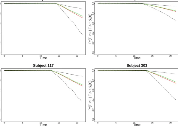
0 5 10 15 20 0.0 0.2 0.4 0.6 0.8 1.0 Subject 7 Time Pr( Ti ≥ u | Ti > t, y~i ( t ) ) 0 5 10 15 20 0.0 0.2 0.4 0.6 0.8 1.0 Subject 15 Time Pr( Ti ≥ u | Ti > t, y~i ( t ) ) 0 5 10 15 20 0.0 0.2 0.4 0.6 0.8 1.0 Subject 117 Time Pr( Ti ≥ u | Ti > t, y~i ( t ) ) 0 5 10 15 20 0.0 0.2 0.4 0.6 0.8 1.0 Subject 303 Time Pr( Ti ≥ u | Ti > t, y~i ( t ) )
Figure 6: Predicted probabilities of survival for four patients who have not died by the end of the study, based on 200 Monte Carlo samples. The red and greed solid lines depict the mean and median, respectively, of πi(u |t) over the Monte Carlo samples. The black dashed lines depict a 95% pointwise confidence intervals based on the quantiles ofπi(u|t) over the Monte Carlo samples.
R> plot(predSurv, conf.int = TRUE, estimator = "median", which = "7", + include.y = TRUE)
Theestimator argument specifies which estimate of πi(u |t) to plot (i.e., mean, median or
both), argumentwhich can be used to specify for which specific subject we want to produce
the plot, and logical argument include.y adds in the same figure the scatter plot of the
longitudinal responses of this subject versus time. This figure is useful in investigating whether specific longitudinal profiles result in steeper survival curves, which could be insightful for the mechanisms that underly the medical condition under study.
Finally, to make the connection with the missing data framework we can compare the results of the linear mixed effects model ignoring the dropout process with the results of the longitudinal submodel from the joint model fit:
R> summary(fitLME)
Linear mixed-effects model fit by REML Data: aids
0 5 10 15 20 0.0 0.2 0.4 0.6 0.8 1.0 Subject 7 Time Pr( Ti ≥ u | Ti > t, y~i ( t ) ) 0 5 10 15 20 −1.0 −0.8 −0.6 −0.4 −0.2 0.0 Subject 7 Time log Sur viv al 0 5 10 15 20 0.0 0.2 0.4 0.6 0.8 1.0 Subject 7 Time Cum ulativ e Risk
Figure 7: Transformations of the predicted survival probabilities for death for Patient 7,
based on 200 Monte Carlo samples. The green solid line depicts the median ofπi(u|t) over the Monte Carlo samples. The black dashed lines depict a 95% pointwise confidence interval.
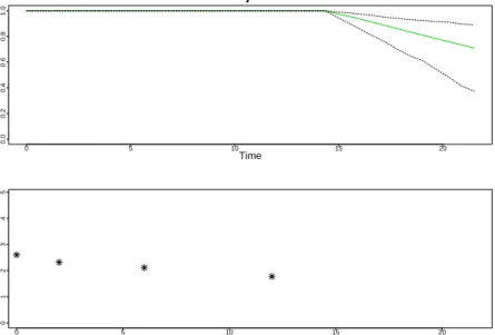
0 5 10 15 20 0.0 0.2 0.4 0.6 0.8 1.0 Subject 7 Time Pr( Ti ≥ u | Ti > t, y~i ( t ) ) 0 5 10 15 20 0 1 2 3 4 5 Time Longitudinal Outcome
Figure 8: Predicted survival probabilities for Patient 7 (top panel) including also his available
longitudinal √CD4 cell counts measurements (bottom panel), based on 200 Monte Carlo
samples. The green solid line depicts the median ofπi(u |t) over the Monte Carlo samples. The black dashed lines depict a 95% pointwise confidence interval.
AIC BIC logLik 2699.069 2735.789 -1342.535 Random effects:
Formula: ~obstime | patient
Structure: General positive-definite, Log-Cholesky parametrization
StdDev Corr
(Intercept) 0.87143264 (Intr)
obstime 0.03617033 -0.015
Residual 0.36844785
Fixed effects: sqrt(CD4) ~ obstime + obstime:drug
Value Std.Error DF t-value p-value
(Intercept) 2.5118005 0.04258901 936 58.97766 0.0000 obstime -0.0375070 0.00440225 936 -8.51997 0.0000 obstime:drugddI 0.0082141 0.00632277 936 1.29912 0.1942 Correlation: (Intr) obstim obstime -0.118 obstime:drugddI 0.000 -0.687 ...
We observe a rather very small sensitivity, which is more easily noticeable by comparing the
parameter estimates divided by their corresponding standard errors (i.e., z-value column
in the results of the joint model fit and t-value column in the results of the linear mixed
model fit). However, note that we have relaxed the MAR assumption only towards the
MNAR mechanism implied by joint models (9) – we cannot definitely claim that there are no sensitivity issues.
5. Extra features and extensions
In this article we have illustrated the capabilities of package JM for the joint modelling of longitudinal and time-to-event data using shared parameter models. These models are appli-cable when either we wish to account for the effect of a time-dependent covariate measured with error in a survival analysis context or when we wish to correct for nonrandom dropout in the analysis of longitudinal outcomes.
Even though in Section 4 we have focused on joint models with a relative risk submodel
with a piecewise constant baseline risk function for the event outcome, JM offers several
other options for the survival submodel as described in Section3.1. Moreover, formethod =
"weibull-PH-GH"andmethod = "weibull-AFT-GH"thescaleWBargument ofjointModel()
can be used to fix the scale parameter of the Weibull hazard function to a specific value (e.g., settingscaleWB = 1, the Weibull hazard reduces to the exponential hazard). In addition, for
method = "spline-PH-GH", it is also possible to include stratification factors, i.e., different
different levels of categorical variable. To fit such a stratified joint model the user needs to include the stratification factors in the definition of the survival model, which must only
be a Cox model. For instance, for the AIDS data set analyzed in Section 4, the following
code includes as a stratification factor variable that distinguishes between patients who were intolerant or had failure in the standard treatment for AIDS:
R> fitSURV3 <- coxph(Surv(Time, death) ~ drug + strata(AZT), data = aids.id, + x = TRUE)
R> fit.JM3 <- jointModel(fitLME, fitSURV3, timeVar = "obstime", + method = "spline-PH-GH")
The supporting functionwald.strata() can be used to test for equality of the spline coeffi-cients across strata with a Wald test. Furthermore, for all types of joint models available in JMit is possible to postulate a lag effect for the longitudinal time-dependent covariate, that is
hi(t| Mi(t), wi) =h0(t) exp[γ>wi+αmi{min(t−k,0)}],
where k > 0. This is controlled by the argument lag of jointModel() that defaults to 0.
Finally, a further issue in the calculation of the multiple-imputation residuals is the nature of the visiting process (i.e., the stochastic mechanism that generates the time points at which
the longitudinal measurements are collected). In particular, in the AIDS study patients
were supposed to provide CD4 cell count measurements at fixed follow-up times. However, in observational studies and in some randomized trials, the time points at which the longitudinal measurements are taken are not fixed by design but rather determined by the physician or even the patients themselves. The possibility of random visit times complicates the methodology presented in Section 2.3 due to the fact that the time points at which the i-th subject was
supposed to provide measurements after the observed event time Ti are not available, and
thus the corresponding rowsx>i (tij) andz>i (tij), fortij ≥Ti, of the design matricesXi andZi, respectively, required in Step 3 of the simulation scheme of Section 2.3, cannot be specified. To overcome this problemJMoffers the option to model the visiting process (using a Weibull
model with a Gamma frailty implemented in function weibull.frailty()), and use this
visiting model to simulate future visit times for each individual. An example of this procedure as well as up-to-date information regarding the current and future features of the package, and
R scripts, with detailed analysis of real data sets illustrating these features, can be found in
theRwiki page ofJM, accessible athttp://rwiki.sciviews.org/doku.php?id=packages:
cran:jm.
PackageJMis still under active development. Future plans include among others, the handling of interval censored and grouped survival data, different types of parameterizations for the survival model, and the implementation of the fully exponential Laplace approximation for the other types of survival models available injointModel().
References
Allignol A, Latouche A (2010). CRAN Task View: Survival Analysis. Version 2010-05-26,
Bates D, Maechler M (2010).lme4: Linear Mixed-Effects Models UsingS4 Classes.Rpackage
version 0.999375-34, URLhttp://CRAN.R-project.org/package=lme4.
Brown E, Ibrahim J (2003). “A Bayesian Semiparametric Joint Hierarchical Model for Lon-gitudinal and Survival Data.”Biometrics,59, 221–228.
Brown E, Ibrahim J, DeGruttola V (2005). “A Flexible B-Spline Model for Multiple Longi-tudinal Biomarkers and Survival.”Biometrics,61, 64–73.
Chi YY, Ibrahim J (2006). “Joint Models for Multivariate Longitudinal and Multivariate Survival Data.”Biometrics,62, 432–445.
Cox D, Hinkley D (1974). Theoretical Statistics. Chapman & Hall, London. Cox D, Oakes D (1984). Analysis of Survival Data. Chapman & Hall, London.
Ding J, Wang JL (2008). “Modeling Longitudinal Data with Nonparametric Multiplicative Random Effects Jointly with Survival Data.”Biometrics,64, 546–556.
Follmann D, Wu M (1995). “An Approximate Generalized Linear Model with Random Effects for Informative Missing Data.”Biometrics,51, 151–168.
Goldman A, Carlin B, Crane L, Launer C, Korvick J, Deyton L, Abrams D (1996). “Response of CD4+ and Clinical Consequences to Treatment Using ddI or ddC in Patients with
Advanced HIV Infection.”Journal of Acquired Immune Deficiency Syndromes and Human
Retrovirology,11, 161–169.
Guo X, Carlin B (2004). “Separate and Joint Modeling of Longitudinal and Event Time Data
using Standard Computer Packages.”The American Statistician,58, 16–24.
Harrell F (2001).Regression Modeling Strategies: With Applications to Linear Models, Logistic Regression, and Survival Analysis. Springer-Verlag, New York.
Henderson R, Diggle P, Dobson A (2000). “Joint Modelling of Longitudinal Measurements and Event Time Data.”Biostatistics,1, 465–480.
Hsieh F, Tseng YK, Wang JL (2006). “Joint Modeling of Survival and Longitudinal Data: Likelihood Approach Revisited.”Biometrics,62, 1037–1043.
Kalbfleisch J, Prentice R (2002). The Statistical Analysis of Failure Time Data. 2nd edition. John Wiley & Sons, New York.
Lange K (2004). Optimization. Springer-Verlag, New York.
Little R, Rubin D (2002). Statistical Analysis with Missing Data. 2nd edition. John Wiley & Sons, New York.
Nobre J, Singer J (2007). “Residuals Analysis for Linear Mixed Models.”Biometrical Journal,
6, 863–875.
Pinheiro J, Bates D (1995). “Approximations to the Log-Likelihood Function in the Nonlinear Mixed-Effects Model.”Journal of Computational and Graphical Statistics,4, 12–35.
Pinheiro J, Bates D, DebRoy S, Sarkar D, R Development Core Team (2009). nlme: Linear and Nonlinear Mixed Effects Models. R package version 3.1-96, URL http: //CRAN.R-project.org/package=nlme.
RDevelopment Core Team (2010).R: A Language and Environment for Statistical Computing.
RFoundation for Statistical Computing, Vienna, Austria. ISBN 3-900051-07-0, URLhttp:
//www.R-project.org/.
Rizopoulos D, Verbeke G, Lesaffre E (2009). “Fully Exponential Laplace Approximations for
the Joint Modelling of Survival and Longitudinal Data.” Journal of the Royal Statistical
Society B,71, 637–654.
Rizopoulos D, Verbeke G, Molenberghs G (2008). “Shared Parameter Models under Random Effects Misspecification.”Biometrika,95, 63–74.
Rizopoulos D, Verbeke G, Molenberghs G (2010). “Multiple-Imputation-Based Residuals and Diagnostic Plots for Joint Models of Longitudinal and Survival Outcomes.”Biometrics,66, 20–29.
Song X, Davidian M, Tsiatis A (2002). “A Semiparametric Likelihood Approach to Joint
Modeling of Longitudinal and Time-to-Event Data.”Biometrics,58, 742–753.
Therneau T, Grambsch P (2000).Modeling Survival Data: Extending the Cox Model.
Springer-Verlag, New York.
Therneau T, Lumley T (2009). survival: Survival Analysis Including Penalised Likelihood.
Rpackage version 2.35-8, URLhttp://CRAN.R-project.org/package=survival.
Tseng YK, Hsieh F, Wang JL (2005). “Joint Modelling of Accelerated Failure Time and Longitudinal Data.”Biometrika,92, 587–603.
Tsiatis A, Davidian M (2001). “A Semiparametric Estimator for the Proportional Hazards
Model with Longitudinal Covariates Measured with Error.”Biometrika,88, 447–458.
Tsiatis A, Davidian M (2004). “Joint Modeling of Longitudinal and Time-to-Event Data: An Overview.”Statistica Sinica,14, 809–834.
Verbeke G, Molenberghs G (2000). Linear Mixed Models for Longitudinal Data.
Springer-Verlag, New York.
Wang Y, Taylor J (2001). “Jointly Modeling Longitudinal and Event Time Data with
Ap-plication to Acquired Immunodeficiency Syndrome.” Journal of the American Statistical
Association,96, 895–905.
Wulfsohn M, Tsiatis A (1997). “A Joint Model for Survival and Longitudinal Data Measured with Error.” Biometrics,53, 330–339.
Xu J, Zeger S (2001). “Joint Analysis of Longitudinal Data Comprising Repeated Measures and Times to Events.”Applied Statistics,50, 375–387.
Yu M, Law N, Taylor J, Sandler H (2004). “Joint Longitudinal-Survival-Cure Models and their Application to Prostate Cancer.”Statistica Sinica,14, 835–832.