Debt consolidation with long-term debt
Alexander Scheer∗
This version: April 2015
Abstract
The Great Recession has sent debt levels to a post-WWII high for several advanced economies, reviving the discussion of fiscal consolidation. This paper assesses the macroe-conomic implications of tax-based versus spending-based consolidation within the frame-work of a New Keynesian model with long term government debt. Three results stand out: First, tax-based consolidations are inflationary whereas spending-based ones are deflation-ary. Second, the net benefits of inflation increase in the average maturity of outstanding debt: inflation revalues debt more efficiently, while distortions due to price dispersion remain unaffected. Third, as a result, tax-based consolidations can become superior to spending cuts if the average maturity is high enough. Quantitatively, the threshold is two years for US data in 2013. The previous mechanism illustrates the importance of inflation in the consolidation process, even if raising its target rate is considered not to be an option.
Keywords: Consolidation, Long term debt, Monetary policy, Fiscal policy, Inflation,
New-Keynesian models
JEL-Codes: H63, E63
∗
University of Bonn, Adenauerallee 24-42, 53113 Bonn, Germany. Email: alexander.scheer@uni-bonn.de. The first version is from April 2014. I thank Gernot J. M¨uller, J¨urgen von Hagen, Klaus Adam, Stefania Albanesi, Francesco Bianchi, Filippo Brutti and Michael Kumhof for valuable comments and discussions as well as seminar participants at Bonn, Durham, Thessaloniki, Dresden and Warwick. I also thank the German Science Foundation (DFG) for financial support under the Research Training Group 1707.
1
Introduction
The Great Recession has sent government debt levels to a post-WWII high for several ad-vanced economies. The increase in debt was driven by a sharp reduction in GDP coupled with discretionary fiscal stimulus and financial sector support, see IMF (2011). Debt to GDP has increased by roughly 37 percentage points from 2007 to 2014 for 19 OECD countries. Figure 1 depicts the path of debt ratios for the G7 countries and table 1 the respective change from 2007-2014. As one can see debt levels still remain high and, except for Germany and Canada, do not seem to return to pre-crisis levels.
These elevated debt to GDP ratios have revived discussions on optimal debt levels and possible ways of consolidation. Although the literature does not agree on a specific level of debt (see the next section), it seems that the current ratios are not considered as optimal. A natural question arising is how to reduce that debt in the least distortionary way - that is when to reduce it and which instruments to use. Most of the theoretical literature focuses on the latter1 by studying New Keynesian Models with one period debt. However, table 2 shows that the average maturity for the G7 countries is at least 5 years and can be as high as 15 years in case of the UK. For most advanced economies it varies between 4 to 8 years with an average of 6 years (without Greece and UK).
In this paper I analyze the macroeconomic implications of permanently reducing the debt to GDP ratio within the framework of a New Keynesian Model with long term government debt. My contribution is to assess how the relative attractiveness of tax- vs. spending-based consolidation depends on the average maturity of outstanding debt. First, both fiscal adjustments have an effect on the inflation rate. Increasing the labor tax rate is inflationary as household will ask for higher pretax wages which firms will partly accommodate by raising their prices, see Eggertsson (2011).2 Reducing public demand has a dampening effect on inflation as firms will lower prices to attract private demand. Second, the higher the average maturity of nominal debt the lower its real value for a given inflation rate, see for instance Aizenman and Marion (2011).3 Third, as a result, tax-hikes can become less disruptive than spending-cuts if the average maturity is high enough: the inflationary (deflationary) effect of tax-based (spending-based) consolidation reduces (increases) the real value of debt and thus
1There is yet little known about the optimal time for reducing debt levels, but the literature on fiscal stimulus and austerity in times of aggregate distress coupled with zero lower bound problems can be instructive.
2An alternative tax instrument is the consumption tax rate (VAT). Feldstein (2002) has argued how credible VAT increases affect inflation expectations.
3
To be more precise, the reduction in the real value of government debt depends on the persistence of the (unexpected) inflation rate. I.e. if there is a one time only shock that leads to a price increase only in this one period than the real value of debt is c.p. similar for one period debt compared to a longer maturity debt.
Canada France Germany Italy Japan UK US ø +20 +31 +10 +32 +63 +46 +41 +35
Table 1: Debt between 2007 - 2014. Notes: Debt changes are in percentage points, average is unweighted. Source: IMF (2015). General government gross debt; downloaded on 16.04.2014.
Figure 1: Evolution of debt to GDP ratios. Source: International Monetary Fund, World Economic Outlook Database, April 2015, IMF (2015). General government net lend-ing/borrowing; Percent of GDP; downloaded on 16.04.2015.
the necessary fiscal adjustment needed.4
In order to analyze how the maturity of outstanding debt affects the relative attractiveness of fiscal consolidations I set up a New Keynesian Model with long term debt modeled `a la Krause and Moyen (2013) and a target ratio of debt to GDP that is reduced permanently by 10%-points within 10 years. Fiscal policy is captured by simple feedback rules that increase (decrease) the tax rate (government spending) if the actual debt to GDP ratio is above its target rate.
First, I assess the long-run welfare changes since lower debt levels imply more free resources to allocate for higher spending or lower tax rates. The welfare equivalent consumption variation (CV) is positive which indicates that households are better off with a lower debt level. Second, for the transition towards the new steady state I calibrate the model to match US data in 2013. To compare the relative desirability of each debt reduction tool, I use two
4Note that distortions from inflation are independent of the maturity, see Fischer and Modigliani (1978) or Ambler (2007)
Canada France Germany Italy Japan UK US
6 7 5.9 6.9 6.3 15 5
Table 2: Average maturity of debt in years as in 2013. For France and Italy data is from 2010. Sources: ECB, Government Statistics, Average residual maturity of debt; OECD.Stats, Central Government Debt, Average term to maturity and duration; HM Treasury
measures, the “fiscal sacrifice ratio” (FSR) that quantifies the output drop for a given debt reduction and the overall CV incorporating the transitional dynamics. The FSR is positive for both consolidation schemes, which implies that transitions are in general costly in terms of output, but the costs are a bit lower for the tax-based scenario. The CV is positive for tax hikes but negative for spending cuts which indicates that households prefer a tax-based consolidation.5 These results change if I consider only short term debt since in that case spending cuts become much more preferable than tax hikes. The FSR is between 2 to 5 times lower when public expenditures are adjusted and the CV is 10 times smaller than for tax-hikes, although it is still negative. For intermediate values of maturities the CV is a monotonically increasing (decreasing) when consolidation is accomplished by tax (spending) adjustments. The FSR decreases for tax hikes the higher the maturity but stays relatively constant for spending cuts.
The present paper is closely related to Coenen et al. (2008) and Forni et al. (2010). The former use a two-country open-economy model of the euro area to evaluate the macroeconomic consequences of various fiscal consolidation schemes. They find positive long-run effects on output and consumption combined with considerable short-run adjustment costs and possibly distributional effects. The latter has a more detailed description of the public sector and shows that a 10 percentage point reduction of the debt to GDP ratio obtained by reducing expenditure and taxes can be welfare improving. Erceg and Lind´e (2013) use a medium scaled two-country DSGE model to compare the effects of tax- vs. expenditure-based fiscal consolidation with different degrees of monetary policy accommodation. With an independent central bank, government spending cuts are less costly in reducing public debt than tax hikes since the latter reduces potential output through its distortionary nature, whereas spending cuts can be partly accommodated by a cut in the policy rate that crowds-in private demand. The empirical literature on the composition of fiscal consolidations seems to be leaning more towards less disruptive effects of spending-based measures. This view has been put forward
5
If, on the other hand, only spending cuts are available, as is the case if prevailing tax rates are already revenue maximizing, the transition towards a lower debt level would be welfare detrimental. If, on top, the amount of debt consolidation increases, spending cuts become even more costly. That might explain partly the reluctance of some highly indebted countries to reduce their debt ratio. There is some evidence in Trabandt and Uhlig (2011) that, for instance, Italy is relatively close to the revenue maximizing labor tax rate. At the same time, Italy has not managed to reduce their debt level compared to other periphery countries.
by Alesina and Perotti (1995) and the more recent study by Alesina and Ardagna (2010), although their methodology has not been unchallenged, see Jayadev and Konczal (2010) or Guajardo et al. (2014). Holden and Midthjell (2013) have argued that the success of reducing debt is not determined by the fiscal instrument but rather whether the adjustment was sufficiently large. Alesina et al. (2014) show that the result of less disruptive effects of spending hold true when using a different methodology and considering fiscal plans rather than one-time shocks. However, they do not condition on the maturity, the amount of consolidation, whether debt was reduced after all and the economic circumstances - all ingredients which in the model are important. In terms of empirical (successful) debt reductions, Hall and Sargent (2011) document that in the US after WWII, most of the debt was reduced by steady positive GDP growth rates. They use a detailed accounting scheme to assess the contribution of growth, primary surpluses and real interest rates on the debt level. As growth is not a direct policy option (at least in the short run) I focus only on changes of primary surpluses. I also do not consider direct default nor to inflate debt away as both instruments might entail tremendous costs.6 However, as the present analysis shows, even if raising the inflation target is not a direct policy tool it still matters whether fiscal adjustments are inflationary or deflationary.
The paper proceeds by a small de-tour of optimal debt levels followed by a description of the model and the solution technique. Section 4 examines the long-run benefits of a lower debt level and section 5 presents the short term dynamics. While section 6 offers some robustness results, the final section concludes.
2
Optimal debt levels
There is quite an elaborate literature on optimal debt levels which covers a wide range of possibilities: debt can be either indeterminate, positive or negative. Barro (1979) shows in a simple framework that it is optimal to keep marginal tax rates constant to reduce distortions and that debt entails a unit root which makes up part of the financing need. Aiyagari et al. (2002) formalized that approach in a Ramsey model, however, they find that debt optimally is negative to reduce distortions from taxes. In Aiyagari and McGrattan (1998) government debt increases the liquidity of agents in an incomplete markets setup and increases consumption smoothing and thus overall welfare. However, once on takes distributional consequences into account, the level is rather reduced, see R¨ohrs and Winter (2014). Von von Weizsaecker (2011) argues that government debt is a warranty, not a threat, for price stability as it raises
6
See for instance Barro and Gordon (1983) or, more recently, Roubini (2011) on why inflation is neither desirable nor likely to reduce debt.
the natural rate of interest which would have been negative due to demography. A number of researchers have brought attention towards possibly adverse effects of too much debt for the economy. First, higher debt levels might be harmful for growth as Reinhart and Rogoff (2010, 2013) have documented an inverse relationship between government debt and growth for higher levels of debt.7 Second, high debt levels might give rise to the existence of a “crisis zone”, in which the probability to default is determined by beliefs of the agents, as in Cole and Kehoe (2000) or Conesa and Kehoe (2012). This provides an incentive for the government to reduce it outstanding liabilities to exit that zone. Third, high debt levels may lead to inflation as shown by Sargent and Wallace (1981), Woodford (1995), Cochrane (1999) or Sims (2013). In those models inflation rises in equilibrium to reduce the real amount of government debt if the fiscal authority is constrained to adjust its real primary surpluses and thus does not provide the necessary fiscal backup.
3
Model set up
In this section I first describe the structural model before I continue to explain the solution method and the parameterization.
I use a closed economy New Keynesian Model with the extension of long term bonds as in Krause and Moyen (2013) augmented by fiscal policy rules. There are three agents in the economy: households that maximize their life time utility, firms that maximize profits and a government authority that sets distortionary labor tax rates and the level of public expenditures in order to keep the actual debt level close to some target rate. The household derives utility from consumption of a private and public good and from leisure. The asset market consists of a one period risk-free bond and a second market where long term bonds can be traded. An important feature of the latter debt market is that any long term bond matures stochastically. All households supply their labor services in a competitive labor market. On the production side there are two types of firms. The monopolistic competitive firms hire labor to produce intermediate goods and sell the goods to the final-good firm. They face nominal rigidities `a la Calvo (1983) when setting their optimal price. The final-good firm uses the intermediate goods in a constant-elasticity-of-substitution (CES) production function to produce an aggregate good `a la Dixit and Stiglitz (1977) that is sold to the households in a perfectly competitive market. The monetary authority follows a standard Taylor rule that reacts on deviations from inflation.
7
Reinhart et al. (2012) and Panizza and Presbitero (2013) provide a comprehensive survey of empirical research on the existence and significance of thresholds and the causality of the negative relationship.
3.1 Long term bonds8
A central innovation compared to previous studies is the use of an extended maturity structure for long term bonds where I follow Krause and Moyen (2013). Each unit of this outstanding debt pays an interest rateiLt and matures next period with probabilityγ in which case it also pays back the principal. With probability 1−γ the bond survives until the next period. It is easily shown that the average maturity is thus captured by 1γ. The long term average interest rate iLt will be a weighted sum of previously set long term interest rates on newly issued long term debtiL,nt . As the household holds a representative portfolio of long term bonds, a fraction γ matures each period. Therefore, γ determines not only the average maturity but also the amount of bonds maturing every period, see the discussion below. Every period the household can buy a newly issued long term nominal bond denoted by BtL,n. The interest rate on this bond,iL,nt , is going to be priced according to a no arbitrage condition stemming from the households first order conditions.
Since every period a fractionγ matures the stock of long term bonds evolves as
BtL= (1−γ)BtL−1+BtL,n (1)
The average interest expenses of the portfolioiLtBtLcan be written recursively as well, namely
iLtBtL= (1−γ)iLt−1BtL−1+iL,nt BtL,n (2)
The advantage of that modeling approach relative to alternatives is that the steady state tax rate is independent of the maturity whereas it would depend for instance when using Woodford (2001).9
3.2 Households
Households maximize their life time utility given by
E0 ∞ X t=0 βt C1−σ 1−σ +χg G1−σg 1−σg −χn N1+φ 1 +φ subject to PtCt+Bt+BtL,n≤PtWtNt(1−τt) + (1 +it−1)Bt−1+ (γ+itL−1)BtL−1+PtDt 8
For a complete description see Krause and Moyen (2013)
9Alternative specifications can be found in Faraglia et al. (2013), Chatterjee and Eyigungor (2012) or Hatchondo and Martinez (2009). In Woodford (2001) any bondblt is bought at qlt and lasts forever with an
exponentially decaying coupon payment of factorρ. In steady state the price of the bondqldepends on the maturity and thus affects the steady state tax rate.
They earn after tax wage income, the returns from the short and long term bonds and dividends from firm ownerships and use its income for private consumption and to buy new short and long term bonds. Denote withλt the Lagrange multiplier attached to the budget
constraint while µt is the multiplier of the average interest payments for the representative
portfolio (equation 2) after the amount of newly issued long term bonds from equation 1 have been substituted in.10 The representative household maximizes its life time utility by choosing Ct, Bt, BLt, iLt and Nt. Note that the interest rate on newly issued long term debt
iL,nt is taken as given, similar to the short term interest rate. However, the average interest rate iLt depends on the composition of newly issued and outstanding bonds and can thus be chosen indirectly by the household.
The first order conditions for the short term bond holdings yield the familiar Euler equation:
λt=Ct−σ (3) Ct−σ =βEt 1 +it 1 +πt+1 Ct−+1σ (4) One can show that the optimality conditions for the long term bond have to satisfy
1 =βEt C−σ t+1 Ct−σ 1 1 +πt+1 h 1 +iL,nt −µt+1(1−γ) iL,nt+1−i L,n t i (5) whileµtis the Lagrange multiplier attached to the interest payments which evolves according
to µt=βEt C−σ t+1 Ct−σ 1 1 +πt+1 1 + (1−γ)µt+1 . (6)
Note that in steady state the multiplier is µ = i+1γ which is the pricing function for a one-period bond ifγ = 1 and a consol if γ = 0. Therefore, one can interpretµas the price of the stochastic bond. As can be seen from equation 6 the price is higher than for short-term debt. In case of γ = 1 equation 5 implies iL,nt =it and the second Euler equation collapses to the
first one. The two Euler equations 4 and 5 constitute the no arbitrage condition for investing in the short and long term bond. The right hand sight of 5 is the expected payoff of the long term debt valued by the stochastic discount factor. It consists of two parts, the first, 1 +iL,nt
is the return if the bond would mature next period. The second, −µt+1(1−γ)(iL,nt+1−iL,nt ),
can be interpreted as the capital loss (gain) that arises from a rise (fall) in the newly issued long term rate. The no arbitrage condition implies that once the household expects a rise of the interest rate for long term bonds, i.e. iL,nt+1 > iL,nt , he asks for a premium with a higher interest rate iL,nt to compensate the investment in a long term bond today as it ties
10To arrive at the expression one has to scaleµ
tby λPt
resources for several periods. The household thus takes into account the direct return plus the opportunity costs of having resources fixed in a long term contract. The remaining FOC yields the labor supply
Wt(1−τt) =χnNtφCtσ. (7)
3.3 Firms
The final good firm uses intermediate goods from the monopolistic competitive firm and produces a final good with a CES production function. Its demand for each intermediate goodj is given by yt(j) = Pt(j) Pt − ydt
while ytd is the household demand for a final good.
Each intermediate good firm produces its goodyt(j) according toyt(j) =AtNt(j) whileNt(j)
is the amount of labor and At aggregate technology. As the production function exhibits
constant returns to scale marginal costs are independent of the level of production and equal to
mct=
Wt
At
(8) Each firm sets a profit maximizing prize subject to Calvo (1983) nominal friction. The FOC of the firm can be cast into the following recursive forms:
g1t =λtmctytd+βθEt g1t+1 (9) gt2=λtydt +βθEt gt2+1 (10) while the optimal price is equal to
Pt∗ Pt = −1 g1t g2 t . (11)
The price index evolves according to
1 =θ(1 +πt)−1+ (1−θ) P∗ t Pt 1− . (12) 3.4 Government
Fiscal policy is captured by simple feedback rules that increase (decrease) the tax rate (gov-ernment spending) if the actual debt to GDP ratio is above some target ratioηB
t . The latter
will be reduced exogenously to a lower value ηnewB < ηoldB which summarizes the desire to reduce debt levels permanently. Furthermore, it seems plausible that policymakers plan to
reduce the target ratio gradually to avoid potentially large adverse consequences on output. To capture this gradualism I follow Coenen et al. (2008) and use the following law of motion:
ηBt = (1−ρb)ηBnew+ρbηtB−1 (13)
whereρb is chosen such that the debt to GDP target converges to its new level ofηnewB after
approximately 40 quarters. The government budget constraint is given by
Bt+BtL,n+PtτtWtNt=PtGt+ (1 +it−1)Bt−1+ (γ+iLt−1)BtL−1 (14)
which states that the government finances its public expenditures and interest payments with labor taxes or the issuance of new debt.
3.4.1 Tax consolidation
If consolidation is achieved by increases in the tax rate, the fiscal feedback rule is given by
τt−τnew=φτ BtL+Bt Pt −4YnewηtB . (15a)
Note thatYnew is the steady state output level after consolidation has taken place such that
in steady stateτ =τnew is consistent with a debt ratio of ηnewB . The parameter φτ captures
the pace of adjustment. The larger its value the closer the actual debt ratio to the target. As will be explained in detail in the next section, the new steady state implies a different optimal amount of public expenditures. This enhances transparency with respect to the instruments used as the initial and the end steady state are similar. However, I have to make the additional assumption on how government spending will move towards its new steady state value. I chose a similar law of motion as for the evolution of the debt ratio target ηtB, namely:
Gt= (1−ρg)Gnew+ρgGt−1 (16a)
while ρg is chosen such that Gt converges after 40 quarters toGnew.11
3.4.2 Government spending
If the consolidation is achieved through a reduction in government expenditures, the spending path evolves according to
Gt−G=φg BtL+Bt Pt −4YnewηBt . (15b)
11I provide robustness results for different transitional specifications of exogenous transition. Overall the results are robust to linear, front loading or back-loading adjustments or when government spending is fixed. The exact adjustment graphs and the corresponding consumption variations are available upon request.
Tax rates will evolve towards their new steady state value by
τt= (1−ρτ)τnew+ρττt−1. (16b)
3.4.3 Monetary policy rate
Monetary policy is set according to a standard Taylor-rule: 1 +it 1 +i = 1 +πt 1 +π φπ (17)
3.5 Aggregation and exogenous rules
Finally, the goods market must clear such that
Yt∆t=AtNt (18) with ∆t= Z 1 0 Pt(i) Pt − di
and by the Calvo-property
∆t=θ∆t−1(1 +πt)+ (1−θ) P∗ t Pt − . (19)
The aggregate resource constraint is
Yt=Ct+Gt (20)
and aggregate technology evolves according to
log(At) =ρalog(At−1) +at. (21)
3.6 Model calibration and solution technique
Equations 1 to 21 describe the non-linear model economy. To analyze the transition towards the new steady state I use the perfect foresight solver in Dynare. As this paper determines how the maturity structure affects the macroeconomic implications of fiscal consolidation I set the amount of short term debtBt=B = 0 and thus abstract from any portfolio decision
taken by the government.12 I calibrate the model to the US economy in 2013. The model starts with an initial debt to GDP level of 100% and a debt target of ηBnew = 90%. The simple fiscal feedback rules will lead to an endogenous adjustment until the new steady state is reached.
12Krause and Moyen (2013) set the real level of debt Bt
Pt =bt =b. However, as there is no steady state inflation in my specification both specifications yield similar results. A complementary approach would be to choose a constant proportion of short relative to long term bonds.
2012 2013 2014 2015 2016 2017 2018 2019 2020 2021 0.05 0.1 0.15 0.2 0.25 0.3
Year
Share as of 2011
Share of debt maturing
Data
Model
Figure 2: Fraction of debt maturing within next 10 years. The dashed line depicts the amount of debt in the US as of June 2011 that matures in years 2012 to 2021. The solid line is the corresponding fraction implied by the model
The model is parameterized at quarterly frequency. The time preference rateβ is chosen to match an average annual real return of 4%. The inter-temporal elasticity of substitution of private and public goodsσc, σgas well as the inverse Frish elasticity 1φare both set to 1. In the
economy there will be a steady state mark up of 20% and the average adjustment of nominal prices will take one year, so= 6 andθ= 0.75. The policy parameters for the Taylor rule are standard values that satisfy the Taylor principle with φπ = 1.5. The adjustment parameters
on the fiscal feedback rules were chosen such that the actual debt level will be reduced by 10%−points within 40 quarters. γ is equal to 0.055 to match the average maturity of US debt in 2011 of 55 months.13
13I chose 2011 because I have not been able to get newer data on the amount that matures within the next 10 years so I took the data from Bohn (2011).
Table 3: Calibration
Parameter Value Description
Preferences
β 0.99 Time discount factor
σc 1 Inter-temporal elasticity of substitution private consumption,
implies log-utility
σg 1 Inter-temporal elasticity of substitution private consumption,
implies log-utility 1
φ 1 Inverse of the Frish of labor supply
χn 6.67 Weighting parameter of dis-utility of work, targetsNold= 13
χg 0.2732 Together withσg = 1 implies that optimal to spend 20% of
output on public goods Firms
6 Price markup of 20%
θ 0.75 One year price contracts Monetary policy
φπ 1.5 Response of interest rate to inflation
Fiscal policy
φτ 1.5 Ensures that debt follows target
φg -0.5 Ensures that debt follows target
ρb 0.84 Autocorrelation of debt target
Long term bonds
γ 0.055 Implies maturity of 4.5 years
However, that parameter also captures the average amount of debt that matures within one quarter. Figure 2 depicts how that calibration fits the US data quite well. I set government spending equal to 20% of GDP, roughly the average of post WWII levels. The weighting parameter on labor and on government spending are chosen such that with the current level of debt (100%) it would be optimal to spend 20% of GDP on public goods and to workN = 13 hours.
4
Long run implications
With a lower debt to GDP ratio the government can allocate more resources to either public consumption or to reduce the tax rate as the interest payments on the outstanding debt stock are lower. The question is, how these proceeds should be used. The approach usually taken in the literature, as for example in Coenen et al. (2008) or Forni et al. (2010), is to assume that each fiscal consolidation will imply a different steady state, which will depend on the fiscal strategy in place. More precisely, if government spending (the tax rates) was reduced
−1400 −1200 −1000 −800 −600 −400 −200 0 200 0 1 2 3 4 5 6 7 8 9 10
Welfare equivalent CV
Debtratio
CV in permanent consumption
Figure 3: Welfare equivalent consumption variation for different debt to GDP ratios.
(increased) during the transition, then all the proceeds would be used to increase government spending (reduce tax rates) in the long-run. This will have a feedback effect on the household behavior, as for instance lower taxes increase the incentive to work.
A disadvantage of such an approach is that comparisons between different fiscal measures might be driven by comparing not the same steady state. As an alternative, I will determine the optimal composition of tax rates, government expenditure and private consumption that maximizes the households welfare for a given (lower) debt level. I thus assume that, for reasons outside of the model, the government decides not only to reduce debt levels but also to converge to a new steady state in which this debt level implies an optimal allocation of the other aggregate variables. The remaining task is then to assess which instrument to use in order to transit from steady state A to steady state B. However, the drawback is to choose a path for the other instrument that is not used for consolidation, although the results do
not depend on specific functional forms of the other instrument. I also checked the approach taken by the literature and results did not change in an important way.
To get the optimal allocation of variables for a given debt amount I thus set up a Lagrangian that maximizes the households welfare function given the constraints 4, 5, 7, 14, 18 and 20. As this is a long-run perspective only equations 7, 14, 18 and 20 bind. One can show that it boils down to the following Lagrangian:
L(N, τ, G;γ1, γ2) =u(N−G)−v(N) +g(G)+ γ1M C(1−τ)−χnNφ(N −G)σc | {z } labor−leisure +γ2M Cτ N−G−i4N ηnewB | {z }
gov. budget constraint
Maximization leads to 4 equations and 4 unknown (N, τ, G, γ2) that can only be solved nu-merically. Table 4 shows the results of private and public consumption, hours worked and the tax rate for debt to GDP ratios of 100% to 90% and 80%. Additionally it shows the allocation at the optimal level of debt. The percentage change is relative to the initial debt level of 100% except for tax rates where the percentage point change is used.
The additional funds from lower debt repayments are used to reduce distortionary tax rates to increase public good provision. As a result of two effects the households will provide more labor: First, lower tax rates increase the incentive to work by reducing the intra-temporal labor-leisure distortions. Second, the increase in permanent government consumption consti-tutes c.p. a negative wealth effect that induces the agent to work more as in Coenen et al. (2008). While in their analysis private consumption is crowded out in my setting it rises due to the simultaneous lowering of distortionary tax rates. The table also reports the welfare equivalent consumption variation (CV) that is required every period to make the household in the initial steady state as well off as in the new one.14 Households demand 0.1801% of permanent consumption such that they do not want to have lower debt levels. With a 20 percentage points reduction it is 0.3577% and one can show that the linear relation persists.15 The qualitative result are robust to different CRRA-parameters in the utility function for private or public consumption and for different mark-ups and Frisch elasticities.
14
More precisely, V((1 +ζ)Cold, Nold, Gold) =P∞ t=0β
t
(u((1 +ζ)Cold)−v(Nold) +g(Gold)) = 1−1β(u((1 + ζ)Cold)−v(Nold) +g(Gold))≡ 1
1−β(u(C
new)−v(Nnew) +g(Gnew)) =V(Cnew, Nnew, Gnew). ζ >0 implies
that the household asks for a compensation to be indifferent between both states. 15See 3, especially the left side is very linear.
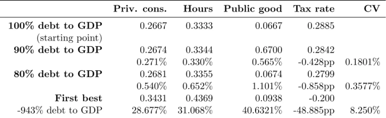
Priv. cons. Hours Public good Tax rate CV 100% debt to GDP 0.2667 0.3333 0.0667 0.2885 (starting point) 90% debt to GDP 0.2674 0.3344 0.6700 0.2842 0.271% 0.330% 0.565% -0.428pp 0.1801% 80% debt to GDP 0.2681 0.3355 0.0674 0.2799 0.540% 0.652% 1.101% -0.858pp 0.3577% First best 0.3431 0.4369 0.0938 -0.200 -943% debt to GDP 28.677% 31.068% 40.6321% -48.885pp 8.250% Table 4: Steady state comparison for different debt levels. CV is the welfare equivalent consumption variation.
5
Transition dynamics
While the previous analysis has shown potential welfare gains from lower debt levels in the long-run, this section sheds some light on the costs during the consolidation and whether an equilibrium with lower debt levels is preferable relative to the status quo if the transitional costs are taken into account. I will first present each consolidation separately, compare them and then show the importance of a maturity-structure above one period.
5.1 Fiscal consolidation
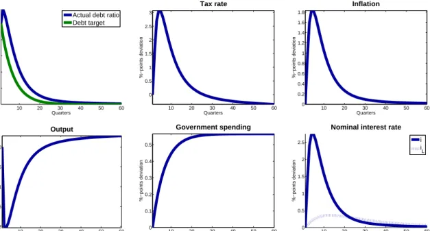
Figure 5 shows the macroeconomic effects for a tax-based consolidation. The fall in the debt target induces the labor tax rate to rise until period 6 and then to gradually convert back until its new (lower) value τnew. As a result of higher distortionary labor taxes the incentive to supply labor is reduced, leading the economy into a recession. As the previous section has shown government spending will be higher in the new long run equilibrium. Independent of how the transition will be accomplished exactly, the increase in government spending constitutes a negative wealth effect and lowers private consumption while increasing the supply of labor. This effect lowers the output drop, for instance compared to Coenen et al. (2008), to about 2%. The recession lasts for 5 to 6 years until labor supply recovers and converges to its higher long term equilibrium. As taxes reduce c.p. the after tax wage income, households bargain for higher pretax wages which increases the marginal costs for firms. Those firms that can adjust will charge higher prices which leads to inflation. The monetary authority follows the Taylor principle and raises the short term rate more than one-to-one, driving up the real short term interest rates. As can be seen from equation 4 to 3.2, and which is shown in Krause and Moyen (2013), the expected future path of the policy rate it determines the interest rate on newly issued bonds il,nt which determine the average
10 20 30 40 50 60 92 94 96 98 100 Quarters Debt to GDP in %
Actual debt ratio Debt target 10 20 30 40 50 60 0 0.5 1 1.5 2 2.5 3 Tax rate %−points deviation Quarters 10 20 30 40 50 60 0 0.2 0.4 0.6 0.8 1 1.2 1.4 1.6 1.8 Inflation %−points deviation Quarters 10 20 30 40 50 60 −2 −1.5 −1 −0.5 0 Output % deviation from ss Quarters 10 20 30 40 50 60 0 0.1 0.2 0.3 0.4 0.5 Government spending %−points deviation Quarters 10 20 30 40 50 60 0 0.5 1 1.5 2 2.5 Quarters %−points deviation
Nominal interest rate
i iL
Figure 5: Tax-based consolidation. Notes: All variables are in percentage deviation from steady state, except tax rates, inflation and interest rates which are in percentage point deviations.
payment of the portfolio ilt. As the model is solved by perfect foresight agents foresee that the policy rate will be lower in the future and thus ask for a higher interest rateil,nt but lower thanit. Since the average interest rate is a weighted sum of its previous value ilt−1 and i
l,n t
it reacts only sluggishly by a mere 0.4% compared to 2.5% of the short term interest rate. Therefore, even as the policy rate is raised according to the Taylor principle, the interest rate charged on newly issued bonds is raised less as it takes into account a smaller policy rate in the future. Additionally the increased paymentsil,nt bl,nt do not affect the budget that much as it is a relatively small fraction compared to the outstanding stock. Taking into account that inflation is higher than the nominal average long term rate the real average long term rate is reduced and therefore also the real financing needs for a given debt level.16 Additionally, the real value of nominal debt is reduced and thus dampens the financing needs to achieve the target. This mechanism will be important (and taken up again) when compared to a world with short term debt.
Figure 6 depicts the same variables for the spending-based scenario. Public good provision will be reduced up to 18% in period 6 and recovers gradually until it reaches its higher long run level gnew. The prospect of higher government expenditure coupled with lower tax rates
16After a while inflation is below the average long term rate thus increasing financing costs of the outstanding debt stock. However, as the total stock is reduced that effect is only of minor importance.
10 20 30 40 50 60 90 92 94 96 98 100 Quarters Debt to GDP in %
Actual debt ratio Debt target 10 20 30 40 50 60 −18 −16 −14 −12 −10 −8 −6 −4 −2 0 Government spending % deviation from ss Quarters 10 20 30 40 50 60 −1 −0.5 0 0.5 1 Inflation %−points deviation Quarters 10 20 30 40 50 60 −1.5 −1 −0.5 0 0.5 Output % deviation from ss Quarters 10 20 30 40 50 60 −0.4 −0.35 −0.3 −0.25 −0.2 −0.15 −0.1 −0.05 0 Output %−points deviation Quarters 10 20 30 40 50 60 −1.5 −1 −0.5 0 0.5 1 1.5 Quarters %−points deviation
Nominal interest rate
i iL
Figure 6: Spending-based consolidation. Notes: All variables are in percentage deviation from steady state, except tax rates, inflation and interest rates which are in percentage point deviations.
leads to an expansion in labor in the short run.
On the oder hand, as the government cuts spending during the transition, agents experience a positive wealth effect that increases private consumption and lowers the incentive to work. This short run positive wealth effect is more pronounced and thus drives the economy into a recession. However, compared to Coenen et al. (2008), spending reductions are associated with relatively lower recessions. The importance of future composition of variables on current dynamics is shown, for instance, by Cogan et al. (2013).17 The inflation rate rises for the first year as a result of higher production but then drops and stays below 0 before it converges slowly back to its steady state value. The cut in government spending reduces production and inflation as firms compete for private demand and thus lower prices. As households supply less labor part of the deflationary pressure is dampened. Similar to the above argument, the short term interest rate follows the inflation pattern due to the Taylor rule but the interest rates on newly issued bonds take into account the whole future path of the policy rates and thus are lowered. This reduces the average interest rate but only to a small degree as the lower rate is payed for a small fraction while the rest still pays the higher rate from steady
17In the specification of government spending transition used, there is an initial jump in output in the first period followed by a recession. The reduced long term interest rate leads to a growing demand for private consumption but public goods have not been reduced a lot in the first period. Therefore, labor supply has to increases to satisfy the demand. One can show that with a steeper decline in government spending in the first period there is always a recession so the boom depends on the specification used.
2
3
4
0
0.05
0.1
0.15
0.2
0.25
0.3
Year
Output loss relative to debt reduction
Fiscal Sacrifice Ratio
Tax hike
Spending cut
Figure 7: Fiscal sacrifice ratio ζT. Notes: The fiscal sacrifice ratio is calculated as
ζT = 1 T PT t=1Yt −Y old Y old / ¯ Bt 4Yt− ¯ Bold 4Y old .
state. In the periods with positive inflation the real average long term rate is lowered even more which eases to keep real debt close to the target. However, once inflation falls below 0, i.e. there is deflation, that first increases real average long term rates and second, also the real value of debt, thus making the adjustment process more severe. That is the reason why spending has to be cut by that large amount.
5.2 Comparing the fiscal consolidations
Both consolidation strategies lead to the same long run equilibrium, but both entailed different adjustment costs (lower government or private consumption). I use two metrics to compare the relative desirability/associated costs.
The first is the “fiscal sacrifice ratio”, a measure, that relates the output loss to the percentage point reduction of debt. For a smoother comparison I use the average output drop rather the exact drop within that period. More precisely, the ratio is defined asζT =
1 T PT t=1 Yt−Y old Y old
/Bt¯ 4Yt−
¯
Bold
4Y old
, with ¯B denoting total nominal debt. Figure 5.2 presents the ratio at a two, three and four year horizon. Within two years, both fiscal consolidations reduce the debt/GDP ratio by about 3.5% points while output falls on average about 1%, consistent with a “fiscal sacrifice ratio” of around 1/3. Increasing the time horizon reduces the sacrifice ratio as growth will catch up to its new long run level.18 Over the whole time span tax-based consolidation is associated with a lower FSR ratio than spending-based adjustments.
A second approach is to evaluate the welfare equivalent consumption variation (CV) associated with each reduction scenario, that is the permanent amount of consumption that makes the household indifferent between staying at the steady state with higher debt and moving to the lower debt steady state. It is defined as
∞
X
t=0
βt(U((1 +ν)Cold)−v(Nold) +g(Gold) = ∞
X
t=0
βt(U(Ct)−v(Nt) +g(Gt).
Positive values imply that agents want to stay at the old steady state only if they get additional permanent consumption and thus prefer the lower debt steady state. The corresponding values are -0.0639 for spending cuts and 0.0422 for tax hikes.
Therefore households are better of to consolidate only when the adjustment is tax-based. They, however, want to stay at the status quo if spending has to be adjusted. This is in line with the previous result of the FSR. A positive and higher CV for tax hikes compared to spending cuts is in contrast to Forni et al. (2010) and depends on the introduction of long term debt, as the next section will make clear.19
5.3 Comparison to one period debt
How important are the channels20 through which long term debt affect the macroeconomic implications of debt consolidation? To shed more light on this issue I will first evaluate both adjustment when only short term debt is available and then for intermediate values of maturity.
The current framework nests the one period debt model when setting γ = 1. Figures 8 and 9 depict the dynamics for the same variables as above. As one can see the transition of both fiscal consolidations is similar qualitatively, however, the magnitudes differ: Tax-based consolidation is associated with an enlarged fiscal distress. The labor tax rate roughly
18
In the first year, both sacrifice ratios are negative, however, spending cuts are preferable as output growth reduces the debt ratio while tax hikes lead to a recession with an initial increase in debt. A quantitative comparison is thus difficult.
19See, for instance, Table 8 within their paper. 20
First, strong changes in short term rates do not affect the budget position by a lot as only part of the debt is reissued and those rates depend also on future policy rates. Second, inflation/deflation affects the real financing costs and, third, the real value of nominal debt more in case of long-term debt.
10 20 30 40 50 60 92 94 96 98 100 Quarters %−points deviation Debt to GDP
Actual debt ratio Debt target 10 20 30 40 50 60 0 1 2 3 4 5 Quarters
%−points deviation from ss
Tax rate
Long term debt Short term debt
10 20 30 40 50 60 −1 −0.5 0 0.5 1 1.5 2 2.5 Quarters
%−points deviation from ss
Inflation
Long term debt Short term debt
10 20 30 40 50 60 −3.5 −3 −2.5 −2 −1.5 −1 −0.5 0 Quarters % deviation from ss Output
Long term debt Short term debt
10 20 30 40 50 60 0 0.1 0.2 0.3 0.4 0.5 Quarters % deviation from ss Government spending
Long term debt Short term debt
10 20 30 40 50 60 −1 0 1 2 3 Quarters
%−points deviation from ss
Long term interest rate
Long term debt Short term debt
Figure 8: Tax-based consolidation with short-term debt. Notes: All variables are in percent-age deviation from steady state, except tax rates, inflation and interest rates which are in percentage point deviations.
doubles to 5% points, output drops by more than 3% and the recession is more persistent. Inflation rises after an initial drop to as high as 2.5%, however, since all debt is reissued, the only surprise change in real terms is in the first period. All other price changes are already expected and priced into the interest rate. Positive inflation leads to an increase in the short term nominal and real interest rates which affects the budget more pronounced, increasing the necessary adjustment which explains the prolonged tax rise and the longer time to consolidate. In the spending-based adjustments, public goods still have to be cut by roughly 18% but recover much more quickly. As a result of the steeper drop there is deflation over the whole consolidation period. However, as the central bank cuts its policy rate that deflation results in a lower real interest rate which stimulates private demand and reduces the necessary fiscal adjustment as all of the debt is reissued and pays a lower real amount. The drop in output is more severe, however, it is not so persistent as with long-term debt. Overall, the aggregate variables do not move that much compared to the tax-based consolidation. Figure 10 illustrates the different sacrifice ratios for the model with short term debt. Spending cuts become much more preferable than tax hikes, since in the latter the output drop was much more severe. The FSR is between 2 to 5 times lower when public expenditures are adjusted and the CV is with -0.011% compared to -0.13% still negative but much lower. The difference for the results lies in the way inflation helps to mitigate fiscal consequences,
10 20 30 40 50 60 90 92 94 96 98 100 Quarters %−points deviation Debt to GDP
Actual debt ratio Debt target 10 20 30 40 50 60 −0.4 −0.35 −0.3 −0.25 −0.2 −0.15 −0.1 −0.05 0 Quarters
%−points deviation from ss
Tax rate
Long term debt Short term debt
10 20 30 40 50 60 −1 −0.5 0 0.5 1 Quarters
%−points deviation from ss
Inflation
Long term debt Short term debt
10 20 30 40 50 60 −2 −1.5 −1 −0.5 0 0.5 Quarters % deviation from ss Output
Long term debt Short term debt
10 20 30 40 50 60 −18 −16 −14 −12 −10 −8 −6 −4 −2 0 Quarters % deviation from ss Government spending
Long term debt Short term debt
10 20 30 40 50 60 −2 −1.5 −1 −0.5 0 Quarters
%−points deviation from ss
Long term interest rate
Long term debt Short term debt
Figure 9: Spending-based consolidation with short-term debt. Notes: All variables are in percentage deviation from steady state, except tax rates, inflation and interest rates which are in percentage point deviations.
First, with short term debt only, all outstanding liabilities have to be rolled over so the increase in the real financing costs directly affect the budget by a high margin. On the other hand the increase in the price level reduces the real value of debt and thus the financing costs. Overall, the effect is ambiguous ex ante. With long term debt contracts the government has to issue only part of the outstanding debt stock.21 Therefore, an increase in real rates will raise total debt servicing costs by less. Second, inflation becomes much more pronounced in reducing the real value of debt. Both effects unambiguously reduce total financing costs relative to one-period debt. This is the key mechanism why in a model with long term debt contracts, tax hikes are less disruptive than spending cuts: they are associated with higher inflation. To be quantitatively important in one period debt models inflation would need to be much larger.
To illustrate how different levels of average maturity change the result, figure 11 summarizes the sacrifice ratio and welfare equivalent consumption variation for both spending cuts and tax hikes for various maturities. In general, for higher average maturities the CV is increasing (decreasing) when consolidation is tax-(spending-)based. The FSR is decreasing for tax hikes but stays relatively constant for spending cuts across different maturities. The threshold
21
In case of a consol with γ= 0 the government only pays predetermined interest rates while the stock is rolled over. Changes in the real interest rates would thus not materialize at all.
2
3
4
0
0.5
1
1.5
2
2.5
Year
Output loss relative to debt reduction
Fiscal Sacrifice Ratio
Tax hike
Spending cut
Figure 10: Sacrifice ratio evaluated at different times for the model with short-term debt.
2 4 6 8 10 12 14 0.5 1 1.5 2 2.5
Average maturity of debt in years
Ratio
Fiscal Sacrifice Ratio for different maturities Tax hike Spending cut 2 4 6 8 10 12 14 −0.12 −0.1 −0.08 −0.06 −0.04 −0.02 0 0.02 0.04 0.06
Average maturity of debt in years
in %
Consumption variation for different maturities
Tax hike Spending cut
Figure 11: Fiscal Sacrifice Ratio and CV evaluated at different maturities for tax- and spending-based consolidation.
after which tax-based consolidation is preferable is 2 years for the CV or 4 years for the FSR. Additionally, for maturities above 3 years households prefer debt consolidation when done via higher taxes. Independent of the maturity, spending-based consolidation is never preferable.
6
Robustness
TO BE COMPLETED
Insert here robustness results with respect to parameter values, debt amount to be reduced and different time horizon to reduce given debt level. Different monetary policy accomoda-tions?
If monetary policy is fixed the results should be strengthened: Spending reductions than increase the real rate which further dampens the economy as consumption is crowded out. This will lead to a further fall in the price level. Tax-hikes will reduce the real rate and thus increase consumption which dampens the recession and increases inflation.
Higher interest rates due to higher maturity will not affect results because what is important are the relative effects not level effects.
What does change if open economy ⇒ depends on terms of trade effect of tax hikes vs. spending cuts.
Shape of CV seems to imply that proper accounting of maturity will lessen the effects. Short-term debt is very costly while the longer the average maturity the less costly tax-hikes become. However, that loss-function is concave! I.e. having 50% short-term debt and 50% 19 quarter debt, the average maturity would be 10Q and the loss will be some number. If properly account that 50%, the true loss seems to be higher.
7
Conclusion
The Great Recession has sent debt levels to a post-WWII high for several advanced economies. It seems to be a consensus that these elevated debt levels have to be reduced at some point -the question remains is when and which instruments to use. In this paper I try to shed some light on the latter and how the relative attractiveness of fiscal consolidation schemes depend on the average maturity of outstanding debt. The main difference between short and long term debt is the inflationary consequence of the fiscal consolidation and more precisely how
inflation affects real values: First, any change in the financing costs of bonds transmits only partly on the budget as just a small fraction of bonds is reissued. Second, inflation reduces the real value of debt in proportion to its average maturity. Lower real debt levels mitigate the extent to which other fiscal measures have to be raised. This inflationary impact is of minor importance in one period debt models but it is the key mechanism why in a model with long term debt contracts, tax hikes can become less disruptive than spending cuts if the average maturity is above 2 years: tax hikes are inflationary whereas spending cuts deflationary. The present analyses clarifies the important role of inflation in the consolidation process, even though raising its target rate directly might either not be desirable because of commitment inconsistencies as in Barro and Gordon (1983) or not feasible as in the case of a small country within a currency union. Therefore, when assessing the relative attractiveness of various debt reduction tools it might be important to also consider their inflationary impact.
References
Aiyagari, S. R., Marcet, A., Sargent, T. J., and Sepp¨al¨a, J. (2002). Optimal taxation without state-contingent debt. Journal of Political Economy, 110(6):1220–1254.
Aiyagari, S. R. and McGrattan, E. R. (1998). The optimum quantity of debt. Journal of Monetary Economics, 42(3):447–469.
Aizenman, J. and Marion, N. (2011). Using inflation to erode the us public debt. Journal of Macroeconomics, 33(4):524–541.
Alesina, A. and Ardagna, S. (2010). Large changes in fiscal policy: taxes versus spending. In
Tax Policy and the Economy, Volume 24, pages 35–68. The University of Chicago Press. Alesina, A., Favero, C., and Giavazzi, F. (2014). The output effect of fiscal consolidation
plans. Journal of International Economics, (0):–.
Alesina, A. and Perotti, R. (1995). Fiscal expansions and adjustments in oecd countries.
Economic policy, 10(21):205–248.
Ambler, S. (2007). The costs of inflation in new keynesian models. Bank of Canada Review, 2007(Winter):7–16.
Barro, R. J. (1979). On the determination of the public debt. The Journal of Political Economy, 87(5):940–971.
Barro, R. J. and Gordon, D. B. (1983). Rules, discretion and reputation in a model of monetary policy. Journal of monetary economics, 12(1):101–121.
Bohn, H. (2011). The economic consequences of rising us government debt: privileges at risk.
FinanzArchiv: Public Finance Analysis, 67(3):282–302.
Calvo, G. A. (1983). Staggered prices in a utility-maximizing framework.Journal of monetary Economics, 12(3):383–398.
Chatterjee, S. and Eyigungor, B. (2012). Maturity, indebtedness, and default risk. The American Economic Review, 102(6):2674–2699.
Cochrane, J. H. (1999). A frictionless view of us inflation. InNBER Macroeconomics Annual 1998, volume 13, pages 323–421. MIT Press.
Coenen, G., Mohr, M., and Straub, R. (2008). Fiscal consolidation in the euro area: Long-run benefits and short-run costs. Economic Modelling, 25(5):912–932.
Cogan, J. F., Taylor, J. B., Wieland, V., and Wolters, M. H. (2013). Fiscal consolidation strategy. Journal of Economic Dynamics and Control, 37(2):404–421.
Cole, H. L. and Kehoe, T. J. (2000). Self-fulfilling debt crises. The Review of Economic Studies, 67(1):91–116.
Conesa, J. C. and Kehoe, T. J. (2012). Gambling for redemption and self-fulfilling debt crises. Technical report, Minneapolis Fed Staff Report Nr. 465.
Dixit, A. K. and Stiglitz, J. E. (1977). Monopolistic competition and optimum product diversity. The American Economic Review, 67(3):297–308.
Eggertsson, G. B. (2011). What fiscal policy is effective at zero interest rates? In NBER Macroeconomics Annual 2010, Volume 25, pages 59–112. University of Chicago Press. Erceg, C. J. and Lind´e, J. (2013). Fiscal consolidation in a currency union: Spending cuts
vs. tax hikes. Journal of Economic Dynamics and Control, 37(2):422–445.
Faraglia, E., Marcet, A., Oikonomou, R., and Scott, A. (2013). The impact of debt levels and debt maturity on inflation. The Economic Journal, 123(566):F164–F192.
Feldstein, M. (2002). Commentary : Is there a role for discretionary fiscal policy? Proceedings - Economic Policy Symposium - Jackson Hole, pages 151–162.
Fischer, S. and Modigliani, F. (1978). Towards an understanding of the real effects and costs of inflation. Weltwirtschaftliches Archiv, 114(4):810–833.
Forni, L., Gerali, A., and Pisani, M. (2010). The macroeconomics of fiscal consolidations in euro area countries. Journal of Economic Dynamics and Control, 34(9):1791–1812.
Guajardo, J., Leigh, D., and Pescatori, A. (2014). Expansionary austerity? international evidence. Journal of the European Economic Association, 12(4):949–968.
Hall, G. J. and Sargent, T. J. (2011). Interest rate risk and other determinants of post-wwii us government debt/gdp dynamics. American Economic Journal: Macroeconomics, 3(3):192–214.
Hatchondo, J. C. and Martinez, L. (2009). Long-duration bonds and sovereign defaults.
Journal of International Economics, 79(1):117–125.
Holden, S. and Midthjell, N. (2013). Successful fiscal adjustments. does choice of fiscal in-strument matter? Does Choice of Fiscal Instrument Matter.
IMF, I. M. F. (2011). Regional economic outlook. World Economic and Financial Surveys. Jayadev, A. and Konczal, M. (2010). The boom not the slump: The right time for austerity. Krause, M. U. and Moyen, S. (2013). Public debt and changing inflation targets, volume 6.
Discussion Paper Deutsche Bundesbank.
Panizza, U. and Presbitero, A. F. (2013). Public debt and economic growth in advanced economies: A survey. Swiss Journal of Economics and Statistics, 149(2):175–204.
Reinhart, C. M., Reinhart, V. R., and Rogoff, K. S. (2012). Public debt overhangs: advanced-economy episodes since 1800. The Journal of Economic Perspectives, 26(3):69–86.
Reinhart, C. M. and Rogoff, K. S. (2010). Growth in a time of debt. American Economic Review, 100(2):573–78.
Reinhart, C. M. and Rogoff, K. S. (2013). Growth in a time of debt. Errata.
R¨ohrs, S. and Winter, C. (2014). Reducing government debt in the presence of inequality.
Unpublished Manuscript.
Roubini, N. (2011). Why Inflation Is Not a Desirable or Likely Way to Reduce Unsustainable Debts.
Sargent, T. J. and Wallace, N. (1981). Some unpleasant monetarist arithmetic. Quarterly Review, 5:1–18.
Sims, C. A. (2013). Paper money. The American Economic Review, 103(2):563–584.
Trabandt, M. and Uhlig, H. (2011). The laffer curve revisited. Journal of Monetary Eco-nomics, 58(4):305–327.
von Weizsaecker, C. C. (2011). Public debt requirements in a regime of price stability. Public Debt.
Woodford, M. (1995). Price-level determinacy without control of a monetary aggregate.
Carnegie-Rochester Conference Series on Public Policy, 43(1):1–46.
Woodford, M. (2001). Fiscal requirements for price stability. Journal of Money, Credit and Banking, 33(3):669–728.