Current Density Impedance Imaging with Complete Electrode Model

Current Density Impedance Imaging with

Complete Electrode Model

Alexandru Tamasan

jointly with A. Nachman & J. Veras

University of Central Florida Work supported by NSF

Outline

In motivation

Hybrid methods in Inverse Problems Current density based EIT

Acquiring the interior data

The forward problem

The Complete Electrode Model

The Inverse Problem

Characterization of non-uniqueness Phase retrieval

Restoring uniqueness

A numerical algorithm and experiment Conclusions

Coupled Physics Imaging Methods

Combine high contrast & high resolution

I Elastography: elastic waves & ultrasound/MRI⇒stiffness

I Thermo/PhotoAcoustic: UV light & sound⇒embedded acoustic sources

I AcoustoOptics: light & sound⇒absorption and scattering

I Coupled Physics Electrical Impedance Tomography

I _{Current density impedance imagingCDII: Joy& Nachman} since 2002, Seo et al. 2002

I _{MREIT (Bz-methods): Seo et al. since 2003}

I _{Ultrasound modulated EIT: Capdebosq et at. 2008, Bal et} al. 2009

I Impedance acoustic: Scherzer et al. 2009

I Lorentz force driven EIT: Ammari et al. since 2013 I ...

Current density tracing inside an object

Magnetic resonance data:

M

: Ω

→

_C

Aquiring the interior data

One MR scan⇒longitudinal componentBz (along gantry) of

the magnetic fieldB= (Bx,By,Bz)

Bz(x,y,z0) = 1 2γT Imlog M+(x,y,z0) M−(x,y,z0)

I MREIT (Seo at al. since 2003): DoesBz uniquely

determine the electrical conductivity? In general, not known.

I CDII (Nachman et al since 2002, Seo (2002)) : + two rotation of the object

⇒B⇒J= 1

µ0 ∇ ×B I Anisotropic case: Bal & Monard (2013), unique

determination Hoell-Moradifam-Nachman (2014, within conformal class)

Outline

In motivation

Hybrid methods in Inverse Problems Current density based EIT

Acquiring the interior data

The forward problem

The Complete Electrode Model

The Inverse Problem

Characterization of non-uniqueness Phase retrieval

Restoring uniqueness

A numerical algorithm and experiment Conclusions

Complete Electrode Model

(Somersalo-Cheney-Isaacson ’92)

Ω⊂Rnbounded with Lipschitz boundary∂Ω,

N+1 electrodes:e_k ⊂∂Ω,k =0, ...,N, ≤_Re{σ} ≤1/, ≤Re{zk} ≤1/,k =0,1, ...,N, ∇ ·σ∇u=0, inΩ, u+zkσ ∂u ∂ν ≡const =Uk onek, fork =0, ...,N, Z ek σ∂u ∂νds=Ik, fork =0, ...,N, ∂u ∂ν =0, on∂Ω\ N [ k=0 ek,

Forward problem (CEM) is well posed

Based on Lax-Milgram lemma:

Theorem(Somersalo- Cheney- Isaacson ’92) Provided

N

X

k=0

Ik =0,

there is a unique solutionhu(x),(U0, ....,UN)i ∈H1(Ω)×CN+1

Normalization

Uniqueness up to a constant: hu(x) +c,(U0+c, ....,UN+c)ialso a solution. ∇ ·σ∇(u+c) =0, inΩ, (u+c) +zkσ ∂(u+c) ∂ν ≡const =Uk +c onek, fork =0, ...,N, Z ek σ∂(u+c) ∂ν ds =Ik, fork =0, ...,N, ∂(u+c) ∂ν =0, on∂Ω\ N [ k=0 ek,

Normalization:fix a constant by seekingU= (U0, ...,UN)with

PN

New properties in the real valued case

σ(x),z0(x), ...,zN(x)∈R U∈Π :={(U0, ...UN)∈RN+1: N X k=0 U_k =0}

I Maximum Principle for CEM: The maximum and minimum of the voltage potentialuoccur on the electrodes.

I A Poicar ´e Inequality (not necessarily connected with CEM):∃C >0 dependent only onΩandek ⊂∂Ωsuch that ∀u ∈H1(Ω)and∀U= (U0, ...,UN)∈Π : Z Ω u2+ N X k=0 U_k2≤C Z Ω |∇u|2dx + N X k=0 Z ek (u−Uk)2ds !

The Dirichlet principle for the CEM

Consider the functional

Fσ(u,U) := 1 2 Z ∂Ω σ|∇u|2dx +1 2 N X k=0 Z ek 1 zk (u−Uk)2ds− N X k=0 IkUk.

RecallΩ,Π,ek ⊂∂Ω,zk, fork =0, ...,N,σ, and

N X k=0 Ik =0 (?) Theorem(Nachman-T-Veras ’14) (i) Independently of(?): ∃! (u,U) =argmin_H1_(Ω)×ΠFσ (ii) If(?)holds:

Formulation of an Inverse Problem

Given:Ω,ek ⊂∂Ωwithzk >0, andI1, ....,IN,

(thenI0:=−PNk=1Ik),

and|J|=σ|∇u|insideΩ,

Formulation of an Inverse Problem

Given:Ω,ek ⊂∂Ωwithzk >0, andIk,k=1, ...,N (then

I0:=−PNk=1Ik), and|J|=σ|∇u|inside, Findσ.

Not possible: Ω = (0,1)×(0,1),

Top side:e1withz1>0, injectI1=1

Bottom side:e0withz0=z1+1, extractI0=−1

Measure the magnitude|J| ≡1 inside.

Arbitraryϕ: [0,1]→[ϕ(0), ϕ(1)]increasing, Lipschitz with

ϕ(0) +ϕ(1) =1.

Then:uϕ(x,y) :=ϕ(y)voltage forσϕ(x,y) =1/ϕ0(y). Yet for all suchϕ,

Generic non-uniqueness

Let(u,U)∈H1(Ω)×Πbe the solution of CEM for someσ.

ϕ∈Lip(u(Ω))be an increasing function of one variable,

ϕ(t) =t+ck whenevert ∈u(ek), for eachk =0, ...,N, and

constantsck satisfying

PN

k=0ck =0. Then

uϕ :=ϕ◦u (1)

is a voltage potential for CEM with

σϕ :=

σ

ϕ0◦u, (2)

and has the same interior data

Characterization of Non-uniqueness

Theorem(Nachman-T-Veras ’14) Recall assumptions on

Ω⊂_Rd _{be bounded, connectedC}1,α_,e

k ⊂∂Ω,zk >0,Ik,

k =0, ...,N.

Let(u,U),(v,V)∈H1(Ω)×Π, be the CEM solutions for unknown conductivitiesσ,σ˜ ∈Cα(Ω)with

|J|:=σ|∇u|= ˜σ|∇v|>0a.e.inΩ.

Then∃ϕ∈C1(u(Ω)), withϕ0(t)>0 a.e. inΩ, such that

v =ϕ◦u, inΩ,

˜

σ = σ

ϕ0◦u, a.e. inΩ.

Moreover, for eachk =0, ...,N andt∈v(ek),

Idea: reduction to a minimization problem

Inverse hybrid problem: Consider

G|J|(v,V) = Z Ω |J| |∇v|dx+1 2 N X k=0 Z ek 1 z_k(v−Vk) 2_ds− N X k=0 IkVk,

I solutions of CEM are global minimizers ofG|J|over

H1(Ω)×Π.

I Geometry of the equipotential sets are uniquely determined! Contrast with Dirichlet

Contrast with functional in the forward model

Fσ(v,V) := 1 2 Z ∂Ω σ|∇v|2dx+1 2 N X k=0 Z ek 1 zk (v−Vk)2ds− N X k=0 IkVk.

Corollaries

I Phase retrieval(Nachman-T-Veras’14) Same hypotheses (recall).

|J|=|˜J| ⇒J= ˜J.

I There is uniqueness (and a reconstruction method) from the magnitudes oftwocurrents via a local formula (Nachman et al., Lee 2004)

I TheJ-substitution algorithm via magnitudes oftwo

Knowledge of the potential on a boundary curve

joining the electrodes restores uniqueness

Theorem(Nachman-T-Veras ’14) In addition to the hypotheses of the characterization theorem if

u|_Γ= ˜u|_Γ+C,

for someC, andΓa curve joining the electrodes, then

u= ˜u+C inΩ, σ= ˜σinΩ.

A minimization algorithm for

G

G|J|(v,V) = Z Ω |J| |∇v|dx+ N X k=0 Z ek 1 2zk (v −Vk)2ds− N X k=0 IkVk,

LemmaAssume thatv ∈H1(Ω)satisfies

≤ a

|∇v|≤

1

,

for some >0, and let(u,U)∈H1(Ω)×Πbe the unique solution for CEM withσ :=a/|∇v|. Then

Ga(u,U)≤Ga(v,V), for allV ∈Π.

A minimization algorithm

I Withσngiven: Solve CEM for the unique solution(un,Un); I If essinfk∇un− ∇un−1k> δ essinf|J|, update σn+1:=min max |J| |∇un| , ,1 and repeat; I else STOP.

Enough for the phase retrieval:

J≈ |J| ∇un |∇un|

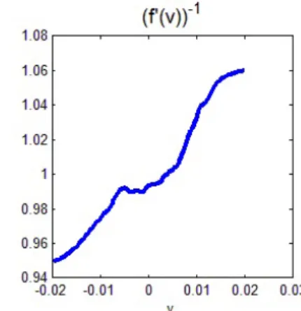
Using the voltage on

Γ

Letnbe the last iteration and set

σn+1:= |J| ∇un

.

The Characterization Theorem

⇒u(x)≈f(un(x)).

Read off the measured data onΓto determine the scaling functionf :u(Γ)→un(Γ). Then σ(x)≈ 1 f0_(u n(x)) σn+1(x).

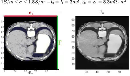
Reconstruction results in a numerical experiment

1S/m≤σ ≤1.8S/m,−I0=I1=3mA,z0=z1=8.3mΩ·m2

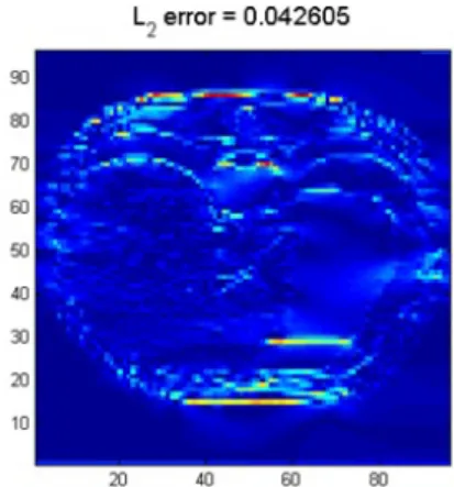
Voltage potential scaling along

Γ

Figure :L2_{-Error: Understood from the stability in the linearized case}

Some learnings

I in the more realistic CEM. the magnitude of one current density by itself cannot determine an isotropic conductivity

I the magnitude of two currents uniquely determine the conductivity (up to an additive constant)

I in the isotropic case: the phase of the current is uniquely determined from its magnitude (not known in the

anisotropic case)

I knowledge of the voltage potential along a curve restores uniqueness

I the method is constructive